
A Physics-Guided Deep Learning Model for 10-h Dead Fuel Moisture Content Estimation


Abstract
:1. Introduction
2. Materials
3. Methods
3.1. Physics-Guide Model
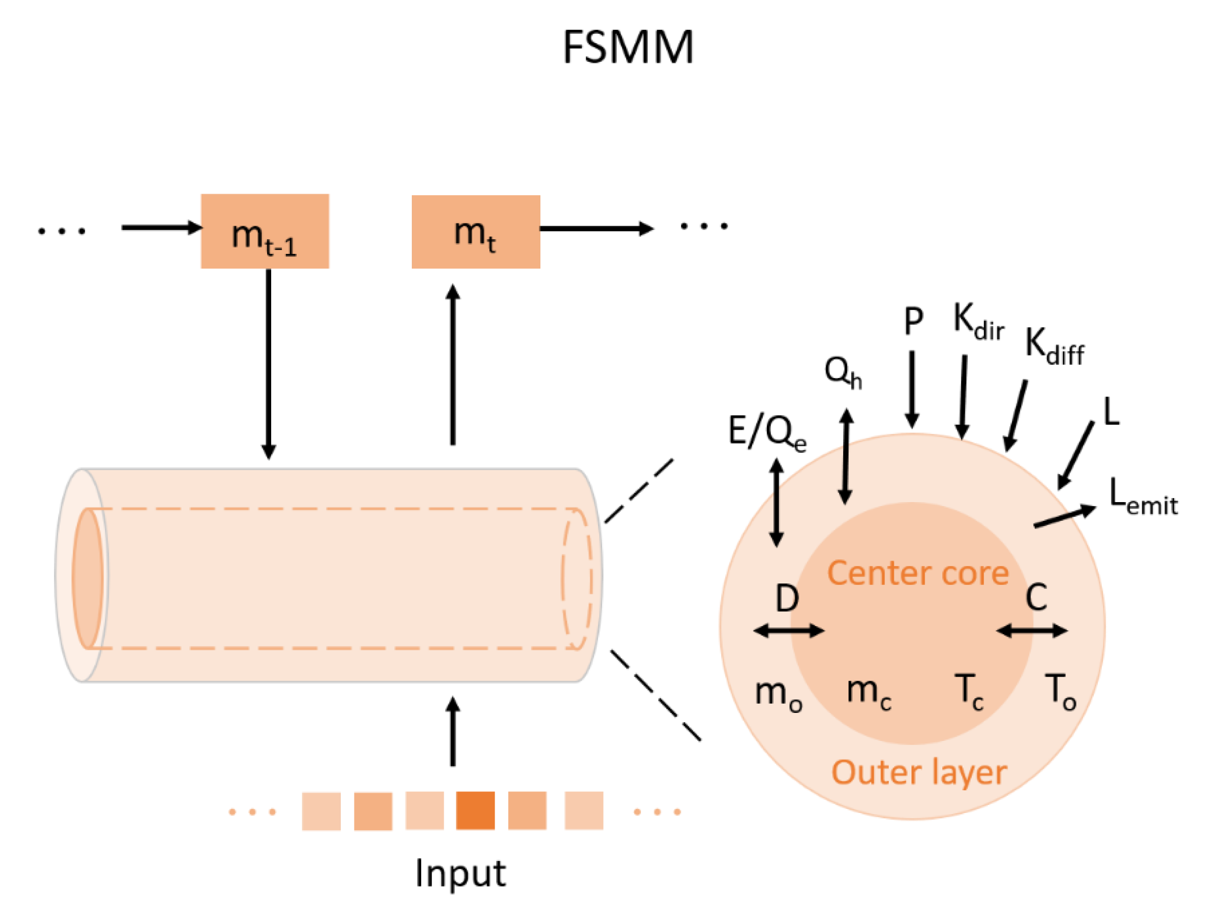
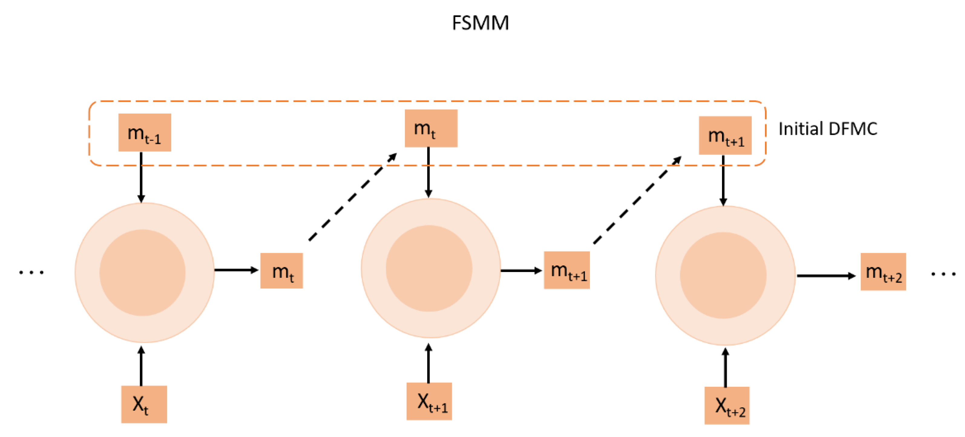
3.1.1. FSMM Model
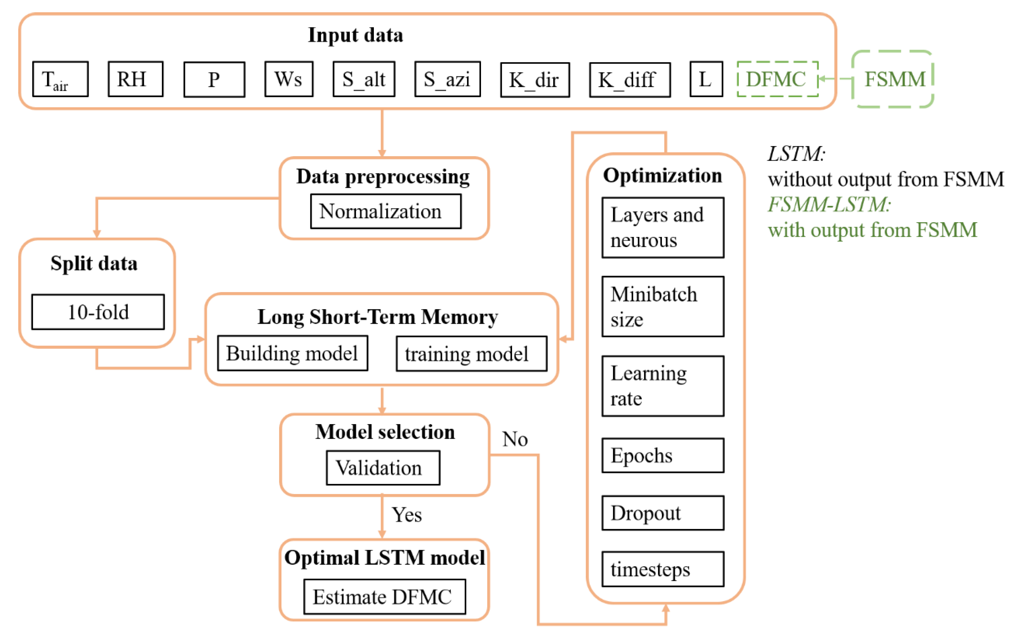
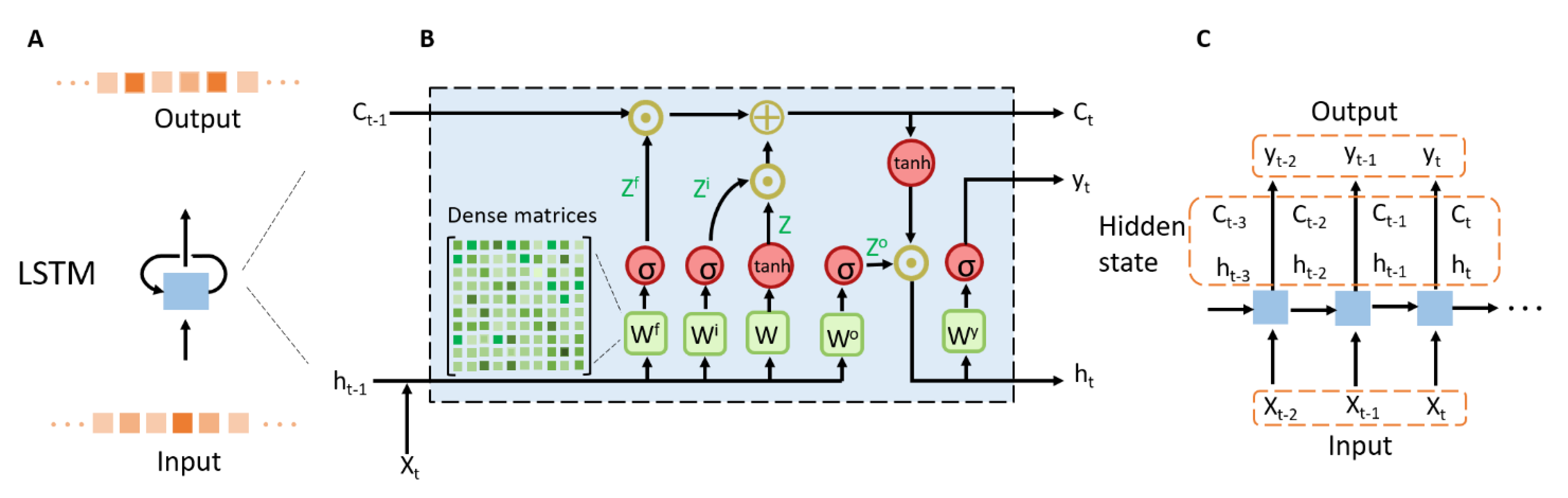
3.1.2. LSTM Network
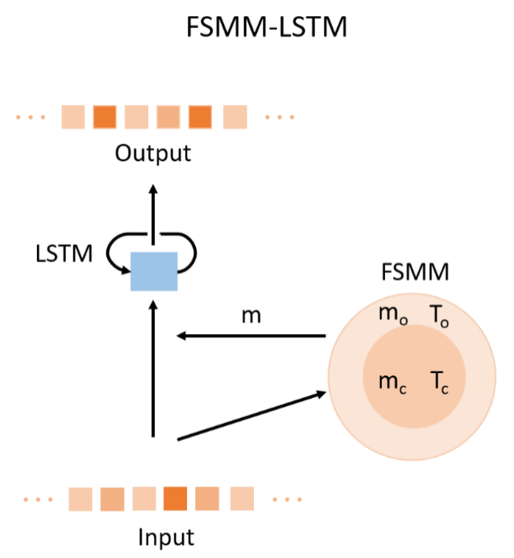
3.1.3. FSMM-LSTM Network
3.2. Model Comparison
3.2.1. MLR
3.2.2. Random Forest
3.2.3. ANN
3.3. Model Evaluation
4. Results
5. Discussion
6. Conclusions
Author Contributions
Funding
Data Availability Statement
Acknowledgments
Conflicts of Interest
References
- Sullivan, A.L. Wildland surface fire spread modelling, 1990–2007. 2: Empirical and quasi-empirical models. Int. J. Wildland Fire 2009, 18, 369–386. [Google Scholar] [CrossRef] [Green Version]
- Shakesby, R.A.; Doerr, S.H. Wildfire as a hydrological and geomorphological agent. Earth Sci. Rev. 2006, 74, 269–307. [Google Scholar] [CrossRef]
- Van Der Werf, G.R.; Randerson, J.T.; Giglio, L.; Van Leeuwen, T.T.; Chen, Y.; Rogers, B.M.; Mu, M.; Van Marle, M.J.E.; Morton, D.C.; Collatz, G.J.; et al. Global fire emissions estimates during 1997–2016. Earth Syst. Sci. Data 2017, 9, 697–720. [Google Scholar] [CrossRef] [Green Version]
- Wei, X.; Hayes, D.J.; Fraver, S.; Chen, G. Global pyrogenic carbon production during recent decades has created the potential for a large, long-term sink of atmospheric CO. J. Geophys. Res. Biogeosci. 2018, 123, 3682–3696. [Google Scholar] [CrossRef]
- Randerson, J.T.; Liu, H.; Flanner, M.; Chambers, S.; Jin, Y.; Hess, P.G.; Pfister, G.; Mack, M.C.; Treseder, K.; Welp, L.; et al. The Impact of Boreal Forest Fire on Climate Warming. Science 2006, 314, 1130–1132. [Google Scholar] [CrossRef] [PubMed] [Green Version]
- Crutzen, P.J.; Andreae, M.O. Biomass burning in the tropics: Impact on atmospheric chemistry and biogeochemical cycles. Science 1990, 250, 1669–1678. [Google Scholar] [CrossRef] [PubMed]
- Lelieveld, J.; Evans, J.S.; Fnais, M.; Giannadaki, D.; Pozzer, A. The contribution of outdoor air pollution sources to premature mortality on a global scale. Nature 2015, 525, 367–371. [Google Scholar] [CrossRef]
- Moritz, M.A.; Batllori, E.; Bradstock, R.A.; Gill, A.M.; Handmer, J.; Hessburg, P.F.; Leonard, J.; McCaffrey, S.; Odion, D.C.; Schoennagel, T.; et al. Learning to coexist with wildfire. Nature 2014, 515, 58–66. [Google Scholar] [CrossRef]
- Rao, K.; Williams, A.P.; Flefil, J.F.; Konings, A.G. SAR-enhanced mapping of live fuel moisture content. Remote Sens. Environ. 2020, 245, 111797. [Google Scholar] [CrossRef]
- Quan, X.; Yebra, M.; Riaño, D.; He, B.; Lai, G.; Liu, X. Global fuel moisture content mapping from MODIS. Int. J. Appl. Earth Obs. Geoinf. 2021, 101, 102354. [Google Scholar] [CrossRef]
- Wang, L.; Quan, X.; He, B.; Yebra, M.; Xing, M.; Liu, X. Assessment of the dual polarimetric sentinel-1A data for forest fuel moisture content estimation. Remote Sens. 2019, 11, 1568. [Google Scholar] [CrossRef] [Green Version]
- Yebra, M.; Scortechini, G.; Badi, A.; Beget, M.E.; Boer, M.M.; Bradstock, R.; Chuvieco, E.; Danson, F.M.; Dennison, P.; De Dios, V.R.; et al. Globe-LFMC, a global plant water status database for vegetation ecophysiology and wildfire applications. Sci. Data 2019, 6, 1–8. [Google Scholar]
- Quan, X.; He, B.; Yebra, M.; Liu, X.; Liu, X.; Zhung, X.; Cao, H. Retrieval of Fuel Moisture Content from Himawari-8 Product: Towards Real-Time Wildfire Risk Assessment. In Proceedings of the 2018 IEEE International Geoscience & Remote Sensing Symposium (IGARSS), Valencia, Spain, 22–27 July 2018; pp. 7660–7663. [Google Scholar]
- Rothermel, R.C. How to Predict the Spread and Intensity of Forest and Range Fires; US Department of Agriculture, Forest Service, Intermountain Forest and Range Experiment Station: Ogden, UT, USA, 1983; Volume 143. [Google Scholar]
- Viney, N.R. A review of fine fuel moisture modelling. Int. J. Wildland Fire 1991, 1, 215–234. [Google Scholar] [CrossRef]
- Matthews, S. Dead fuel moisture research: 1991. Int. J. Wildland Fire 2014, 23, 78–92. [Google Scholar] [CrossRef] [Green Version]
- Nolan, R.H.; de Dios, V.R.; Boer, M.M.; Caccamo, G.; Goulden, M.L.; Bradstock, R.A. Predicting dead fine fuel moisture at regional scales using vapour pressure deficit from MODIS and gridded weather data. Remote Sens. Environ. 2016, 174, 100–108. [Google Scholar] [CrossRef] [Green Version]
- Catchpole, E.; Catchpole, W.; Viney, N.; McCaw, W.; Marsden-Smedley, J. Estimating fuel response time and predicting fuel moisture content from field data. Int. J. Wildland Fire 2001, 10, 215–222. [Google Scholar] [CrossRef] [Green Version]
- Nieto, H.; Aguado, I.; Chuvieco, E.; Sandholt, I. Dead fuel moisture estimation with MSG–SEVIRI data. Retrieval of meteorological data for the calculation of the equilibrium moisture content. Agric. For. Meteorol. 2010, 150, 861–870. [Google Scholar] [CrossRef] [Green Version]
- Walding, N.G.; Williams, H.T.; McGarvie, S.; Belcher, C.M. A comparison of the US National Fire Danger Rating System (NFDRS) with recorded fire occurrence and final fire size. Int. J. Wildland Fire 2018, 27, 99–113. [Google Scholar] [CrossRef]
- Bradshaw, L.S. The 1978 National Fire-Danger Rating System: Technical Documentation; US Department of Agriculture, Forest Service, Intermountain Forest and Range Experiment Station: Ogden, UT, USA, 1984. [Google Scholar] [CrossRef]
- Matthews, S. A process-based model of fine fuel moisture. Int. J. Wildland Fire 2006, 15, 155–168. [Google Scholar] [CrossRef]
- Matthews, S.; Gould, J.; McCaw, L. Simple models for predicting dead fuel moisture in eucalyptus forests. Int. J. Wildland Fire 2010, 19, 459–467. [Google Scholar] [CrossRef]
- de Dios, V.R.; Fellows, A.W.; Nolan, R.H.; Boer, M.M.; Bradstock, R.A.; Domingo, F.; Goulden, M.L. A semi-mechanistic model for predicting the moisture content of fine litter. Agric. For. Meteorol. 2015, 203, 64–73. [Google Scholar] [CrossRef] [Green Version]
- Lee, H.; Won, M.; Yoon, S.; Jang, K. Estimation of 10-Hour Fuel Moisture Content Using Meteorological Data: A Model Inter-Comparison Study. Forests 2020, 11, 982. [Google Scholar] [CrossRef]
- Sharples, J.; McRae, R.; Weber, R.; Gill, A.M. A simple index for assessing fuel moisture content. Environ. Model. Softw. 2009, 24, 637–646. [Google Scholar] [CrossRef]
- Alves, M.; Batista, A.; Soares, R.; Ottaviano, M.; Marchetti, M. Fuel moisture sampling and modeling in Pinus elliottii Engelm. plantations based on weather conditions in Paraná-Brazil. iFor. Biogeosci. For. 2009, 2, 99. [Google Scholar] [CrossRef] [Green Version]
- Anderson, H.E. Moisture diffusivity and response time in fine forest fuels. Can. J. For. Res. 1990, 20, 315–325. [Google Scholar] [CrossRef]
- Simard, A. The Moisture Content of Forest Fuels–I. A Review of the Basic Concepts; Information Report FF-X-14; Canadian Department of Forest and Rural Development, Forest Fire Research Institute: Ottawa, ON, Canada, 1968. [Google Scholar]
- Van Wagner, C. Equilibrium Moisture Contents of Some Fine Forest Fuels in Eastern Canada; Information Report PS-X-36; Canadian Forestry Service, Petawawa Forest Experiment Station: Chalk River, ON, Canada, 1972. [Google Scholar]
- Van Wagner, C.E. Development and Structure of the Canadian Forest Fire Weather Index System; Forestry Technical Report 35; Canadian Forest Service, Petawawa National Forestry Institute: Chalk River, ON, Canada, 1987. [Google Scholar]
- Bilgili, E.; Coskuner, K.A.; Usta, Y.; Saglam, B.; Kucuk, O.; Berber, T.; Goltas, M. Diurnal surface fuel moisture prediction model for Calabrian pine stands in Turkey. iFor. Biogeosci. For. 2019, 12, 262. [Google Scholar] [CrossRef]
- Venäläinen, A.; Heikinheimo, M. Meteorological data for agricultural applications. Phys. Chem. Earth 2002, 27, 1045–1050. [Google Scholar] [CrossRef]
- Tamai, K. Estimation of model for litter moisture content ratio on forest floor. In Soil-Vegetation-Atmosphere Transfer Schemes and Large-Scale Hydrological Models: Proceedings of an International Symposium (Symposium S5) Held During the Sixth Scientific Assembly of the International Association of Hydrological Sciences (IAHS), Maastricht, The Netherlands, 18–27 July 2001; Volume 270, pp. 53–58.
- Byram, G.; Nelson, R. An Analysis of the Drying Process in Forest Fuel Material; US Department of Agriculture Forest Service, Southern Research Station: Asheville, NC, USA, 2015; Volume 200, pp. 1–45. [Google Scholar]
- Nelson, R.M., Jr. A method for describing equilibrium moisture content of forest fuels. Can. J. For. Res. 1984, 14, 597–600. [Google Scholar] [CrossRef]
- Tanskanen, H.; Venäläinen, A. The relationship between fire activity and fire weather indices at different stages of the growing season in Finland. Boreal Environ. Res. 2008, 13, 285–302. [Google Scholar]
- Nelson, R.M., Jr. Prediction of diurnal change in 10-h fuel stick moisture content. Can. J. For. Res. 2000, 30, 1071–1087. [Google Scholar] [CrossRef]
- Quan, X.; Li, Y.; He, B.; Cary, G.; Lai, G. Application of Landsat ETM+ and OLI Data for Foliage Fuel Load Monitoring Using Radiative Transfer Model and Machine Learning Method. IEEE J. Sel. Top. Appl. Earth Obs. Remote Sens. 2021, 14, 5100–5110. [Google Scholar] [CrossRef]
- Wolanin, A.; Camps-Valls, G.; Gómez-Chova, L.; Mateo-García, G.; Guanter, L. Estimating Crop Primary Productivity with Sentinel-2 and Landsat 8 using Machine Learning Methods Trained with Radiative Transfer Simulations. Remote Sens. Environ. 2019, 225, 441–457. [Google Scholar] [CrossRef]
- Mishra, S.; Molinaro, R. Physics Informed Neural Networks for Simulating Radiative Transfer. J. Quant. Spectrosc. Radiat. Transf. 2020, 270, 107705. [Google Scholar] [CrossRef]
- Karpatne, A.; Watkins, W.; Read, J.; Kumar, V. Physics-guided Neural Networks (PGNN): An Application in Lake Temperature Modeling. arXiv 2017, arXiv:1710.11431. Available online: https://arxiv.org/pdf/1710.11431.pdf (accessed on 15 May 2021).
- Daw, A.; Thomas, R.Q.; Carey, C.C.; Read, J.S.; Appling, A.P.; Karpatne, A. Physics-Guided Architecture (PGA) of Neural Networks for Quantifying Uncertainty in Lake Temperature Modeling. In Proceedings of the 2020 SIAM International Conference on Data Mining, Society for Industrial & Applied Mathematics (SIAM), Cincinnati, OH, USA, 7–9 May 2020; pp. 532–540. [Google Scholar]
- Bolderman, M.; Lazar, M.; Butler, H. Physics-Guided Neural Networks for Inversion-based Feedforward Control applied to Linear Motors. arXiv 2021, arXiv:2103.060922021. [Google Scholar]
- Greff, K.; Srivastava, R.K.; Koutnik, J.; Steunebrink, B.R.; Schmidhuber, J. LSTM: A Search Space Odyssey. IEEE Trans. Neural Netw. Learn. Syst. 2017, 28, 2222–2232. [Google Scholar] [CrossRef] [Green Version]
- Zhanga, J.; Yan, Z.; Zhanga, X.; Ming, Y.; Yangb, J. Developing a Long Short-Term Memory (LSTM) based model for predicting water table depth in agricultural areas. J. Hydrol. 2018, 561, 918–929. [Google Scholar] [CrossRef]
- Ata, A.A.; Tiantian, Y.; Hsu, K.; Sorooshian, S.; Lin, J.; Peng, Q. Short-Term Precipitation Forecast Based on the PERSIANN System and LSTM Recurrent Neural Networks. J. Geophys. Res. Atmos. 2018, 123, 12543–12563. [Google Scholar]
- Hosman, T.; Vilela, M.; Milstein, D.; Kelemen, J.N.; Brandman, D.M.; Hochberg, L.R.; Simeral, J.D. BCI decoder performance comparison of an LSTM recurrent neural network and a Kalman filter in retrospective simulation. In Proceedings of the 2019 9th International IEEE/EMBS Conference on Neural Engineering (NER), San Francisco, CA, USA, 20–23 March 2019; pp. 1066–1071. [Google Scholar]
- Van, D.; Moore, R.D.; Mckendry, I.G. A model for simulating the moisture content of standardized fuel sticks of various sizes. Agric. For. Meteorol. 2017, 236, 123–134. [Google Scholar]
- Tamai, K.; Goto, Y. The Estimation Of Temporal And Spatial Fluctuations In A Forest Fire Hazard Index–The Case Of A Forested Public Area In Japan. WIT Trans. Ecol. Environ. 2008, 119, 397–404. [Google Scholar]
- Carlson, J.D.; Bradshaw, L.S.; Nelson, R.M.; Bensch, R.R.; Jabrzemski, R. Application of the Nelson model to four timelag fuel classes using Oklahoma field observations: Model evaluation and comparison with National Fire Danger Rating System algorithms. Int. J. Wildland Fire 2007, 16, 204–216. [Google Scholar] [CrossRef]
- Sahin, S.O.; Kozat, S.S. Nonuniformly Sampled Data Processing Using LSTM Networks. EEE Trans. Neural Netw. Learn. Syst. 2018, 30, 1452–1461. [Google Scholar]
- Yuan, X.; Li, L.; Wang, Y. Nonlinear Dynamic Soft Sensor Modeling with Supervised Long Short-Term Memory Network. IEEE Trans. Ind. Inform. 2020, 16, 3168–3176. [Google Scholar] [CrossRef]
- Ketkar, N. Introduction to Keras. In Deep Learning with Python; Springer: Berlin/Heidelberg, Germany, 2017; pp. 97–111. [Google Scholar]
- Abadi, M.; Barham, P.; Chen, J.; Chen, Z.; Davis, A.; Dean, J.; Devin, M.; Ghemawat, S.; Irving, G.; Isard, M.; et al. TensorFlow: A system for large-scale machine learning. In Proceedings of the 12th USENIX Symposium on Operating Systems Design and Implementation (OSDI 16), Savannah, GA, USA, 2–4 November 2016; pp. 265–283. [Google Scholar]
- Liu, H.; Zhou, Q.; Zhang, S.; Deng, X. Estimation of Summer Air Temperature over China Using Himawari-8 AHI and Numerical Weather Prediction Data. Adv. Meteorol. 2019, 2019, 2385310. [Google Scholar] [CrossRef] [Green Version]
- Ahmad, M.W.; Mourshed, M.; Rezgui, Y. Trees vs. Neurons: Comparison between random forest and ANN for high-resolution prediction of building energy consumption. Energy Build. 2017, 147, 77–89. [Google Scholar] [CrossRef]
- Tranmer, M.; Elliot, M. Multiple Linear Regression; Cathie Marsh Centre for Census and Survey Research: Manchester, UK, 2008. [Google Scholar]
- Breiman, L. Random forests. Mach. Learn. 2001, 45, 5–32. [Google Scholar] [CrossRef] [Green Version]
- James, G.; Witten, D.; Hastie, T.; Tibshirani, R. An Introduction to Statistical Learning; Springer: New York, NY, USA, 2013; Volume 103. [Google Scholar]
- Liaw, A.; Wiener, M. Classification and regression by randomForest. R News 2002, 2, 18–22. [Google Scholar]
- Jenkins, B.; Tanguay, A. Handbook of Neural Computing and Neural Networks; MIT Press: Boston, MA, USA, 1995. [Google Scholar]
- Bulsari, A. Some analytical solutions to the general approximation problem for feedforward neural networks. Neural Netw. 1993, 6, 991–996. [Google Scholar] [CrossRef]
- Wu, Y.-C.; Feng, J.-W. Development and application of artificial neural network. Wirel. Pers. Commun. 2018, 102, 1645–1656. [Google Scholar] [CrossRef]
- Gui, T.; Zhang, Q.; Zhao, L.; Lin, Y.; Peng, M.; Gong, J.; Huang, X. Long short-term memory with dynamic skip connections. Proc. AAAI Conf. Artif. Intell. 2019, 33, 6481–6488. [Google Scholar] [CrossRef]
- Aguado, I.; Chuvieco, E.; Borén, R.; Nieto, H. Estimation of dead fuel moisture content from meteorological data in Mediterranean areas. Applications in fire danger assessment. Int. J. Wildland Fire 2007, 16, 390–397. [Google Scholar] [CrossRef]


| Number | Input Drives | Abbreviation |
|---|---|---|
| 1 | Air temperature (°C) | Tair |
| 2 | Relative humidity (0–100%) | RH |
| 3 | Rainfall (cm) | P |
| 4 | Wind speed (m/s) | Ws |
| 5 | Sun altitude (rad) | Salt |
| 6 | Sun azimuth (rad) | Sazi |
| 7 | Downwelling direct shortwave radiation (W/m2) | Kdir |
| 8 | Downwelling diffuse shortwave radiation (W/m2) | Kdiff |
| 9 | Downwelling longwave radiation (W/m2) | L |
| Model | Parameter | Value | Parameter | Value |
|---|---|---|---|---|
| LSTM | Hidden units | 45 | Dropout | 0.7 |
| Batch size | 4 | Timestep | 20 | |
| Learning rate | 510(−3) | Patience | 65 | |
| Optimizer | Adam | Loss | Mean square error | |
| FSMM-LSTM | Hidden units | 65 | Dropout | 0.1 |
| Batch size | 16 | Timestep | 20 | |
| Learning rate | 110(−3) | Patience | 50 | |
| Optimizer | Adam | Loss | Mean square error |
| Model | MAE (%) | RMSE (%) | R2 | Calibration Time | Test Time |
|---|---|---|---|---|---|
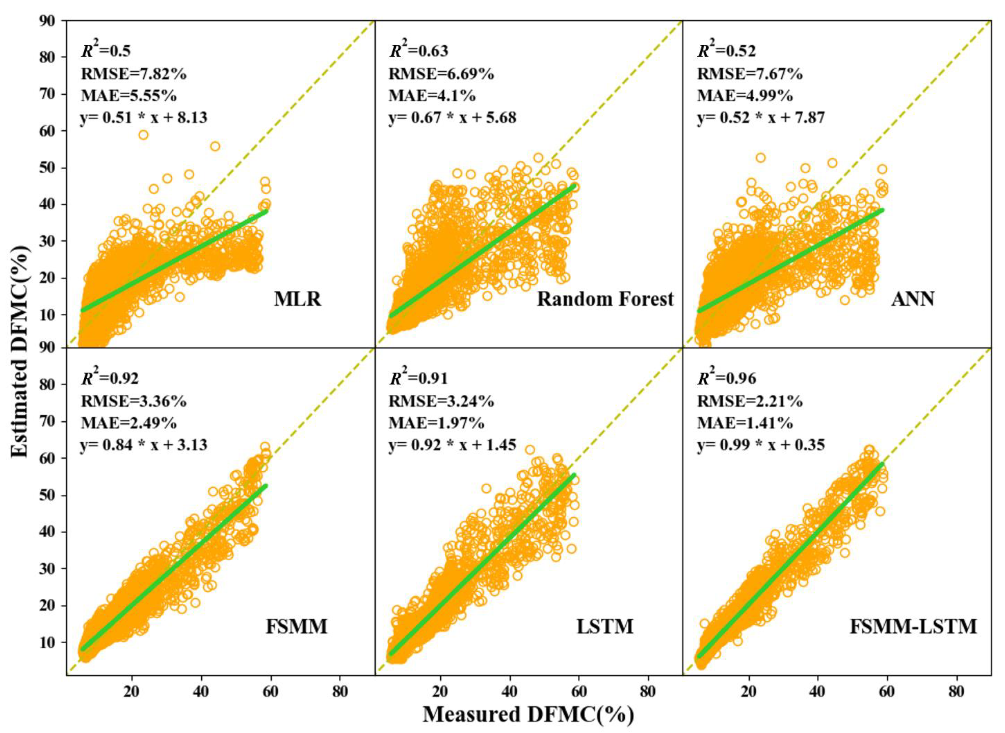
| MLR | 5.55 | 7.82 | 0.5 | <2 (second) | <1 (second) |
| Random Forest | 4.1 | 6.69 | 0.63 | <4 (second) | <1 (second) |
| ANN | 4.99 | 7.67 | 0.52 | <4 (second) | <1 (second) |
| FSMM | 2.49 | 3.36 | 0.92 | 53.75 (hour) | 7.53 (hour) |
| LSTM | 1.97 | 3.24 | 0.91 | <2 (minute) | <2 (second) |
| FSMM-LSTM | 1.41 | 2.21 | 0.96 | 60.31 (hour) | <2 (second) |
Publisher’s Note: MDPI stays neutral with regard to jurisdictional claims in published maps and institutional affiliations. |
© 2021 by the authors. Licensee MDPI, Basel, Switzerland. This article is an open access article distributed under the terms and conditions of the Creative Commons Attribution (CC BY) license (https://creativecommons.org/licenses/by/4.0/).
Share and Cite
Fan, C.; He, B. A Physics-Guided Deep Learning Model for 10-h Dead Fuel Moisture Content Estimation. Forests 2021, 12, 933. https://doi.org/10.3390/f12070933
Fan C, He B. A Physics-Guided Deep Learning Model for 10-h Dead Fuel Moisture Content Estimation. Forests. 2021; 12(7):933. https://doi.org/10.3390/f12070933
Chicago/Turabian StyleFan, Chunquan, and Binbin He. 2021. "A Physics-Guided Deep Learning Model for 10-h Dead Fuel Moisture Content Estimation" Forests 12, no. 7: 933. https://doi.org/10.3390/f12070933
APA StyleFan, C., & He, B. (2021). A Physics-Guided Deep Learning Model for 10-h Dead Fuel Moisture Content Estimation. Forests, 12(7), 933. https://doi.org/10.3390/f12070933