Abstract
Natural forests serve as the main component of the forest ecosystem. An in-depth interpretation of tree composition and structure of forest community is of great significance for natural forest conservation, monitoring, management, and near-natural silviculture of plantation forest. In this study, we explored the importance of key tree groups—random trees—in natural communities, compared the similarity between the random trees and the communities. This research studies six stem-mapped permanent plots (100 × 100 m2) of the typical natural forests in three different geographic regions of China. Several variables and their distributions were applied to study community characteristics comprehensively, including species abundance, diameter distribution, spatial pattern, mingling, crowding, and competition. The genetic absolute distance method is used to analyze the similarity between the random trees and the communities. Our results show that the features of random trees are highly consistent with the communities. The study proposes that random trees are the cornerstones of natural forests. Its quantitative advantage explains the key role that random trees play in natural forests. The study could provide a scientific insight into the protection, monitoring, and management of forests.
1. Introduction
Forests contribute immensely and profoundly to human well-being [1]. Forests, as natural resources, have been existing on the earth before humankind. It is considered the cradle of human survival and development, and it exerts a unique and huge influence on human history. Most of the world’s forests are natural forests, which account for 93% of the global forest area [1,2]. Natural forests are rich in biodiversity and have more complex community structures, diverse habitats, and stable ecosystems, which play an irreplaceable role in supporting farming and husbandry production, protecting the ecological environment, regulating the global carbon balance, and biogeochemical cycle, etc. [3].
The forest spatial structure of the natural forest is paid more and more attention in recent studies. Researches on spatial structure consider the developmental history, investigate ecosystems’ developmental tendencies [4], and present natural forests. The spatial structure mainly express forest spatial pattern, different sizes of individuals, and tree species mingling [5]. Among them, the spatial pattern is an essential component of a spatial arrangement that directly affects the health and stability of forest ecosystems [6]. More valuable information may be obtained by studying the spatial pattern of natural forests.
Forest spatial pattern can be described as point pattern [7,8] using the pair correlation function g(r), Ripley function, or O-ring function. Nearest neighbor distance index [9], Voronoi polygon analysis [10], or uniform angle index (Wi) [6,11] can also be applied for analysis. The uniform angle index based on the spatial relationship of four nearest-neighbor trees has unique advantages in guiding the spatial structure adjustment, simulation, and reconstruction of the forest structure. It can describe the microstructure through both mean values and frequency distributions [12,13,14], which has been widely applied in stand structure analysis and forest management [15,16,17]. In previous studies, the uniform angle index was used to classify the individuals as random trees, even trees, and clustered trees, and analyzed their distributions in variable natural forests [18]. The study found that random trees are the majority in quantity and basal area, accounting for more than 50% [18]. Clustered trees and even trees only account for a small proportion. However, plantations, especially new artificial forests, did not show the same result. The symmetrical and orderly arrangement of individuals in plantations makes the spatial pattern different from the natural forests [19]. However, we only know the quantity advantage of random trees, but its importance in natural forests is unknown.
Therefore, the main goal of this study was to explore the importance of random trees in natural communities. Accordingly, the specific objectives of this study were: (1) to compare critical variables between the random trees and the communities in six natural forests. The considered variables include tree species composition (abundance distribution), stand structure (diameter distribution, Voronoi polygon side distribution, mingling degree distribution, crowding degree distribution), and tree competition (competition degree distribution). (2) To test the similarity between the random trees and the natural communities and answer whether the random trees represent the natural communities in different aspects. Thus, we will understand the importance of random trees in natural forests.
2. Materials
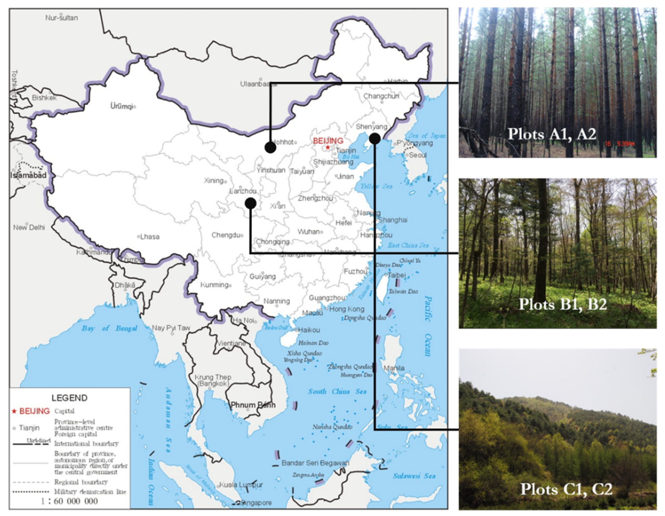
Six long-term positioning forest plots of 100 × 100 m2 were analyzed (Table 1). All trees with DBH greater than or equal to 5 cm were labeled. Tree coordinates, species, DBH, height, crown were recorded by a total station (a Total station-G.T.S. 602AF, Topcon Sokki Co., Ltd, Tokyo, Japan). These natural forests were located in different regions of China (Figure 1). Plots A1 and A2 were Pinus sylvestris forests in the sandy land north of the temperate zone, established in 2015. Plots B1 and B2 were mixed forests of pinus and quercus in the transition zone from subtropical to warm temperate zone, established in 2009. Plots C1 and C2 were mixed forests of Pinus koraiensis and broad-leaf forests in the central temperate zone, established in 2002.

Table 1.
Details of the plots.

Figure 1.
Location of the six plots.
Plots A1 and A2 were located in the southern Hulunbuir desert. They belong to the middle western slope of Greater Khingan Range, a transition zone stretching to the Inner Mongolia plateau (47°36′35″–48° N, 118°58′–120°32′ E), elevation 700–1100 m, in temperate semi-humid and semi-arid continental monsoon climate, with annual average temperature 1.5 °C and an average yearly rainfall of 344 mm. The soil type was mainly sandy soil. The forest type was pure forests of Pinus sylvestris var.mongolica Litv.
Plots B1 and B2 were located in Xiaolongshan, Gansu province (33°30′–34°49′ N, 104°43′22″–106° E), and they were in the transition zone from subtropical to warm temperate. The elevation was about 1000 m with an annual average temperature of 7–12 °C and an annual average rainfall of 800 mm. The soil was mountainous brown soil, which was moist and rich in organic matter. The forests were mixed forests of pinus and quercus. The main broad-leaf tree species were Quercus aliena var. acuteserrata Maxim. and Quercus liaotungensis Koidz. The main conifer species were Pinus armandi Franch. and Pinus tabulaeformis Carr., accompanied by Populus davidiana Dode., Toxicodendron verniciflum F.A.Berkley, Populus purdomii Rehd., Tilia paucicostata Maxim., Carpinus cordata Bl., Crataegus kansuensis Wils., and Kalopanax septemlobus Koidz., etc.
Plots C1 and C2 were located in the east slope of Jiaohe Forestry Bureau of experimental area, Jilin province (43°51′–44°05′ N, 127°35′–127°51′ E). The elevation was 400–500 m. The climate was temperate continental monsoon climate, with an annual average temperature of 3.5 °C and annual rainfall between 700 and 800 mm. The soil type was dark brown soil of higher fertility. The forests were mixed Pinus koraiensis and broad-leaf forests, and the main conifer species were Pinus koraiensis Sieb. et Zucc. and Abies holophylla Maxim; the main broad-leaf tree species are: Fraxinus mandshurica Rupr., Juglans mandshurica Maxim, Acer mandshurica Maxim., Carpinus cordata, Tilia mandschurica Rupr. et Maxim, Quercus mongolica Fisch.
3. Methods
3.1. Definition of Random Trees
According to the uniform angle index values, individuals were categorized as even, random, and clustered trees [18].
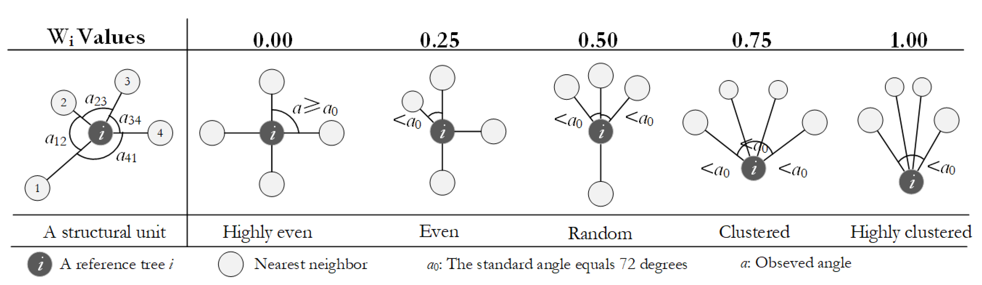
We utilized the uniform angle index to describe the uniformity of the nearest neighbors of a reference tree i (the observed tree in a structural unit), see Figure 2. We measured the angles (α) of two adjacent neighbors and i and compared with a standard angle (α0, α0 = 72° with four neighbors) to analyze the distribution of the neighbors [11,20]. It was defined as the ratio of the number of α angles less than the standard angle α0 among the four nearest neighbors, see Formula (1):
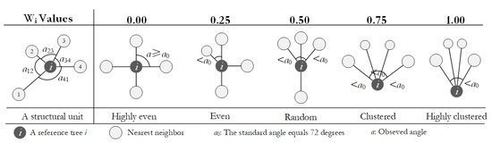
Figure 2.
A structural unit and the principle of the uniform angle index.
Wi can assume five discrete values. The four neighbors and the reference tree named a structural unit for convenience. The structural unit was an even structural unit if Wi = 0 or 0.25. The reference tree was an even tree. The structural unit was a clustered structural unit if Wi = 0.75 or 1. The reference tree was a clustered tree. The structural unit was a random structural unit if Wi = 0.5. The reference tree was a random tree [18].
3.2. Community Characteristics
We analyzed key variables of natural forests, including tree species composition (abundance distribution), stand structure (diameter distribution, Voronoi polygon side distribution, mingling degree distribution, crowding degree distribution), and tree competition (competition degree distribution).
3.2.1. Species-Abundance Distribution
The distribution shows tree species composition in a natural forest, with the Y-axis, represents the frequency of different species and the X-axis tree species.
3.2.2. Diameter Distribution
The study used the equal-diameter classes to show the DBH distribution of the stand. The X-axis indicates tree diameters with 2 cm intervals in the order from small to big. The Y-axis indicates the frequency of tree numbers corresponding to each diameter class.
3.2.3. Voronoi Polygon Side Distribution
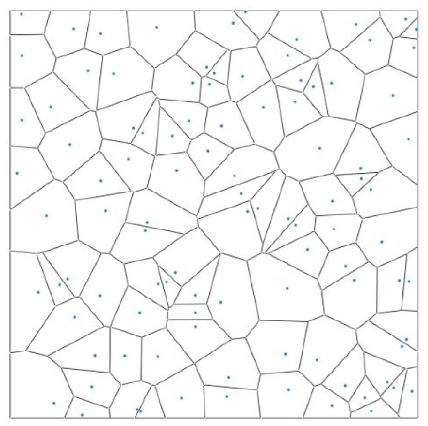
The Voronoi diagram is a popular tool to describe the spatial structure of tree patterns. It calculates the effective influence range of the points according to their discrete distribution. The Voronoi diagram segmentation algorithm has been widely used in various fields and successfully applied in analyzing the number of competitive trees recently (Figure 3). Different forest tree patterns possess certain variation regularity in their Voronoi diagrams. The standard deviations of the mean value show distinct differences [21]. The range of randomly distributed forests was Sv: [1.264, 1.402]. If Sv < 1.264, the forest was an even spatial pattern; if Sv > 1.402, it was clustered.
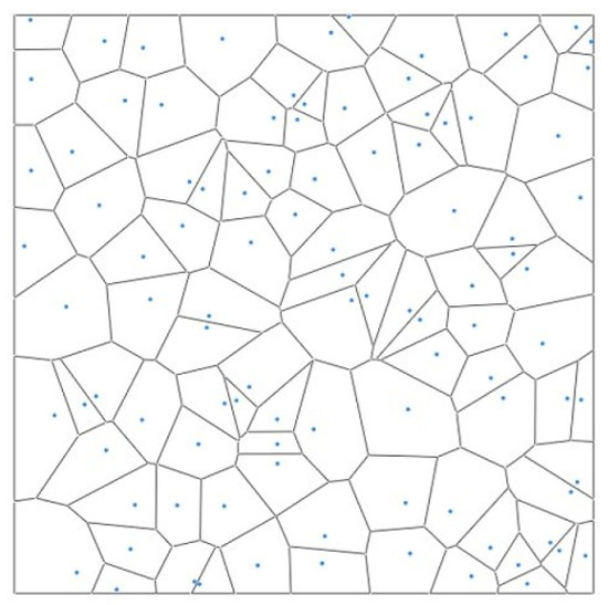
Figure 3.
Schematic diagram of Voronoi polygon.
3.2.4. Mingling Degree Distribution
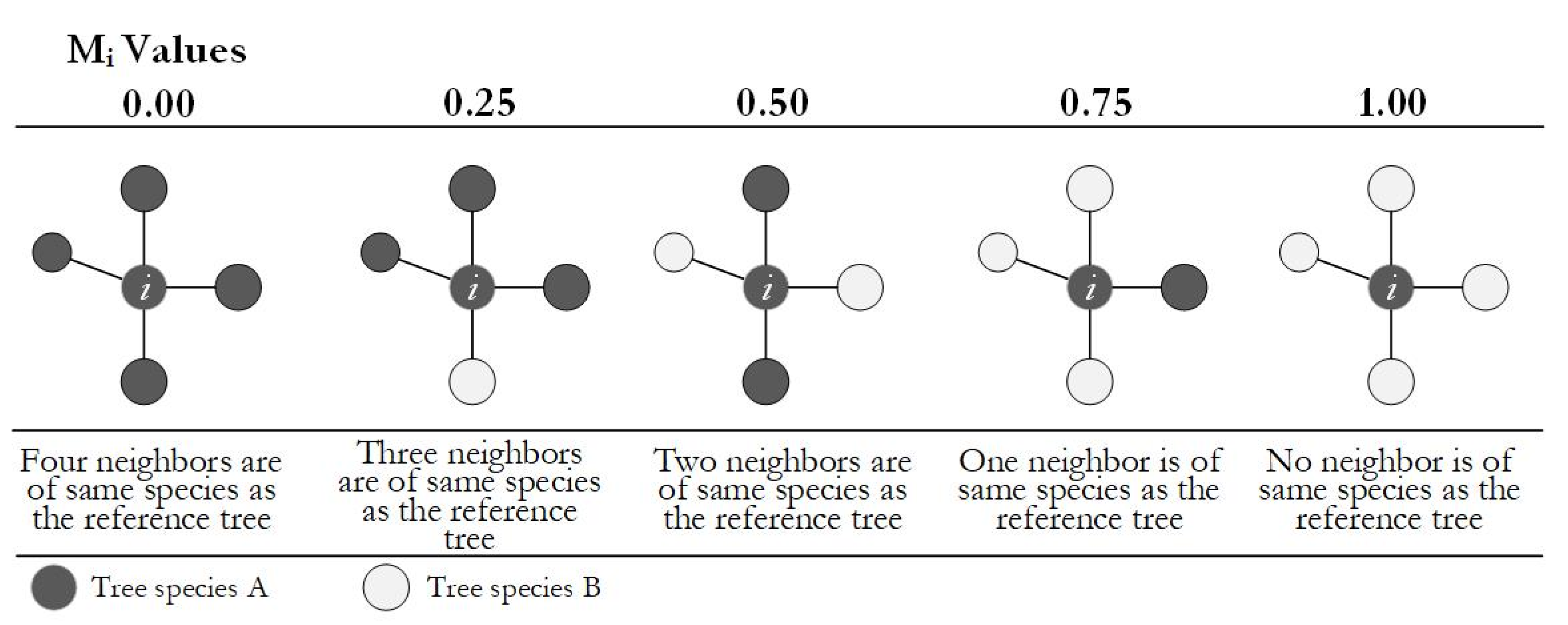
Mingling degree (Mi) indicates the spatial isolation degree of species in mixed forests [5]. It was defined as the proportion of trees that were not of the same species as the reference tree in the four nearest neighbor trees, see Formula (2):
The Mingling degree depicts the probability that the nearest neighbor of any reference tree is of different species [22]. Mi assumes five values, as shown in Figure 4.
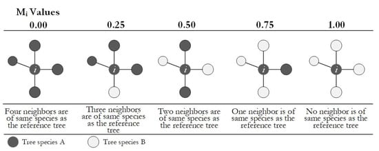
Figure 4.
Principle of the mingling.
Five possible values correspond to five degrees of mingling: zero, weak, medium, strong, and extremely strong, indicating the degree of isolation of tree species in a structural unit.
3.2.5. Crowding Degree Distribution
Crowding degree (Ci) was defined as the ratio of trees among the four nearest neighbors connected crowns with the reference tree [22]. Crown connectivity refers to the full or partial connection of horizontal projections of the canopy. Tangential or independent crowns were not qualified as crown connectivity. See Formula (3):
Crowding degree analyzes the forest crowding and local density based on the crown connection degree in a structural unit. Ci assumes five values, as shown in Figure 5.
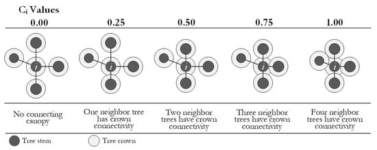
Figure 5.
Principle of the crowding degree.
3.2.6. Competition Distribution
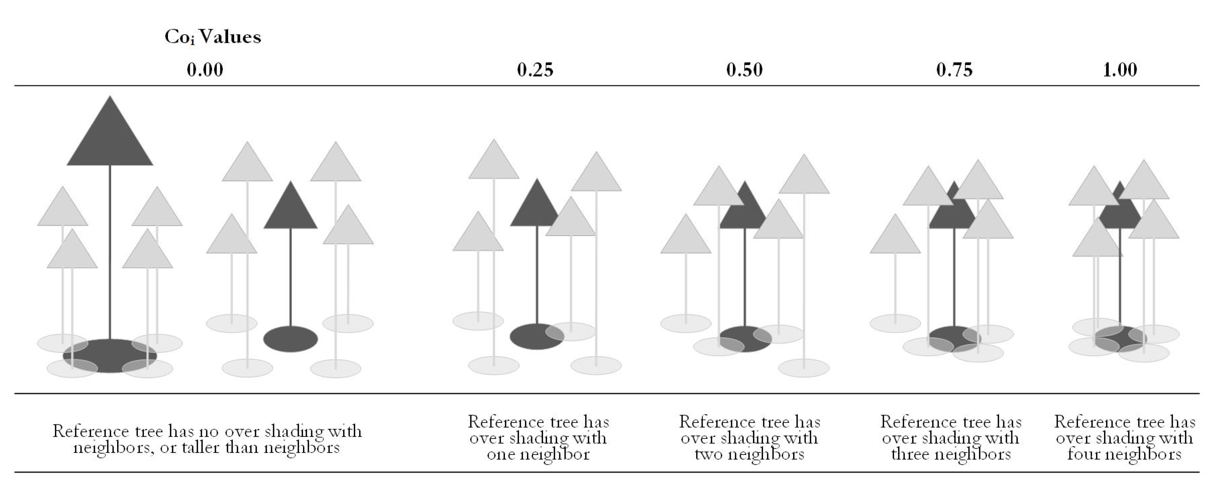
Forest tree competition (Coi) was used to express individual competition. The degree of competition represents the degree of the crown over shading, which was calculated by referring to the number of trees among the four nearest neighbor trees that have a crown cover over the reference tree i. Canopy cover refers to the full or partial overshading of the two trees’ crowns (total or partial overlap), while the neighbor tree height was higher than the reference tree. A tangential or independent canopy was not qualified as a crown cover. See Formula (4):
The competition degree analyzed the forest competition based on the structural unit. Ci assumes five values. See Figure 6.
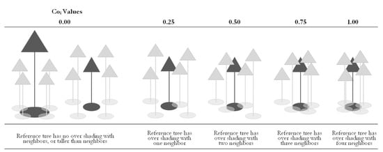
Figure 6.
Principle of the competition degree.
3.3. Similarity Test
The difference in community structure composition was measured by the genetic absolute distance method [23,24,25,26]. This method can compare differences between two populations or communities to identify whether two distributions come from the same population. This method was widely applied to compare stand diameter distributions because it can give the specific difference value between the two distributions. See Formula (5).
where xi is the frequency of genetic type i in community X; yi is the frequency of genetic type i in community Y. k is the number of genetic types. Based on the analysis of the possibility of applying genetic distance to community structure comparison, Hui et al. [27] proposed the critical value for a significant difference in Formulas (6–7). When the difference between the two distributions, the difference was considered significant, and thus we cannot say they are coming from the same population. Conversely, the two distributions were considered similar.
where dmax is the larger genetic distance obtained when X and Y distributions are compared with the uniform distribution Z, respectively. The significance test was performed on the confidence level α = 0.05.
4. Results
4.1. Tree Species Composition
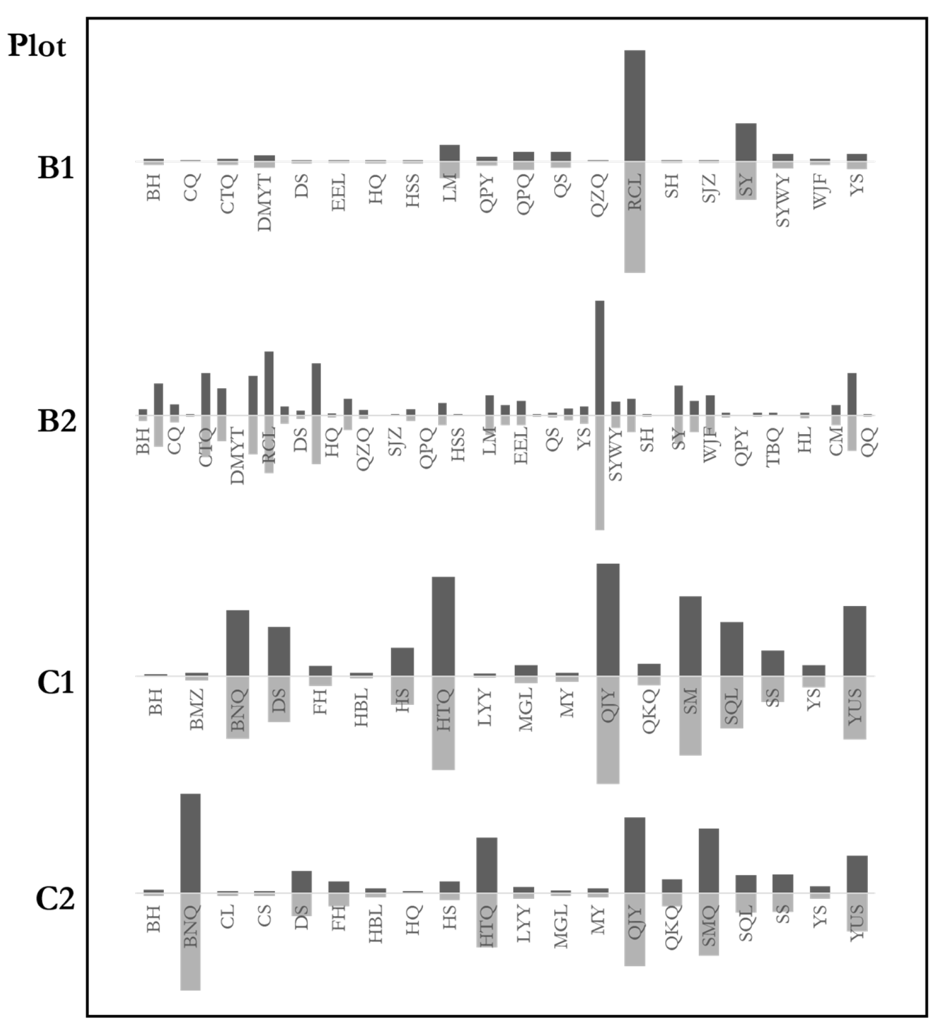
Tree species abundance distribution reflects tree species composition. We studied the species abundance of both natural mixed forest communities and random trees. The communities and the random trees had similar species abundance distributions (Figure 7). The figure demonstrates the percentage of certain species in the communities and the random trees. The similarity of the characteristics between random trees and communities was also analyzed for further study. The genetic distance test results were: B1: ; B2: ; C1; C2. The result indicates that the species composition of the forest communities was highly similar to the random trees. The maximum difference of the four plots was 6%, far from the significant difference. The species abundance distributions of random trees fully reflect the species composition of natural mixed forests.
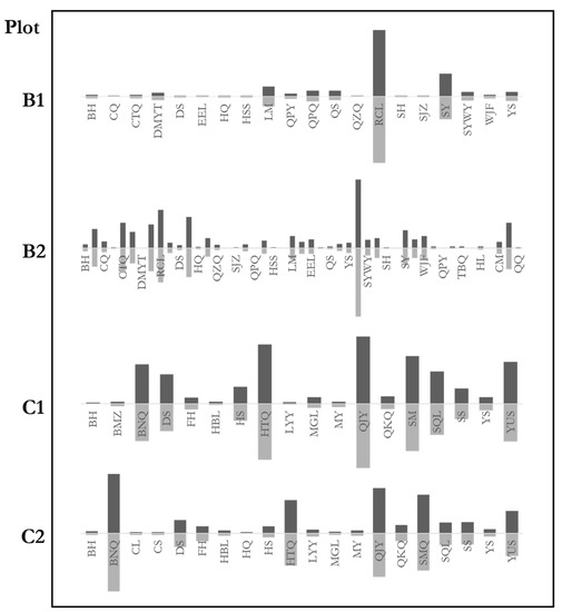
Figure 7.
Abundance distributions of stands and random trees. Distributions of the stands are above the horizontal axes. Distributions of the random trees are below the horizontal axes. Species of C2 are not all listed to save space. BH, Betula platyphylla Suk.; CQ, Kalopanax septemlobus (Thunb.) Koidz.; CTQ, Acer ginnala Maxim.; DMYT, Cerasus polytricha; DS, Tilia mongolica Maxim.; EEL, Carpinus turczaninowii Hance; HQ, Sorbus pohuashanensis (Hance) Hedl.; HSS, Pinus armandii Franch.; LM, Swida macrophylla (Wall.); QPY, Acer cappadocicum Gled.; QPQ, Populus cathayana var. cathayana; QS, Toxicodendron vernicifluum (Stokes) F.A. Barkley; QZQ, Acer davidii Franch.; RCL, Quercus aliena var. acutiserrata Maxim.; SY, Populus davidiana Dode; SYWY, Lindera obtusiloba Bl.; WJF, Acer oliverianum Pax; YS, Populus tomentosa Carr.; TBQ, Acer caesium Wall.; HL, Salix cheilophila var. microstachyoides; CM, Aralia chinensis Linn.; QQ, Picea wilsonii Mast.; SH, Betula delavayi; SJZ, Malus baccata (Linn.) Borkh.; BMZ, Syringa reticulata (Bl.) Hara var. Mandshurica (Maxim.) Hara (S. Amurensis Rupr.); BNQ, Acer mandshuricum Maxim.; DS, Tilia mongolica Maxim.; FH, Betula costata Trautv.; HBL, Phellodendron amurense Rupr.; HS, Pinus koraiensis; HTQ, Juglans mandshurica; LYY, Ulmus laciniata (Trautv.) Mayr; MGL, Quercusmongolica Fischer ex Ledebour; MY, Ostrya japonica Sarg.; QUY, Carpinus cordata Bl.; QKQ, Acer tegmentosum Maxim.; SM, Acer mono Maxim.; SQL, Fraxinus mandschurica Rupr.; SS, Abies holophylla Maxim.; YUS, Ulmus pumila Linn.
4.2. Stand Structure
4.2.1. Diameter Distributions
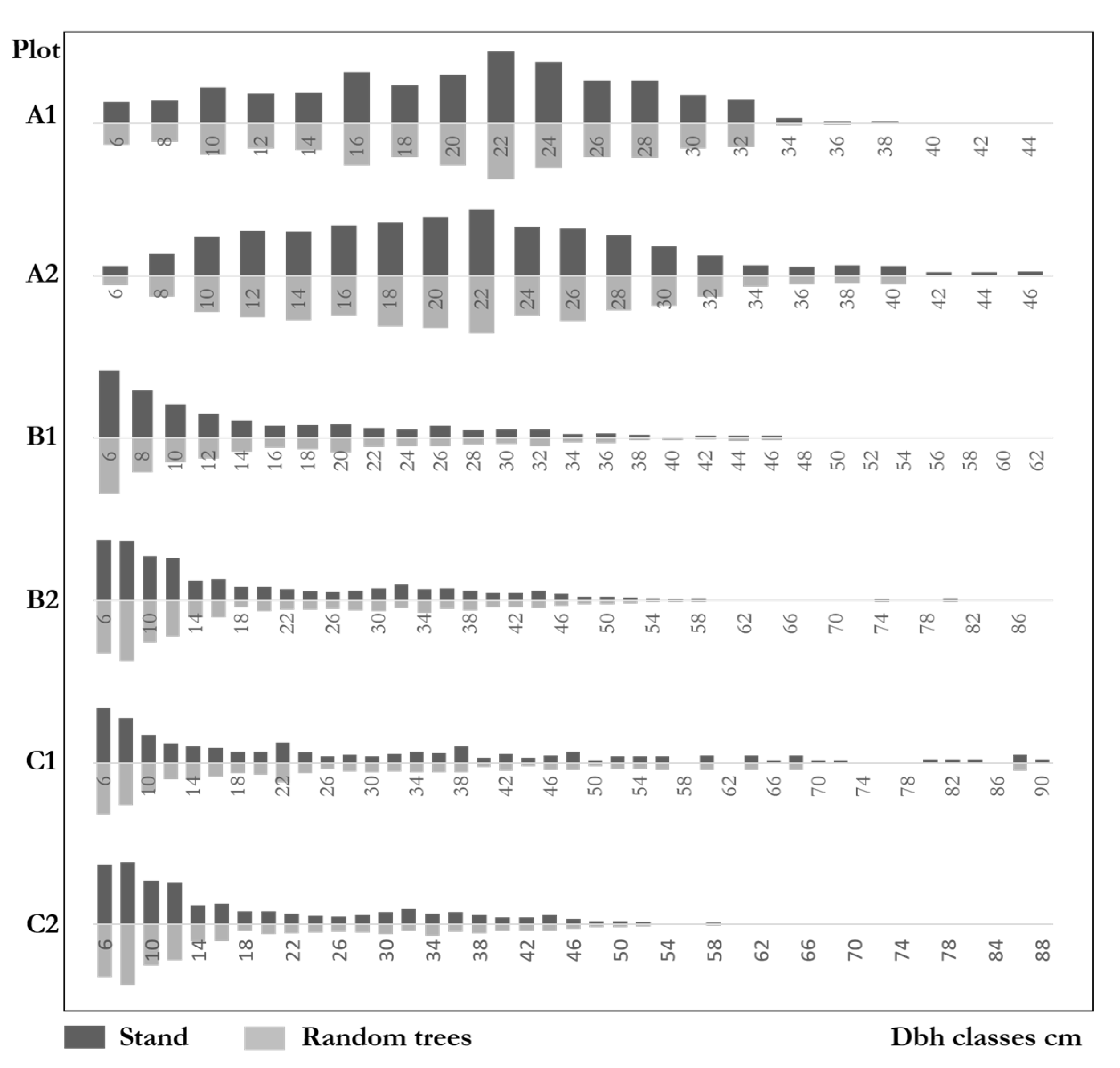
Figure 8 shows the diameter distributions of natural forests and random trees. The distributions of both communities and the random trees were very similar. Furthermore, the ratios of each diameter class on the community level were highly similar to those of random trees. The genetic distance test results of the six plots were: A1: ; A2: ; B1: ; B2; C1; C2. The results indicate that the diameter distributions of random trees were very similar to that of the communities. The maximum difference of the six plots was 10.8%, which was far from the significant difference. The diameter distributions of random trees fully reflect the size distributions in natural forests.
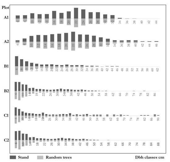
Figure 8.
Diameter distributions of stands and random trees.
4.2.2. Pattern Distributions
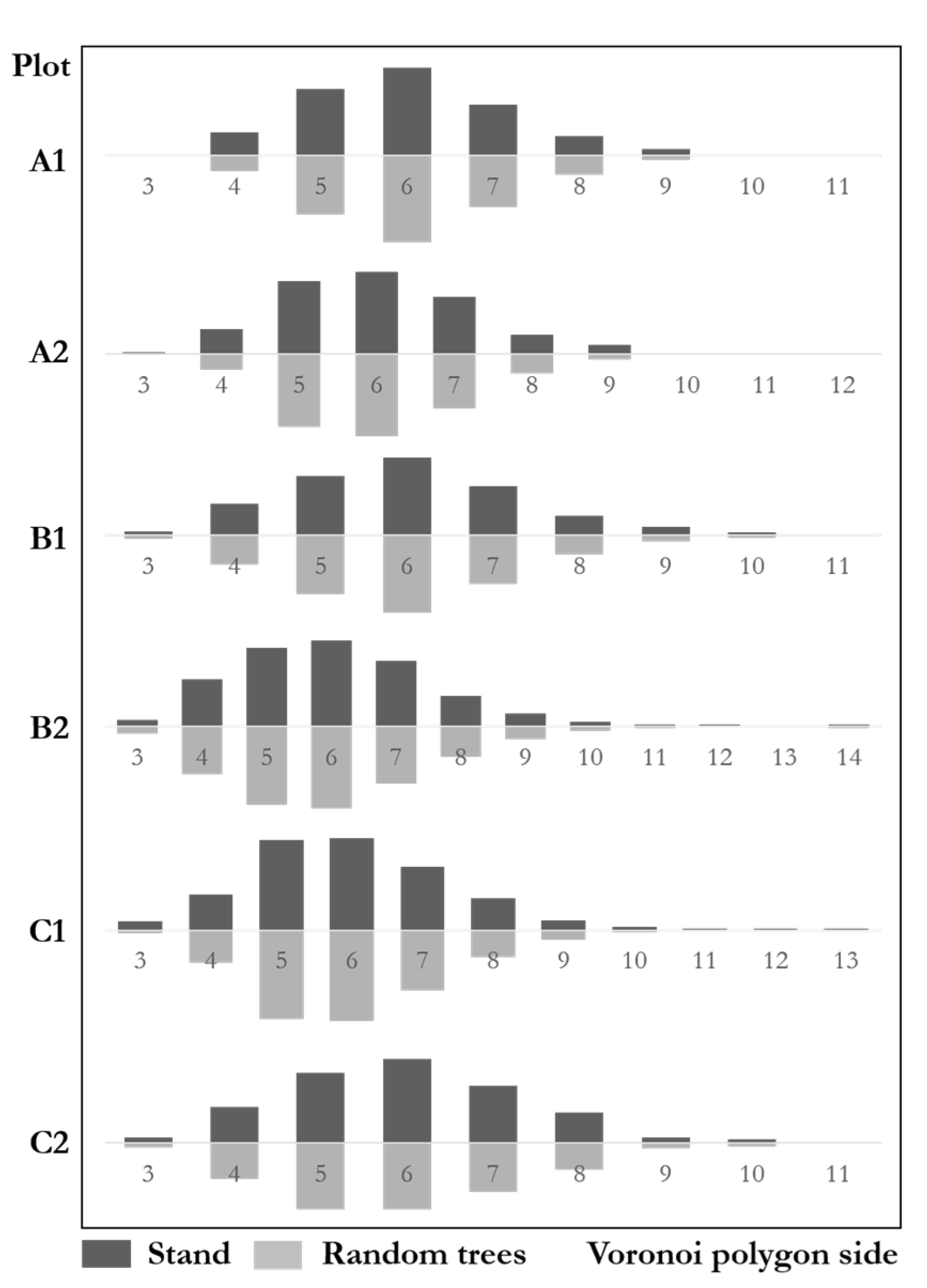
Figure 9 shows the Voronoi polygon side distributions with similar results between communities and the random trees. The genetic distance test of the six plots was: A1 ; A2; B1 ; B2: ; C1; C2. The result shows that the distributions of both communities and random trees were highly similar. The maximum difference of six plots was 6.8%, far from the significant difference.

Figure 9.
Voronoi polygon side distributions of stands and random trees.
According to the Sv analysis, A1 (Sv = 1.242), A2 (Sv = 1.256) were uniformly patterns. B1 (Sv = 1.401) was a random pattern. B2 (Sv = 1.677), C1 (Sv = 1.563) and C2 (Sv = 1.406) were clustered. Sv analysis of random trees A1 (Sv = 1.169), A2 (Sv = 1.153) were uniformly patterns. B1 (Sv = 1.400) was random. B2 (Sv = 1.737), C1 (Sv = 1.574) and C2 (Sv = 1.436) were clustered. The results suggest that random trees and the stands were highly similar. The random trees fully reflect the spatial pattern of natural forests.
4.2.3. Mingling Degree Distributions
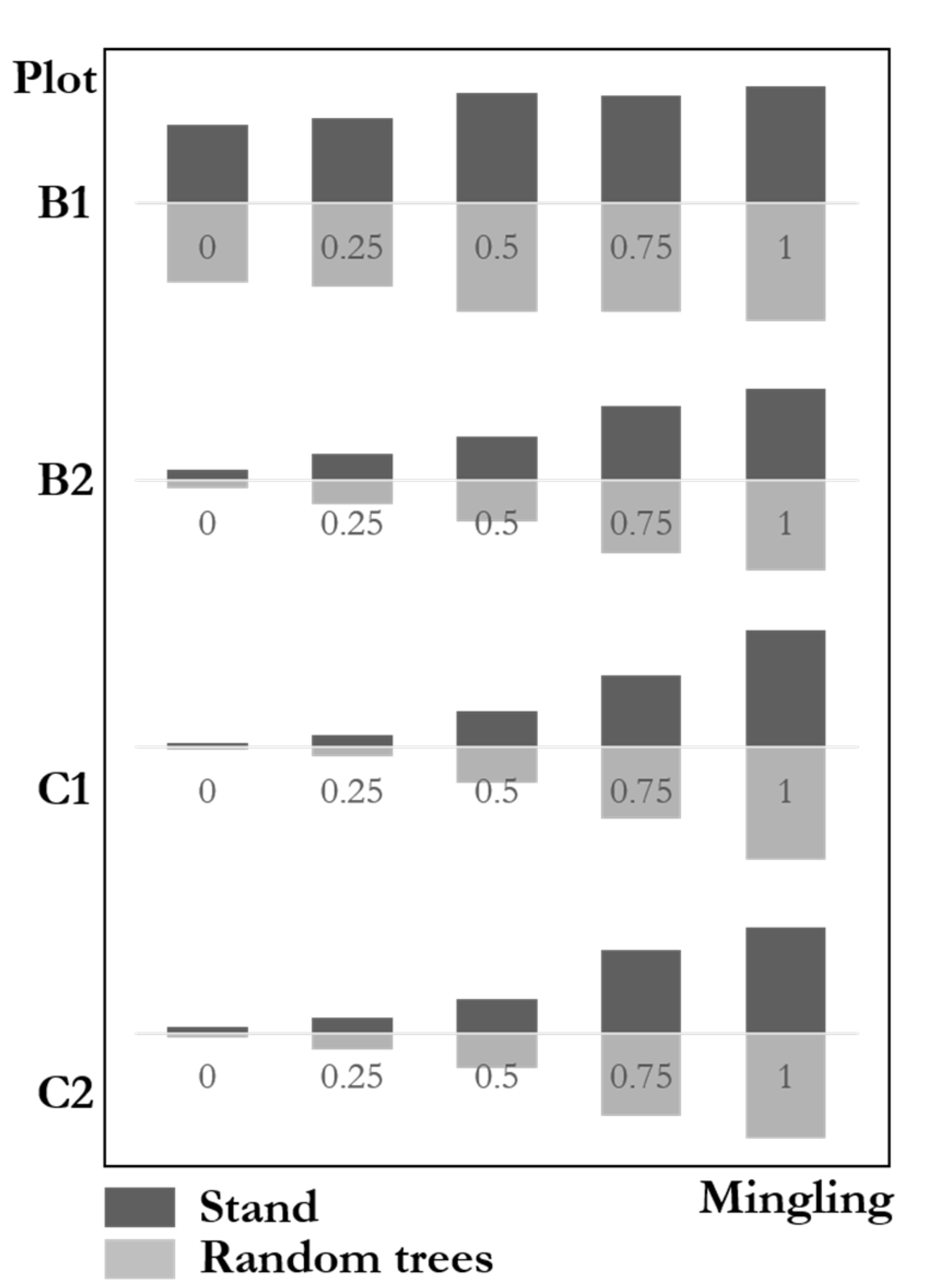
Figure 10 shows the mingling degree distributions between communities and the random trees with highly similar results. The frequencies of high mingling, medium mingling, and low mingling in communities were highly similar to those in random trees. The genetic distance test results of four natural mixed forest plots were: B1 ; B2; C1; C2. This result indicates that the species mingling degree of random trees was highly consistent with that of the communities. The maximum difference of the four plots was less than 3%, far from the significant difference. The species isolation of random trees fully reflects that of the communities.

Figure 10.
Mingling degree distributions of stands and random trees.
4.2.4. Crowding Degree Distributions
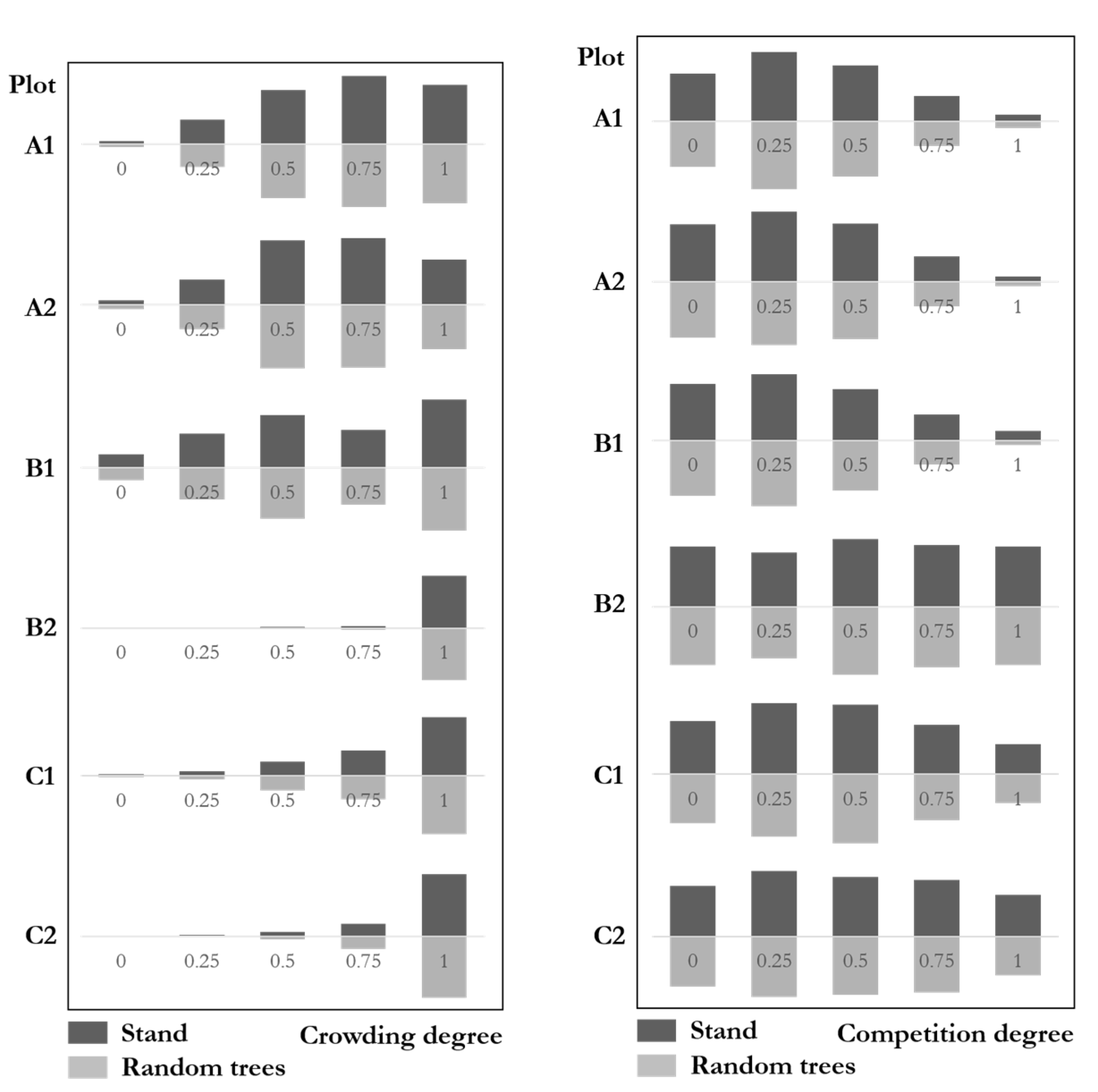
Figure 11 (left) shows the crowding degree distributions with similar results between stands and the random trees. The genetic distance test results of the six plots were: A1: ; A2; B1 ; B2; C1; C2: . This result indicates that the crowding degree distributions of random trees were very similar to that of the communities. The maximum difference of all six plots was 4%, which was far from the significant difference. The crowding degree of random trees fully reflects that of the communities.
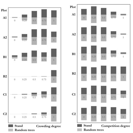
Figure 11.
Crowding degree (left) and competition degree (right) distributions of stands and random trees.
4.3. Tree Competition
Figure 11 (right) shows the competition degree distributions with similar results between stands and random trees. The genetic distance test results of the six plots were: A1 ; A2; B1 ; B2; C1; C2. This result indicates that the competition degrees of random trees were very similar to that of the communities. The maximum difference of all six plots was 3.3%, far from the significant difference. The competition degree distributions of random trees fully reflect that of natural forest communities.
5. Discussion
5.1. Proportion of Random Trees in Distributions
Except for plots A1 and A2, which were single species forests, others were mixed forests. The similarity of tree species composition between communities and random trees shows that random trees appear in most tree species with a similar proportion (Figure 7). For example, the proportion of random trees of each species was about 50% in plot B2, in which 47 species were reported. The balance of random trees in the communities is maintained at a particular proportion since each species has a similar ratio of random trees, which leads to the similarity of species distributions between the random trees and the communities.
As for the DBH distributions, we noticed that plots B1, B2, C1, and C2 were inverted order distributions. The number of trees concentrates at the smallest class and decreases sharply with the DBH increases, which shows a typical uneven-aged forest structure. Plots A1 and A2 were approximately normal distributions, with the largest number of trees in the diameter class where the average DBH was located. Trees then gradually decreased in other diameter classes to both sides, a typical even-aged forest structure. Since the small trees tended to be clustered with their neighbors [28,29] and the random trees have competitive advantages (see Section 5.2.), we inferred that the proportion of random trees would increase when DBH increases, particularly in the uneven-aged forests with long-term development. However, we did not confirm this idea in our result. The distributions are the same as the communities in all plots. The proportion of random trees do not seem to be affected by the increase of DBH. In other words, individuals of different sizes are formed by random trees with a particular ratio. This may be because only trees with DBH greater than or equal to 5 cm were reported in the forests.
We then used the crowding degree to express the local density of individuals. Random trees usually show a similar ratio with the communities. We noticed plot A2 shows a small difference (Figure 11, left). Crowding = 0.75 is greater than that of 0.5 in stand-level, while it shows an opposite result in the random trees. Although the results did not present a more evident decrease in crowding or competition in other plots, and the similarity test is significantly similar between the random trees and communities, whether random trees can show less crowding and competition are worth further study.
5.2. The Quantity Advantage of Random Trees
Different spatial patterns may bring about the density-dependent mortality caused by competition with neighboring individuals [30,31,32], which leads to the differentiation of individuals over time and influences forest dynamics [33,34]. Few studies on the classification of forest trees are based on the concept of spatial patterns [18,19,35]. The uniform angle index quantitatively describes the spatial distribution of the nearest neighbors of a reference tree [20,36], which spatially reflects the relationship between adjacent trees and a references tree in different directions [37]. Therefore, the essence of classification based on the uniform angle index describes the competition in space.
The quantity advantage of structural units can also be further explained using competition relationships. For example (Figure 12), neighbor trees are crowded together in a clustered unit. The reference tree receives light from three sides, occupies more space, showing a larger canopy and higher productivity [38]. Asymmetric competition between large and small neighbor trees may lead to asymmetric competition [39,40,41]. At the same time, the local density between neighbors is high, intensifying the competition as well. Both competitions may reduce the growth of neighbors and eventually to the mortality of trees that are not successful competitors [42,43,44]. Then the clustered structural unit disintegrates, the remaining trees reintegrate with other trees to form a new structural unit. The stronger the aggregation, the more probabilities of disintegrating and reintegrate.

Figure 12.
Disintegration–reintegration process of different structural units. Numbers present the proportion of varying structural units in natural forests.
On the contrary, in an even structural unit, the reference tree is under competition from three or four directions. The extrusion and coverage of the neighbor trees may eliminate weak reference trees. Then, the even structural unit may disintegrate. The remaining trees reintegrate with other trees to form a new structural unit. The more crowded and regular the trees are, the more probabilities to disintegrate and reintegrate.
The random tree obtains more light from two sides and assumes less competition than an even tree. Neighbors in a random structural unit suffer less extrusion and overshading with each other than neighbors in a clustered unit. Therefore, both random trees and their neighbors bear less pressure with low probabilities to be weak or unhealthy. Thus, random structural units have a higher possibility to grow steadily with a higher survival rate in natural succession.
Contingent factors such as distance and unhealthy trees reducing the competition of non-random structural units cannot be ignored. However, these are limited cases. At the same time, random structural units may obtain more probabilities to stay in long-term stability and are not easy to disintegrate. Random structural units effectively provide a more stable environment to maintain a dynamic balance of the forest. Therefore, in a well-developed natural community, random structural units constitute the majority. In contrast, the even and clustered structural units remain within a particular proportion. Extreme structural units (very regular or very aggregative) are very few (<5%). The mean value of such stands tends to be 0.5, which indicates this balance [21]. When severe natural disasters, diseases, and forest insects, or human disturbance, the balance of forest spatial structure may be broken, non-random structural units may increase. These non-random structural units would gradually disintegrate and reintegrate in the natural selection over decades to complete the natural restoration and rehabilitation. With fewer non-random structural units, increased random structural units resume and maintain such dynamic balance again.
We call the above hypothesis the disintegration–reintegration process, explaining why the random structural units are the primary component in natural forests. In general, random trees are easier to survive and maybe have a higher growth rate than others, which becomes a quantitative advantage. The individual size or growth rate should be analyzed for further demonstration. However, it is challenging to observe the process of a single structural unit in a natural forest because of the influence of regeneration, ecological interactions, and other interferences. In this case, a controlled experiment may be a feasible alternative method for a further study.
5.3. The Quantity Advantage Makes the Random Trees Consistent with the Community Characteristics
The quantity advantage of random trees may explain our results. We counted the percentages of random trees in the six plots: A1: 59.2%; A2: 59.3%; B1: 56.2%; B2: 53.5%; C1: 55.0%; C2: 56.7%. This result shows the same with Zhang et al. [18], which reported that random trees are the majority accounting for more than a half.
The even and clustered trees count for only the small half of the communities. Here, we analyzed the above parameters of even and clustered trees to compare better (Table 2). The results proved that, although the Voronoi polygon side distribution did not reach a significant level, the pattern difference illustrated by the Sv was huge. Four plots were inconsistent with the statistical results of the forests. The Sv of even trees in B1 was 1.414, which was a clustered pattern. The Sv of the forest was 1.401, which suggested random. The Sv of even trees in C2 was 1.287, a random pattern, while the Sv of the forest was 1.436, which meant clustered. The forest Sv of A2 and C1 were 1.256 and 1.563, which indicated even and clustered, respectively, while the Sv of clustered trees showed a random pattern (A2: 1.290; C1: 1.394). In terms of the degree of species isolation, B1 was significantly different from the statistical results of the stand. As for the competition degree, two plots (B2 and C2) were significantly different from those of the forests. None of the even or clustered trees fully present the community characteristics. The bold numbers provide different results between the even/clustered trees and the communities in Table 2.
Table 2.
Similarity test of even and clustered trees with the stands and the Sv results. (; * indicates significant difference).
We notice that only random trees correctly reflect the characteristics of the communities. The proportion of random trees determines its consistency with the communities. It is not so much that the random trees reflect the characteristics of natural forests as that the random trees are the main components of natural forests, which together with a small number of aggregates and even structure units constitute the natural forest. Therefore, the characteristics of natural forests are often dominated by random trees.
5.4. Forest Types
Interestingly, this result does not illustrate a correlation with a particular forest type. The six natural forest plots analyzed in this study were distributed in three northern regions of China with different climates and developed in various conditions (Table 1). For example, four plots are composed of about 20 species (B1, C1, and C2) and 47 (B2). The abundance and mingling between the random trees and the communities were similar, respectively. Plots A1 and A2 were regenerated after the forest fire. The individuals were distributed evenly in the forests, while plots B1 and C1 were random, and others were aggregated. However, the spatial patterns were consistent between the random trees and the communities in different patterns. These results elucidate that the similarity between the random trees and the communities is not related to the forest types, which is the same as previous researches [18].
However, a new-built artificial forest may not display this characteristic. Mainly the forest appears as symmetric arrangements with low structure diversity [19]. Artificially increasing the proportion of random trees in plantations to create asymmetric competition could raise the spatial structure heterogeneity and accelerate the near-natural transformation of plantations, which is also one of the applications of this study.
6. Conclusions
This study compared the key characteristics of random trees and tested the similarity with those of the communities, such as tree species composition (abundance), stand structure (diameter distribution, Voronoi polygon side distribution, mingling degree distribution, crowding degree distribution), and trees competition (competition degree distribution). The random trees in six plots demonstrated the high similarity of all the key parameters with the communities. The genetic absolute distance method was applied to further corroborate the similarity of the random trees and the stands, with a significance level of 0.05. Therefore, this study supports our hypothesis and proves that random trees present several features of the natural communities.
The spatial pattern of forests covers a wide range and requires sufficient observation [45]. It is necessary to investigate individual tree characteristics and location information to better understand the dominant trees’ ecological process [46], which requires many human resources and time costs. At present, the investigation is often limited to a sub-plot. It requires that this sub-plot can represent or fully express the overall characteristics of the stand in all aspects [47]. Achieving accurate forest attributes and structures efficiently regarding time and cost for fieldwork is controversial in forest science [48,49]. This study proved that random trees represent natural forests in quantity and characteristics. This group carries the information of a natural forest in all aspects, which accurately reflect the overall tree species composition, stand structure, and competition, etc.
Therefore, targeting random trees in natural forests can significantly improve research efficiency, protection, management, and monitoring of forest resources. For example, in the natural forest protection, random trees of key species can be selected as key individuals for conservation monitoring. In the study of forest eco-hydrological, random trees can be adopted as the monitoring object. In the study of climate dendrochronology and forest yield, random trees can be used as sampling objects. In silviculture, plantation forests can be established, adjusted, or tended in line with random forest characteristics in natural forests. Random tree study instills new ideas to forest science, including stand research and forest survey techniques.
Author Contributions
Conceptualization, G.Z. and G.H.; methodology, G.H.; software, formal analysis, writing—original draft preparation and visualization, G.Z.; writing—review and editing, funding acquisition, G.H. All authors have read and agreed to the published version of the manuscript.
Funding
This work was supported by the National Key Research and Development Program of China, grant number 2016YFD0600203.
Data Availability Statement
Not applicable.
Conflicts of Interest
The authors declare no conflict of interest.
References
- FAO. Global Forest Resources Assessment; Food and Agriculture Organization of the United Nations, FAO: Rome, Italy; Quebec City, QC, Canada, 2015. [Google Scholar]
- Keenan, R.J.; Reams, G.A.; Achard, F.; de Freitas, J.V.; Grainger, A.; Lindquist, E. Dynamics of global forest area: Results from the FAO Global Forest Resources Assessment 2015. For. Ecol. Manag. 2015, 352, 9–20. [Google Scholar] [CrossRef]
- Tang, S.; Feng, Y.; Hong, L.; Du, J. Design and application of natural forest resource data updating on the basis of power builder. For. Res. 2000, 13, 439–442. (In Chinese) [Google Scholar]
- Corral-Rivas, J.J.; Wehenkel, C.; Castellanos-Bocaz, H.A.; Vargas-Larreta, B.; Diéguez-Aranda, U. A permutation test of spatial randomness: Application to nearest neighbour indices in forest stands. J. For. Res. 2010, 15, 218–225. [Google Scholar] [CrossRef]
- von Gadow, K.; Zhang, C.Y.; Wehenkel, C.; Pommerening, A.; Corral-Rivas, J.; Korol, M.; Myklush, S.; Hui, G.Y.; Kiviste, A.; Zhao, X.H. Forest structure and diversity. In Continuous Cover Forestry, 2nd ed.; Pukkala, T., von Gadow, K., Eds.; Managing Forest Ecosystems 23; Springer: Dordrecht, The Netherlands, 2012; pp. 29–83. [Google Scholar]
- Aguirre, O.; Hui, G.; von Gadow, K.; Jiménez, J. An analysis of spatial forest structure using neighbourhood-based variables. For. Ecol. Manag. 2003, 183, 137–145. [Google Scholar] [CrossRef]
- Wiegand, T.; Moloney, K.A. A Handbook of Spatial Point Pattern Analysis in Ecology; CRC Press: Boca Raton, FL, USA, 2014. [Google Scholar]
- Ripley, B.D. Modelling Spatial Patterns. J. Royal Stat. Soc. 1977, 39, 172–212. [Google Scholar] [CrossRef]
- Clark, P.J.; Evans, F.C. Distance to nearest neighbor as a measure of spatial relationships in populations. Ecology 1954, 35, 213–227. [Google Scholar] [CrossRef]
- Pommerening, A.; Grabarnik, P. Individual-based methods in forest ecology and management; Springer: Cham, Switzerland, 2019. [Google Scholar]
- Hui, G.; Gadow, K. Das Winkelmass—Theoretische Überlegungen zum optimalen Standardwinkel. Allg. Forst Jagdztg. 2002, 173, 173–177. [Google Scholar]
- Hui, G. Stichprobensimulationen zur Schätzung nachbarschaftsbezogener Strukturparameter in Waldbeständen. Allg. Forst Jagdztg. 2004, 175, 199–209. [Google Scholar]
- Hui, G.; Abert, M.; von Gadow, K. Das Umgebungsmaß als Parameter zur Nachbildung von Bestandesstrukturen. Forstwiss. Cent. Ver. Tharandter Forstl. Jahrb. 1998, 117, 258–266. [Google Scholar] [CrossRef]
- Li, Y.; Hui, G.; Zhao, Z.; Hu, Y. The bivariate distribution characteristics of spatial structure in natural Korean pine broad-leaved forest. J. Veg. Sci. 2012, 23, 1180–1190. [Google Scholar] [CrossRef]
- Pommerening, A. Evaluating structural indices by reversing forest structural analysis. For. Ecol. Manag. 2006, 224, 266–277. [Google Scholar] [CrossRef]
- Graz, F.P. Spatial diversity of dry savanna woodlands: Assessing the spatial diversity of a dry savanna woodland stand in northern Namibia using neighbourhood-based measures. Biodivers. Conserv. 2004, 15, 1–16. [Google Scholar] [CrossRef]
- Zhao, Z.; Hui, G.; Hu, Y.; Wang, H.; Zhang, G.; von Gadow, K. Testing the Significance of different Tree Spatial Distribution Patterns based on the Uniform Angle Index. Canadian J. For. Res. 2014, 44, 1417–1425. [Google Scholar] [CrossRef]
- Zhang, G.; Hui, G.; Zhao, Z.; Hu, Y.; Wang, H.; Liu, W.; Zang, R. Composition of basal area in natural forests based on the uniform angle index. Ecol. Inf. 2018, 45, 1–8. [Google Scholar] [CrossRef]
- Zhang, G.; Hui, G.; Hu, Y.; Zhao, Z.; Guan, X.; Gadow, K.; Zhang, G. Designing near-natural planting patterns for plantation forests in China. For. Ecosyst. 2019, 6. [Google Scholar] [CrossRef] [Green Version]
- Gadow, K.; Albert, M.; Hui, G. Das Winkelmaß—Ein Strukturparameter zur beschreibung der Individualverteilung in Waldbeständen. Centralblatt für das gesamte Forstwesen. Cent. Gesamte Forstwes 1998, 115, 1–10. [Google Scholar]
- Zhang, G.; Hui, G. Analysis and application of polygon side distribution of Voronoi 526 diagram in tree patterns. J. Beijing For. Univ. 2015, 527, 37, 1–7. (In Chinese) [Google Scholar]
- Hui, G.; Zhang, G.; Zhao, Z.; Yang, A. Methods of forest structure research: A review. Curr. For. Rep. 2019, 5, 142–154. [Google Scholar] [CrossRef]
- Schoener, T.W. Nonsynchronous Spatial Overlap of Lizards in Patchy Habitats. Ecology 1970, 51, 408–418. [Google Scholar] [CrossRef] [Green Version]
- Gregorius, H.R. Genetischer Abstand zwischen Populationen. I. Zur Konze ption der genetischen Abstandsmessung. Silvae Genet. 1974, 23, 22–27. [Google Scholar]
- Gregorius, H.-R. A Unique Genetic Distance. Biom. J. 1984, 26, 13–18. [Google Scholar] [CrossRef]
- Pommerening, A. Simulating alternative sampling strategies for inhomogeneous mixed stands. Allg. Forst Jagdztg. 1997, 168, 63–66. [Google Scholar]
- Hui, G.; Wang, H.; Hu, Y. Significance test of difference for genetic absolute distance. Acta Ecol. Sin. 2005, 25, 2534–2539. (In Chinese) [Google Scholar]
- Pommerening, A.; Uria-Diez, J. Do large forest trees tend towards high species mingling? Ecol. Inform. 2017, 42, 139–147. [Google Scholar] [CrossRef]
- Wang, H.; Peng, H.; Hui, G.; Hu, Y.; Zhao, Z. Large trees are surrounded by more heterospecific neighboring trees in Korean pine broad-leaved natural forests. Sci. Rep. 2018, 8, 1–11. [Google Scholar] [CrossRef] [PubMed]
- Kenkel, N.C.; Hendrie, M.L.; Bella, I.E. A long-term study of Pinus banksiana population dynamics. J. Veg. Sci. 1997, 8, 241–254. [Google Scholar] [CrossRef]
- Kenkel, N. Pattern of self-thinning in jack pine: Testing the random mortality hypothesis. Ecology 1988, 69, 1017–1024. [Google Scholar] [CrossRef]
- Leps, J.; Kindlmann, P. Models of the development of spatial pattern of an evenaged plant population over time. Ecol. Model. 1987, 39, 45–57. [Google Scholar] [CrossRef]
- Werger, M.J.A.; Hirose, T.; During, H.J.; Heil, G.W.; Hikosaka, K.; Ito, T.; Nachinshonhor, U.G.; Nagamatsu, D.; Shibasaki, K.; Takatsuki, S.; et al. Light partitioning among species and species replacement in early successional grasslands. J. Veg. Sci. 2010, 13, 615–626. [Google Scholar] [CrossRef]
- Weiner, J. Asymmetric competition in plant populations. Trends Ecol. Evol. 1990, 5, 360–364. [Google Scholar] [CrossRef]
- Zhang, G.; Hui, G.; Yang, A.; Zhao, Z. A simple and effective approach to quantitatively characterize structural complexity. Sci. Rep. 2021, 11, 1–11. [Google Scholar] [CrossRef]
- Hui, G. Reproduktion der Baumverteilung im Bestand unter Verwendung des Strukturparameters Winkelmaß. Allg. Forst Jagdztg. 2003, 174, 109–116. [Google Scholar]
- Hui, G.; Wang, Y.; Zhang, G.; Zhao, Z.; Bai, C.; Liu, W. A novel approach for assessing the neighborhood competition in two different aged forests. For. Ecol. Manag. 2018, 422, 49–58. [Google Scholar] [CrossRef]
- Xu, J.; Zhang, G.; Zhao, Z.; Hu, Y.; Liu, W.; Yang, A.; Hui, G. Effects of Randomized Management on the Forest Distribution Patterns of Larix kaempferi Plantation in Xiaolongshan, Gansu Province, China. Forests 2021, 12, 981. [Google Scholar] [CrossRef]
- Velázquez, J.; Allen, R.B.; Coomes, D.A.; Eichhorn, M.P. Asymmetric competition causes multimodal size distributions in spatially structured populations. Proc. Biol. Sci. 2016, 283, 1–9. [Google Scholar] [CrossRef] [Green Version]
- Pillay, T.; Ward, D. Spatial pattern analysis and competition between Acacia karroo trees in humid savannas. Plant Ecol. 2012, 213, 1609–1619. [Google Scholar] [CrossRef]
- Weiner, J.; Stoll, P.; Muller-Landau, H.; Jasentuliyana, A. The Effects of Density, Spatial Pattern, and Competitive Symmetry on Size Variation in Simulated Plant Populations. Am. Naturalist 2001, 158, 438–450. [Google Scholar] [CrossRef] [PubMed]
- Larocque, G.; Luckai, N.; Adhikary, S.N.; Groot, A.; Bell, F.W.; Sharma, M. Competition theory: Science and application in mixed forest stands: Review of experimental and modelling methods and suggestions for future research. Environ. Rev. 2012, 21, 71–84. [Google Scholar] [CrossRef]
- Franklin, J.F.; van Pelt, R. Spatial aspects of structural complexity in old-growth forests. J. For. 2004, 102, 22–28. [Google Scholar]
- Peet, R.K.; Christensen, N.L. Competition and tree death. Bioscience 1987, 37, 586–595. [Google Scholar] [CrossRef]
- Dungan, J.L.; Perry, J.N.; Dale, M.R.T.; Legendre, P.; Citron-Pousty, S.; Fortin, M.-J.; Jakomulska, A.; Miriti, M.; Rosenberg, M.S. A balanced view of scale in spatial statistical analysis. Ecography 2002, 25, 626–640. [Google Scholar] [CrossRef] [Green Version]
- Zenner, E.K.; Peck, J.E. Characterizing structural conditions in mature managed red pine: Spatial dependency of metrics and adequacy of plot size. For. Ecol. Manag. 2009, 257, 311–320. [Google Scholar] [CrossRef]
- Carrer, M.; Castagneri, D.; Popa, I.; Pividori, M.; Lingua, E. Tree spatial patterns and stand attributes in temperate forests: The importance of plot size, sampling design, and null model. For. Ecol. Manag. 2018, 407, 125–134. [Google Scholar] [CrossRef]
- Lynch, T.B. Optimal plot size or point sample factor for a fixed total cost using the Fairfield Smith relation of plot size to variance. Forestry 2016, 59, 212–218. [Google Scholar] [CrossRef]
- Bormann, F.H. The Statistical Efficiency of Sample Plot Size and Shape in Forest Ecology. Ecology 1953, 34, 474–487. [Google Scholar] [CrossRef]


Publisher’s Note: MDPI stays neutral with regard to jurisdictional claims in published maps and institutional affiliations. |
© 2021 by the authors. Licensee MDPI, Basel, Switzerland. This article is an open access article distributed under the terms and conditions of the Creative Commons Attribution (CC BY) license (https://creativecommons.org/licenses/by/4.0/).