1. Introduction
Forests represent the habitat for most of the earth’s terrestrial biodiversity, occupying almost 4.06 billion ha or 31% of the earth’s total land area. Deforestation and forest degradation are two reasons for the decrease in forest area, which has been lost at an alarming rate of 4.7 million ha per year during 2010–2020 [
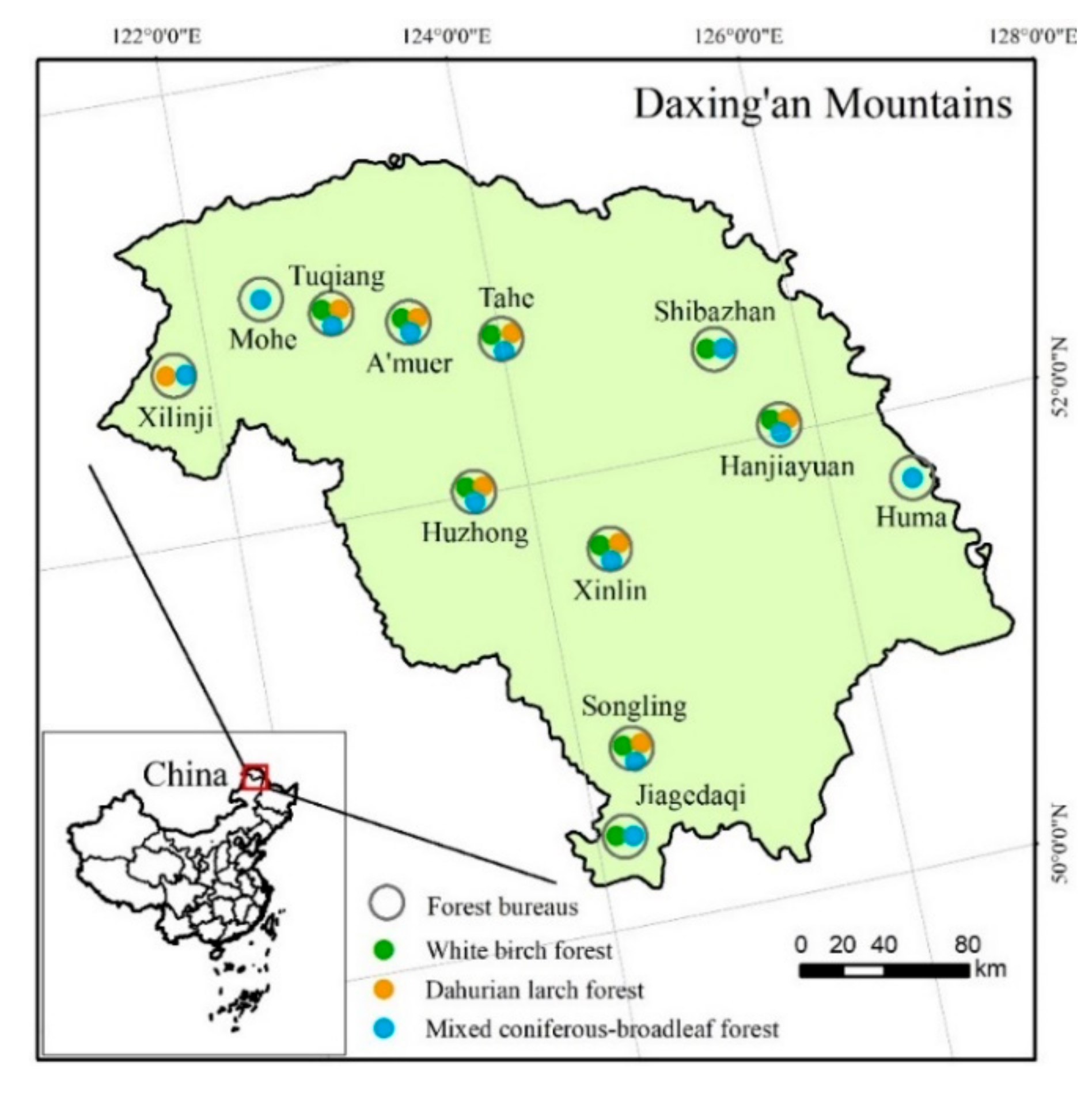
1]. Consequently, China has gradually banned the commercial logging of natural forests in the eastern Daxing’an Mountains since 2015 to recover the natural forests. This ban has been successfully implemented with the current total volume of 547 million m
3 or about 92.01% of the total natural potential of the eastern Daxing’an forest [
2]. However, many natural forests with no production demand need a new management plan to specifically address more appropriate and effective monitoring and adjustment methods to ensure their continuity. One of the most effective ways is to monitor and update real-time forest growth, which significantly impacts forest structure and composition over time [
3]. Unfortunately, to the best of the authors’ knowledge, no research has been found regarding the forest growth model in the eastern Daxing’an Mountains.
Forest growth is defined as the size of a tree or a stand produced within a certain period [
4]. Forest growth and yield research has provided forest managers with an abundance of tools for simulating stand dynamics [
5]. This research was begun in the 1850s in Central Europe when the basic yield tables became the primary standard for growth and yield estimation until the 1950s [
6]. The basic yield tables might be helpful in actual application; however, their low accuracy is gradually becoming unacceptable to both academicians and practitioners. Hence, the mathematical–statistical analysis and modeling of forest growth have been increasingly developed to fulfill the demand for more accurate estimation. As a result, numerous classic functions can be used to better estimate forest growth, such as those of Chapman–Richards, Kangas, Monomolecular, Weibull, and Korf [
7,
8,
9].
However, the growth function is not suitable for the uneven forest, because of the difficulty in determining the age of many natural forests [
10]. Moser and Hall [
11] proposed a function of a measurable size characteristics of the stand under investigation to eliminate the problem of indefinite age. This growth rate equation provides a yield function expressed with an elapsed time from a given initial condition, indicating that compatible growth rate and yield functions for the uneven-aged stand can be derived from permanent plot data. Dale et al. [
12] classified growth and yield models into stand model, size class model, and individual tree model. Peng [
13] detailed the differences between these three models: stand models use stand parameters to simulate the stand growth and yield that are usually simple and robust; however, they provide little or no detail about individual trees within a stand; size class models only require overall stand values as input and provide some information relating to stand structure, but the output is not flexible enough to evaluate a broad range of stand treatments; and the individual tree models simulate each individual tree as a basic unit that provides maximum detail and flexibility for evaluating the stand but requires more detail and an expensive database to be developed and implemented. Although the stand models cannot provide specific information about the individual tree or size class, it is generally cheaper and relatively effective for practical applications because of lesser data and the need for complex variables [
14].
There are several different basic concepts of growth, which have not been properly explained and often appear confusing. Cumulative growth means the total volume attained by a tree or a stand at any particular time. Generally, cumulative growth time is a fixed interval, which is not convenient for practical application. Absolute growth rate (
) is the mean absolute changes in mass over a given time period, which can be defined as the value of a particular characteristic at different times (
and
divided by
).
depends on the current state of the plant size characteristic and is therefore not helpful to growth analysts when comparing plants of different sizes [
15]. In such situations,
is often studied in addition to absolute growth.
is also a function of time and is defined as the increase in size relative to the growth characteristic [
3]. Hunt [
7] decomposed
into the product of three components: (1) the net assimilation rate (
), which is the absolute growth rate per unit leaf area; (2) the leaf mass ratio (
), which is the proportion of biomass invested in leaves; and (3) the specific leaf area (
), which is the leaf area divided by leaf mass. Given the advantages of
in physiology and ecology, it was used in this study as the dependent variable.
Permanent plot data from different regions are mostly used for forest growth modeling. However, heteroscedasticity always exists in model residuals; hence, a weighted regression should be used to neutralize the inconsistency [
16,
17]. The traditional ordinary least-squares (
) method obeys the assumption of independent observations, providing the proper parameter estimates for the overall average. However, their variances are biased when there are significant differences between groups. Since the measured trees or stands are usually grouped into plots or regions, the nonlinear mixed-effects (
) modeling approach has been used to reduce the bias by considering the differences between groups [
18,
19,
20,
21]. The
is composed of fixed- and random-effects parameters, in which the variance–covariance structure analyzes hierarchically structured data more efficiently and subsequently increases the prediction accuracy of the models.
has been widely used in the last few years to describe the response variable, given a set of explanatory variables [
22,
23,
24]. Compared to the conventional
method, quantile regression can characterize the entire conditional distribution of the outcome variable and is more robust to the presence of outliers and misspecification of the error distribution [
25]. However, in actual application, both the
and
should be calibrated for the adjusted random parameters and the best quantile curve [
26,
27,
28].
The main research tasks of this study were to (i) choose the best basic model equation for and solve model autocorrelation and heterogeneity using the and methods; (ii) evaluate different models using a leave-one-out cross-validation approach and compare the of three forest types and analyze the trend differences between mixed and relatively pure stands; and (iii) determine an appropriate sample size that considers both sample cost and predictive accuracy. The finding will be useful in forest management planning for the uneven-aged forests in the eastern Daxing’an Mountains. It will also expand the application of mixed-effects and quantile regression models in stand growth modeling, which will be useful in effectively estimating the dynamics of future forest accumulation and providing a theoretical basis for carbon neutrality. Continuously improving our understanding of impacts on the comparison of pure and mixed forests will support forest managers seeking to develop effective adaptation measures and determine sustainable forestry production.
4. Discussion
In this study, Equation (
25) was the best basic
model constructed using four primary predictors:
,
,
, and
. The data were obtained from the
’s permanent sample plots across the three forest types in eastern Daxing’an Mountains. The exponential form was found to be the best basic
model. Several previous studies have proven that the exponential form can visualize the important biological characteristics of various animal and plant growth. Jobidon [
47] studied the competition effects in the boreal mixed wood forest across Quebec and Canada; he concluded that the exponential form should be considered to analyze the stand growth, specifically if young trees exist. Scolforo et al. [
48] also preferred to utilize the exponential form to model the relative diameter growth rate of the six tree species in Brazil, which included stand density as the primary predictors. The exponential model was proposed in this study since it was able to clearly describe the growth rate of the cold temperate forests and avoid negative growth rate estimation. Most of the native tree species had small
, while only a few individual trees had large
. Hence, these larger trees have smaller predicted growth rate values compared to other trees. The larger trees may highly influence the model; however, the exponential formulation does not allow the predicted growth rate to be negative.
The
was the dependent variable of the model in this paper and was calculated with Pressler’s formula using the average growth rate to replace the consecutive annual growth rate.
is a standard variable to determine the productive capacity of a tree and can be used to compare the trees that differ in initial size, age, and environmental conditions [
49,
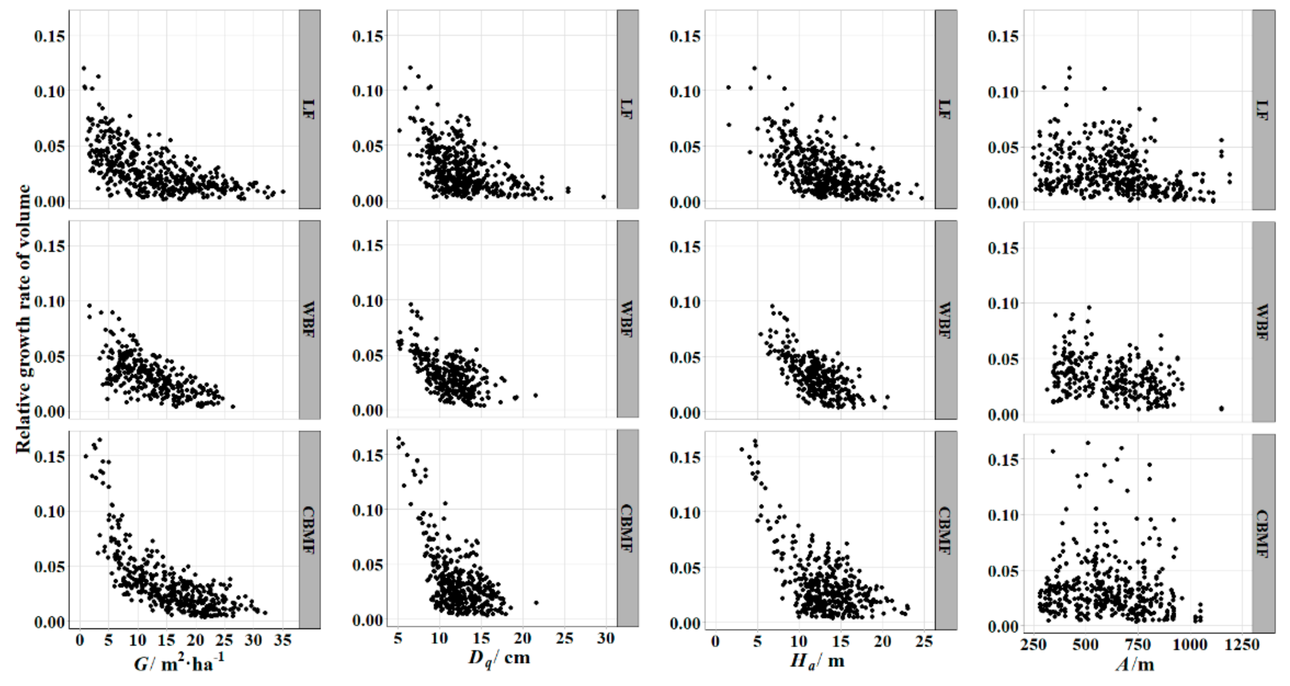
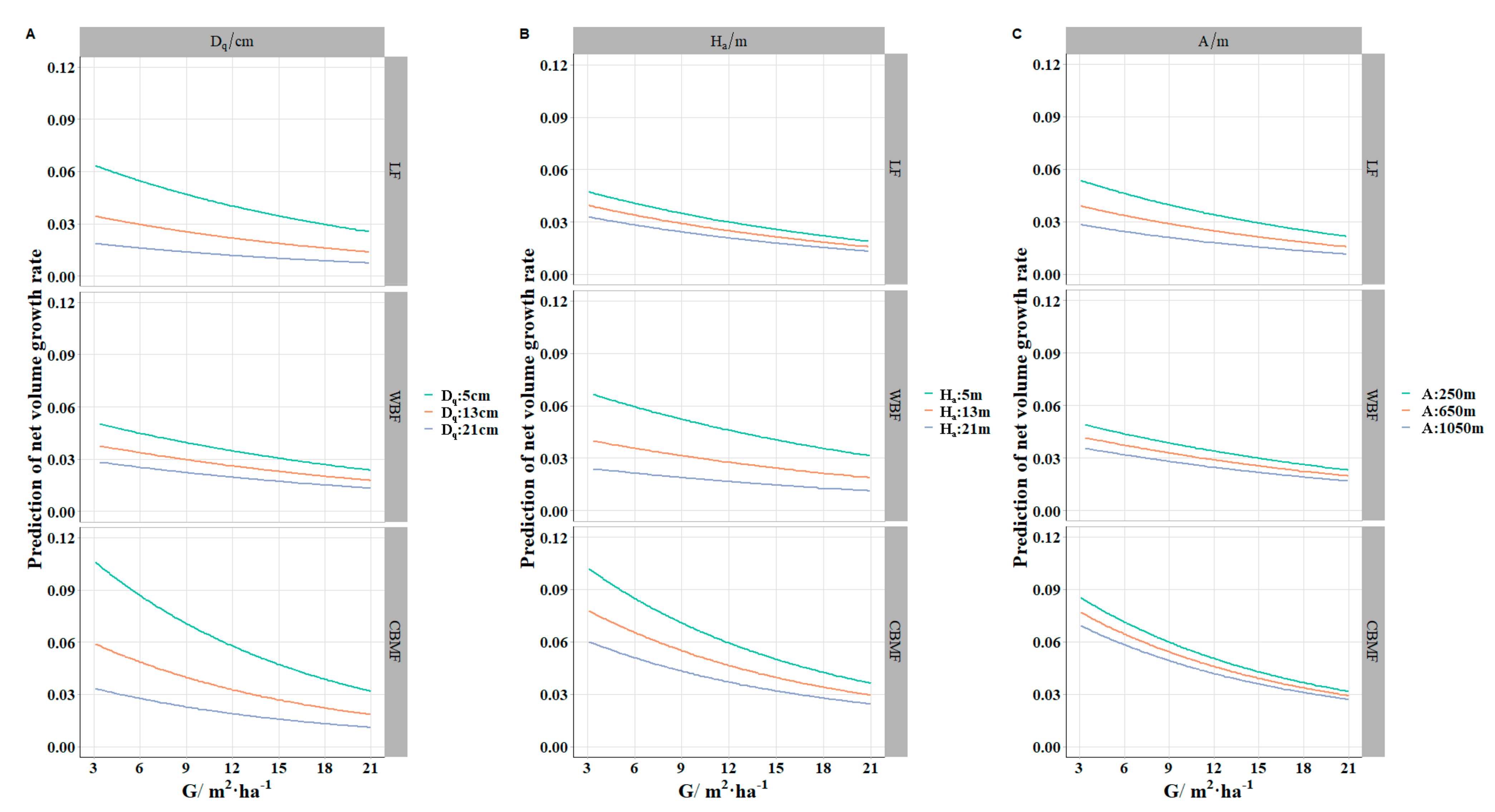
50]. All four parameter estimates were negative, indicating that the
decreased with the increment of various variables. This trend was consistent with the actual survey results (
Figure 2).
was used for the average tree diameter in the research of tree growth, having a better performance than the arithmetic mean diameter [
51,
52]. Curtis et al. [
53] explained the difference between the average and the arithmetic mean diameter in detail and their respective applicable scenarios. Reineke’s [
54]
(stand density index) was used for the various relative density measures and stand management diagrams derived from the Reineke relationship, which was based on
.
was also an important variable for describing stand structure, specifically for the vertical direction.
was the density index, combining the tree diameter and the number of trees within a stand. Site effect variables that contained altitude, slope, and aspect have been recommended in growth, forest species composition, and productivity research [
55,
56,
57]. Unfortunately, in this study, although the altitude showed significant contributions to the
model, the slope and aspect of the plot were not significant in the model. The
declined with altitude, which could be the result of a short growing season and reduction in mean summer temperatures [
58,
59]. Ma and Lei [
60] showed that
can replace dominant height when there is no information available. However, Inoue [
61] found that stand volume and bole surface area were not independent of stand age or site quality. Hence, when the stand age is unknown,
can be the average feedback of stand vertical structure rather than the stand site condition.
The growth of the trees has played an important role in recycling the forest. Plantation forests emerged mainly in Germany and Austria, while the concept of natural forests originated in France and Switzerland [
62]. Although some research on heterogeneous forests was conducted in 1940s, presently, natural forests are still lacking a forest management philosophy. Dahurian larch is a very intolerant and cold-resistant species that can grow in dry, infertile, and swamped soil, or on permanently frozen ground; however, it is best grown in drained, moist, and sandy soil [
63]. Jia and Zhou [
64] summarized the growth characteristics of natural and planted Dahurian larch in Northeast China. They emphasized that the growth rates are considered essential indexes in assessing forest recovery processes and carbon sequestration potentials, which can supply post-fire or sustainable management strategies. White birch is an excellent, fast-growing pioneer species and suitable for well-drained soil; it can grow in heavy clay and nutritionally poor soils [
65]. In recent years, research on the mixed forest has developed rapidly, including stand stability [
66], stand resource utilization [
67], stand diversity [
68], and stand dynamic change [
69]. It has shown that the mixed forest has obvious advantages over the pure forest. The
studied in this paper mainly involved the mixed forest of
and
.
Figure 5 shows that the
of
was higher than
and
across different levels, which proved that
had more potential growth superiority compared with
and
.
also has the highest productivity or stand stability, which was corroborated by the well-known competitive yield criterion [
70].
In forestry applications, two or more measurements are often taken from each sampling unit. These repeated measurements are not statistically independent; hence, the ordinary least-squares techniques may underestimate the variance of parameters. In this paper, the nonlinear mixed model and quantile model were used to deal with the longitudinal data. According to
Table 3, the prediction accuracy of all
models was improved and presented a more stable estimate (indicating the reduction of spatial heterogeneity in the model residuals).
had the most significant improvement, which was then followed by
and
.
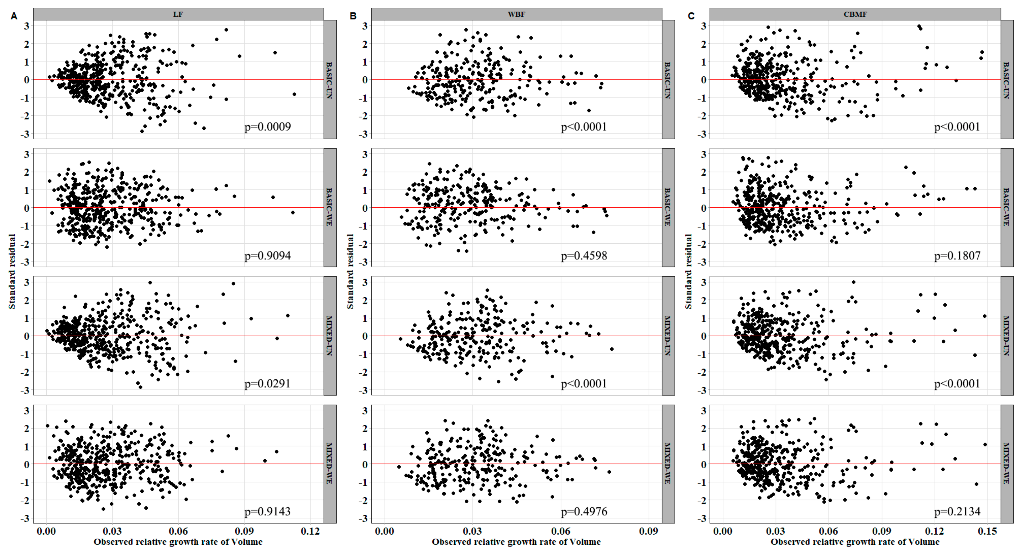
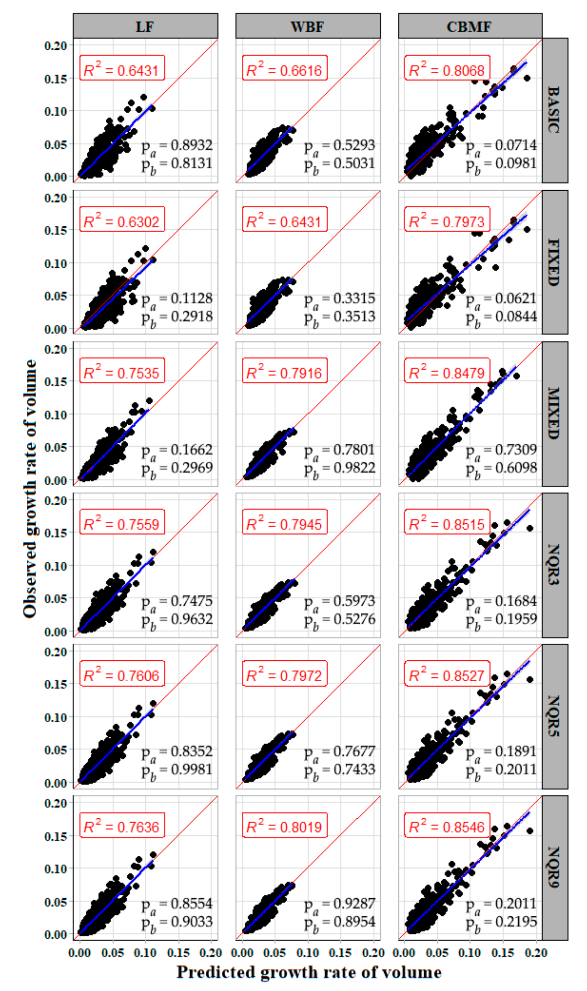
Figure 6 shows that the relationship between the observed value and the predicted value of the mixed model was more concentrated compared with the basic model. The random effect was integrated to
and
for the
mixed model, while
and
were used for
and
, corroborating the results of Condés and García-Robredo [
71]. Zhao et al. [
72] reported that modeling the autocorrelation structure alone cannot completely match the possible common effects, and they suggested introducing random period effects for describing the autocorrelation. Unfortunately, their research relied only on one to three observations; hence, it is unreliable to employ period as an autocorrelation structure.
Cade and Noon [
73] mentioned that the quantile regression estimates multiple rates of change (slopes) from the minimum to maximum response, providing a more complete trend of the variables relationships.
Table 4 shows that the result of the quantile regression model was better than the basic and
models.
and
indicated that more improvement in model accuracy existed for the quantile regression than for the
models.
was a better quantile regression than the others (
and
), although the difference was negligible. Bohora and Cao [
26] showed that
was better than
and
, while Zang et al. [
24] argued that
was the best and used it to model the height–diameter relationship. This kind of contradictory result may be caused by the size and the distribution of the data. The higher quantiles require a much greater proportional increase in data volume to maintain a constant risk ratio, and the excessive numbers of the quantile may cause over-fitting. Therefore, we recommend choosing
or
when the data distribution range is narrow or when the size of the data is limited. In this study, the quantile model had a better result than the
, which was indicated by smaller
,
, and
. The reason might be the obvious differences in growth rate trends between different regions.
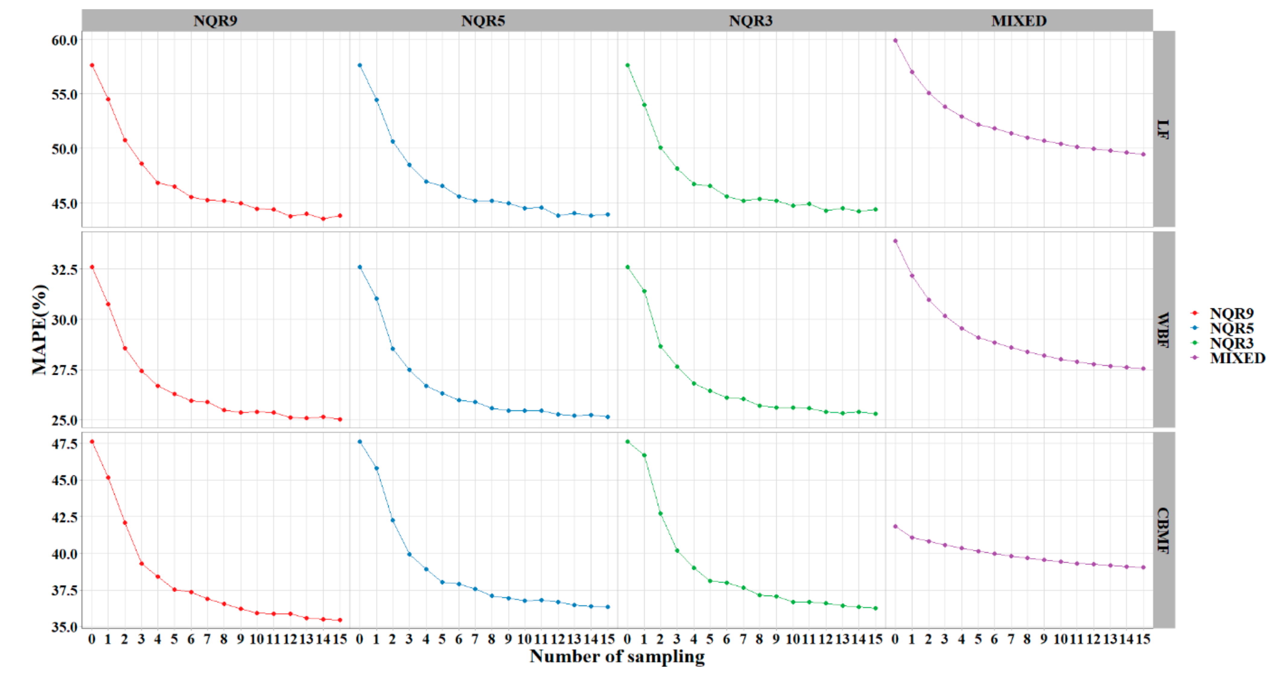
Random sampling was used to calibrate the mixed-effects and quantile models. The results showed that the model performance improved with an increase in the sampling number. The quantile model performed better than the mixed model across all sample numbers, and NQR9 was best among them. Six (or more) sample plots per region were adequate for delivering high-accuracy predictions (
Figure 7,
Table 5). In the mixed-effects or the quantile regression model, the subject-specific random effect or entire conditional distribution of the response makes up the shortcomings of instability and uncertainty of the population-averaged response. The sampling process is a hypothetical simulation of the survey in reality. It can provide prior information to adjust the random parameters or interpolation ratio of the local best quantile curve and effectively improve the accuracy of estimation. It has generally been taken for granted that the inclusion of additional stand variables into the base models automatically results in better predictions (helping to justify the increased costs associated with measuring the additional variables). As Huang et al. [
74] stated, the subject-specific model allows the plot level variations related to many known and unknown factors such as topography, soil type, nutrient status, genetics, climate, silvicultural regime, environment, intra- and inter-specific competitions, etc., to be accounted for without requiring that they be identified or measured. This is a noted advantage of the
and
techniques. In this study, each region contained an average of 32 plots. Assuming the data from the last period are known, the next period
of all plots can be estimated when only six plots from each region are surveyed. This can save about 80% of costs.
5. Conclusions
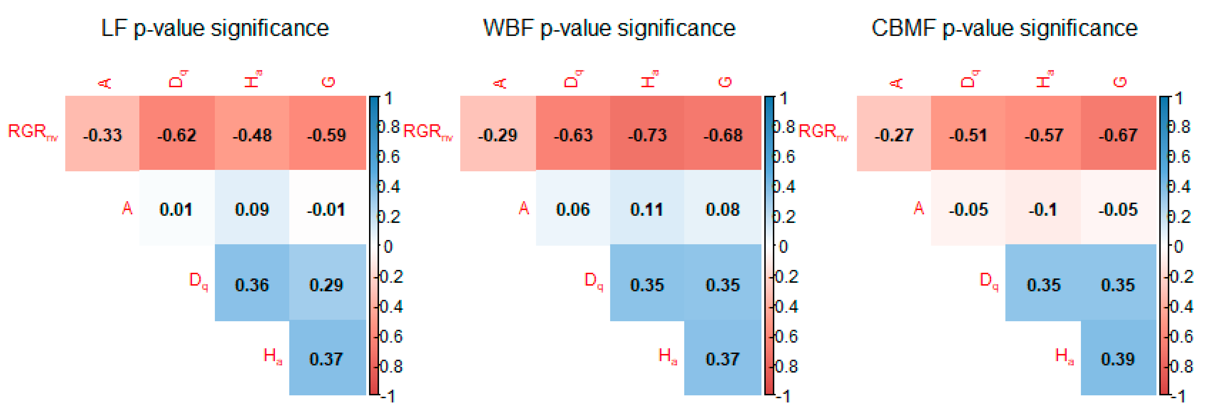
Plantation forests have developed rapidly in modern forestry because of their simple structure, short management cycle, and high timber output. However, there is still a lack of a theoretical basis for natural pure forests and mixed forests. Hence, in this study three forest types from Daxing’an Mountains were studied to determine the growth differences between the natural pure forest and mixed forest and establish the model. was recalculated with the Pressler growth rate formula. The liner model, reciprocal model, power model, exponential model, and sigmoid model were used to develop the basic model, and of these, the exponential model performed the best. The best basic model was established using , , , and surveyed from three periods, using data from 12 forest bureaus in the eastern Daxing’an Mountains, Northeast China, for a total of 1152 samples. A correlation index plot showed that there was no obvious strong relationship between the independent variables. The exponential model was proposed in this study since it was able to clearly describe the growth rate of the cold temperate forests and avoid negative growth rate estimation. All four parameter estimates were negative, indicating that decreased with an increment in various variables. This trend was consistent with the actual survey results. The result showed that the trend of differed among the three forest types, in which had higher than both and , indicating the superiority of mixed forest.
In this paper, four different methods, i.e., , , , and were used to deal with the longitudinal data. All models were validated using the leave-one-out method and random sampling technique. Both quantile regression and methods showed better performance than the basic model. After the addition of random effects, the improved: 0.6841 to 0.7706 (), 0.6990 to 0.7978 (), and 0.8031 to 0.8546 (). outperformed all methods evaluated in this study and provided the best , , and values. Model weighting effectively removed the heteroscedasticity effect of the basic and mixed models. Performance of the methods improved as the sample size increased. Six (or more) sample plots was the most appropriate number and is recommended for model calibration when both prediction accuracy and sampling cost are considered.


