Natural and Human-Transformed Vegetation and Landscape Reflected by Modern Pollen Data in the Boreonemoral Zone of Northeastern Europe

 , and
, and
Abstract
:1. Introduction
2. Materials and Methods
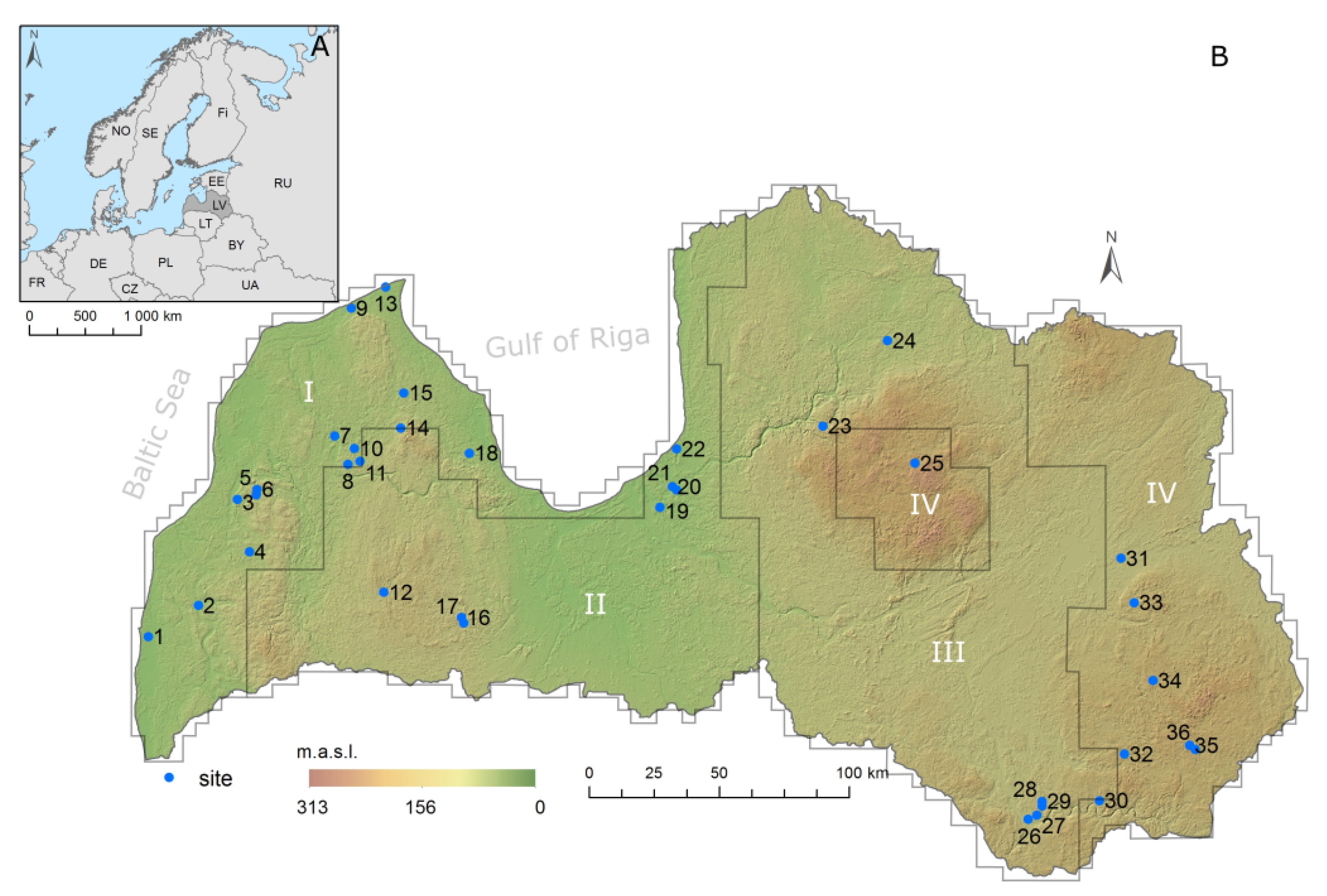
2.1. Study Sites
2.2. Sediment Sampling
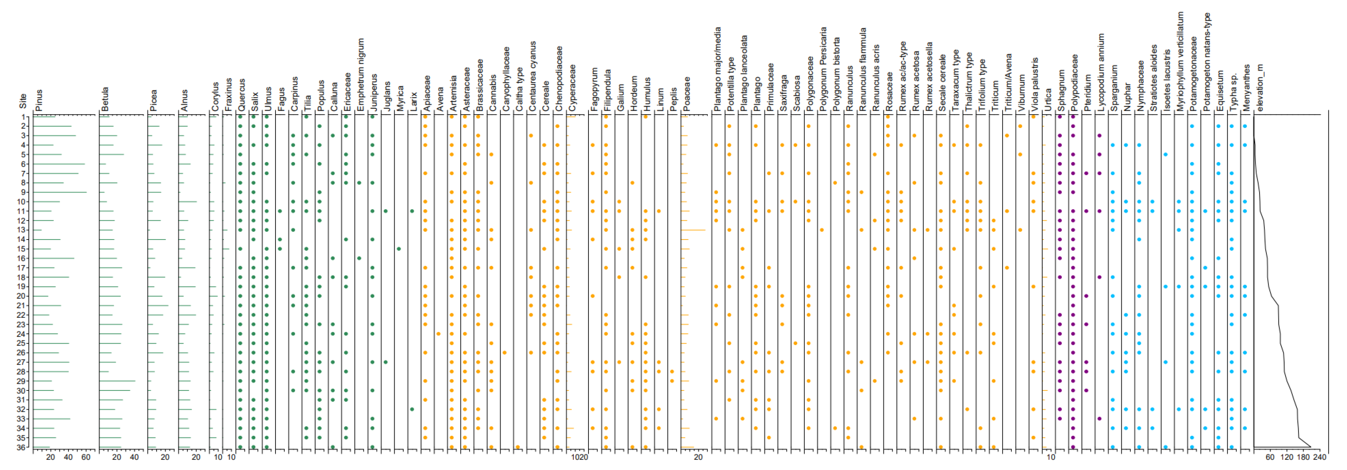
2.3. Pollen Analysis
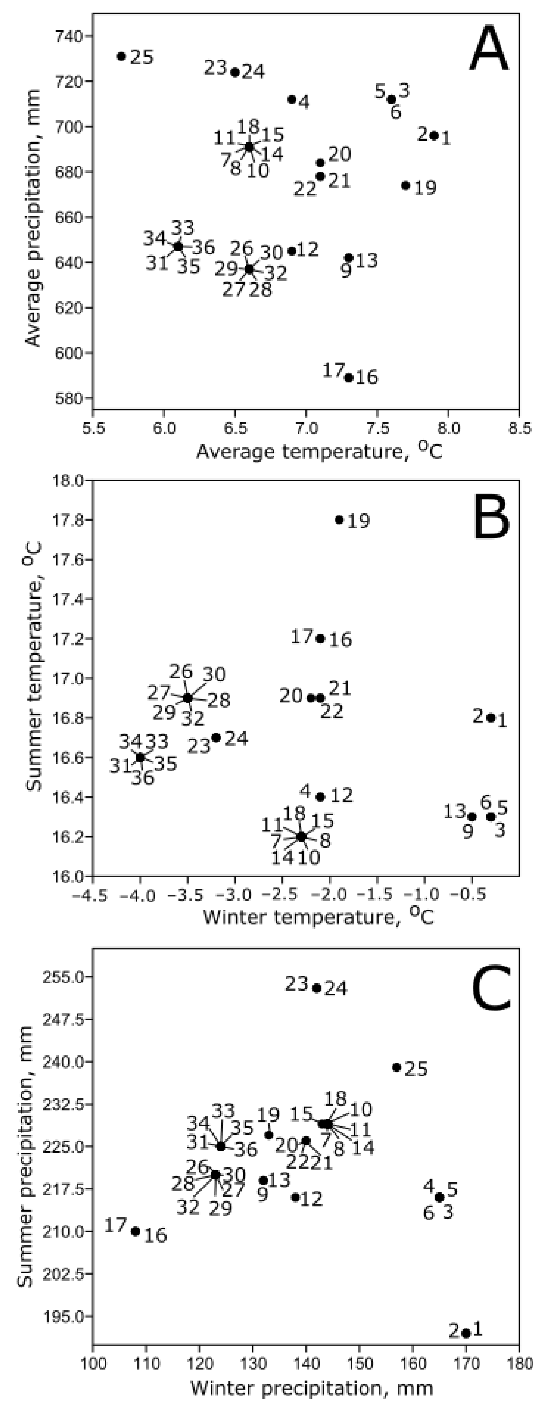
2.4. Climate and Landscape
2.5. Data Analyses
3. Results
3.1. Climate
3.2. Quaternary Sediment and Soil
3.3. Pollen
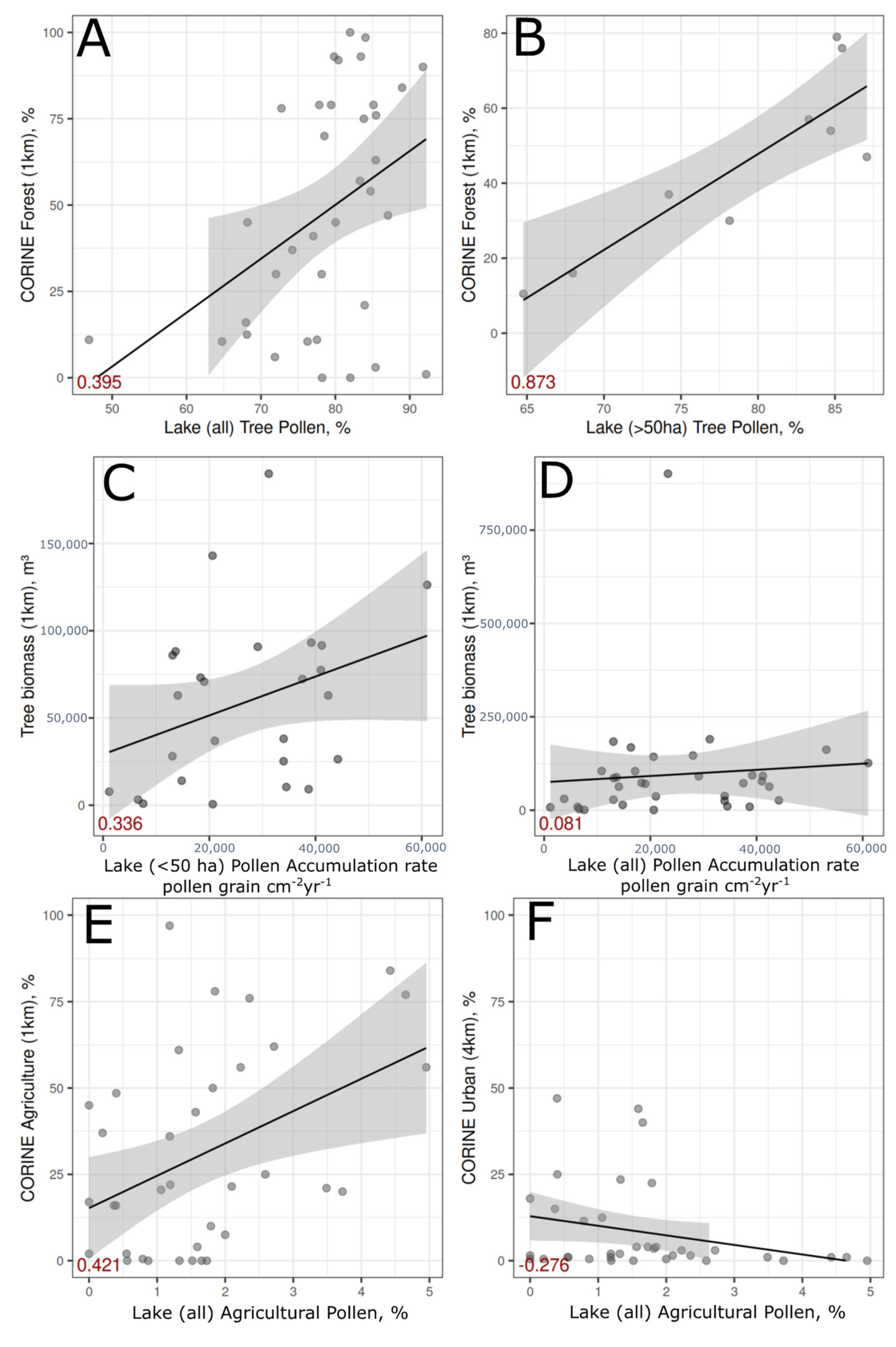
4. Discussion
5. Conclusions
- (1)
- Large waterbodies reflect forest cover better than small-medium-sized waterbodies.
- (2)
- Pollen accumulation rate can be used for forest biomass reconstructions after additional site selection and calibration work.
- (3)
- Agricultural pollen percentages decrease with the increasing urban area around the waterbody.
- (4)
- Modern pollen from surface samples in waterbodies represent current forest and human land use.
- (5)
- Quaternary sediment and subsequent soil type have the main controlling factor for vegetation distribution patterns.
- (6)
- More fertile soils in regions dominated by glacigenic Quaternary sediment show distinct human impact through increased agricultural activities and open landscape.
Supplementary Materials
Author Contributions
Funding
Data Availability Statement
Conflicts of Interest
References
- Sugita, S. Pollen representation of vegetation in Quaternary sediments: Theory and method in patchy vegetation. J. Ecol. 1994, 82, 881–897. [Google Scholar] [CrossRef]
- Sugita, S. Theory of quantitative reconstruction of vegetation. I. Pollen from large sites REVEALS regional vegetation composition. Holocene 2007, 17, 229–241. [Google Scholar] [CrossRef]
- Lisitsyna, O.; Hicks, S.; Huusko, A. Do moss samples, pollen traps and modern lake sediments all collect pollen in the same way? A comparison from the forest limit area of northernmost Europe. Veget. Hist. Archaeobot. 2012, 21, 187–199. [Google Scholar] [CrossRef]
- Seppä, H.; Alenius, T.; Muukkonen, P.; Giesecke, T.; Miller, P.A.; Ojala, A.E.K. Calibrated pollen accumulation rates as a basis for quantitative tree biomass reconstructions. Holocene 2009, 19, 209–220. [Google Scholar] [CrossRef]
- Maguire, K.C.; Nieto-Lugilde, D.; Firzpatrick, M.C.; Williams, J.W.; Blois, J.L. Modeling species and community responses to past, present, and future episodes of climatic and ecological change. Annu. Rev. Ecol. Evol. Syst. 2015, 46, 343–368. [Google Scholar] [CrossRef] [Green Version]
- Reitalu, T.; Gerhold, P.; Poska, A.; Pärtel, M.; Väli, V.; Veski, S. Novel insights into post-glacial vegetation change: Functional and phylogenetic diversity in pollen records. J. Veg. Sci. 2015, 26, 911–922. [Google Scholar] [CrossRef]
- Carvalho, F.; Brown, K.A.; Waller, M.P.; Bunting, M.J.; Boom, A.; Leng, M.J. A method for reconstructing temporal changes in vegetation functional trait composition using Holocene pollen assemblages. PLoS ONE 2019, 14, 1–18. [Google Scholar] [CrossRef]
- Salonen, J.S.; Korpela, M.; Williams, J.W.; Luoto, M. Machine-learning based reconstructions of primary and secondary climate variables from North American and European fossil pollen data. Sci. Rep. 2019, 9, 1–13. [Google Scholar] [CrossRef] [PubMed]
- Tierney, J.E.; Zhu, J.; King, K.; Malevich, S.B.; Hakim, G.J.; Poulsen, C.J. Glacial cooling and climate sensitivity revisited. Nature 2020, 584, 569–573. [Google Scholar] [CrossRef]
- Breitenbach, S.F.M.; Rehfeld, K.; Goswami, B.; Baldini, J.U.L.; Ridley, H.E.; Kennett, D.J.; Prufer, K.M.; Aquino, V.V.; Asmerom, Y.; Polyak, V.J.; et al. Constructing proxy records from age models (COPRA). Clim. Past 2012, 8, 1765–1779. [Google Scholar] [CrossRef] [Green Version]
- Luoto, T.P.; Ojala, A.E.K.; Arppe, L.; Brooks, S.J.; Kurki, E.; Oksman, M.; Wooller, M.J.; Zajaczkowski, M. Synchronized proxy-based temperature reconstructions reveal mid- to late Holocene climate oscillations in High Arctic Svalbard. J. Quat. Sci. 2018, 33, 93–99. [Google Scholar] [CrossRef]
- Reschke, M.; Kröner, I.; Laepple, T. Testing the consistency of Holocene and Last Glacial Maximum spatial correlations in temperature proxy records. J. Quat. Sci. 2021, 36, 20–28. [Google Scholar] [CrossRef]
- IPCC. Climate Change 2014: Synthesis Report. In Core Writing Team, Contribution of Working Groups I, II and III to the Fifth Assessment Report of the Intergovernmental Panel on Climate Change; Pachauri, R.K., Meyer, L.A., Eds.; IPCC: Geneva, Switzerland, 2014; p. 151. [Google Scholar]
- Davis, B.A.S.; Chevalier, M.; Sommer, P.; Carter, V.A.; Finsinger, W.; Mauri, A.; Phelps, L.N.; Zanon, M.; Abegglen, R.; Ǻkesson, C.M.; et al. The Eurasian Modern Pollen Database (EMPD), Version 2. Earth Syst. Sci. Data 2020, 12, 2423–2445. [Google Scholar] [CrossRef]
- Zawiska, I.; Dimante-Deimantovica, I.; Luoto, T.P.; Rzodkiewicz, M.; Saarni, S.; Stivrins, N.; Tylmann, W.; Lanka, A.; Robeznieks, M.; Jilbert, T. Long-term consequences of water punping on the ecosystem functioning of Lake Sekšu, Latvia. Water 2020, 12, 1459. [Google Scholar] [CrossRef]
- Stivrins, N.; Grudzinska, I.; Elmi, K.; Heinsalu, A.; Veski, S. Determining reference conditions of hemiboreal lakes in Latvia, NE Europe: A palaeolimnological approach. Ann. Limnol. Int. J. Limnol. 2018, 54, 1–22. [Google Scholar] [CrossRef]
- Laiviņš, M.; Melecis, V. Bio-geographical interpretation of climate data in Latvia: Multidimensional analysis. Acta Uni. Latv. 2003, 654, 7–22. [Google Scholar]
- Berglund, B.E.; Ralska-Jasiewiczowa, M. Pollen analysis and pollen diagrams. In Handbook of Holocene Palaeoecology and Palaeohydrology; Berglund, B.E., Ed.; Wiley: Chichester, UK, 1986; pp. 455–484. [Google Scholar]
- Stockmarr, J. Tablets with spores used in absolute pollen analysis. Pollen Spore 1971, 13, 615–621. [Google Scholar]
- Moore, P.D.; Webb, J.A.; Collinson, M.E. Pollen Analysis; Blackwell Scientific Publications: Oxford, UK, 1991; p. 216. [Google Scholar]
- Grimm, E.C. Tilia Software for Palynologists. 2021. Available online: www.tiliait.com (accessed on 14 June 2019).
- European Environmental Agency. Corine Land Cover Data; European Union, Copernicus Land Monitoring Service: 2020. Available online: https://land.copernicus.eu/pan-european/corine-land-cover/clc2018 (accessed on 20 April 2021).
- State Forest Service. State Forest Register Database; State Forest Service: Riga, Latvia, 2019. Available online: https://latvija.lv/en/PPK/uznemejdarbiba/registri/p6431/ProcesaApraksts (accessed on 5 July 2020).
- Geological Map of Latvia. Quaternary Deposits; Scale 1:200,000; State Geological Survey: Riga, Latvia, 1997.
- Matthias, I.; Giesecke, T. Insights into pollen source area, transport and deposition from modern pollen accumulation rates in lake sediments. Quat. Sci. Rev. 2014, 87, 12–23. [Google Scholar] [CrossRef]
- Davis, J.C. Statistics and Data Analysis in Geology; John Wiley and Sons: Hoboken, NJ, USA, 1986; p. 140. [Google Scholar]
- Legendre, P.; Legendre, L. Numerical Ecology, 2nd ed.; Elsevier: Amsterdam, The Netherlands, 1998; p. 853. [Google Scholar]
- Jackson, D.A. Stopping rules in principal components analysis: A comparison of heuristical and statistical approaches. Ecology 1993, 74, 2204–2214. [Google Scholar] [CrossRef]
- Hammer, Ø.; Harper, D.A.T.; Ryan, P.D. PAST: Paleontological statistics software package for education and data analysis. Palaeontol. Electron. 2001, 4, 9. [Google Scholar]
- R Core Team. R: A Language and Environment for Statistical Computing; R Foundation for Statistical Computing: Vienna, Austria, 2021; Available online: https://www.R-project.org/ (accessed on 22 February 2021).
- Seppä, H.; Birks, H.J.B.; Odland, A.; Poska, A.; Veski, S. A modern pollen-climate calibration set from northern Europe: Developing and testing a tool for palaeoclimatological reconstructions. J. Biogeogr. 2004, 31, 251–267. [Google Scholar] [CrossRef]
- Forest Statistics in Latvia. Meža Statistikas CD (vmd.gov.lv). 2018. Available online: https://www.vmd.gov.lv/valsts-meza-dienests/statiskas-lapas/publikacijas-un-parskati/meza-statistikas-cd?nid=1809#jump (accessed on 4 April 2021).
- Poska, A.; Saarse, L.; Koppel, K.; Nielsen, A.B.; Avel, E.; Vassiljev, J.; Vali, V. The Varijärv area, South Estonia over the last millennium: A high resolution quantitative land-cover reconstruction based on pollen and historical data. Rev. Palaeobot. Palynol. 2014, 207, 5–17. [Google Scholar] [CrossRef]
- Sugita, S. Theory of quantitative reconstruction of vegetation. II. All you need is LOVE. Holocene 2007, 17, 243–257. [Google Scholar] [CrossRef]
- Prentice, I.C. Records of vegetation in time and space: The principles of pollen analysis. In Vegetation History; Huntley, B., Webb, T., Eds.; Kluwer Academic Publishers: Dordrecht, The Netherlands, 1988; pp. 17–42. [Google Scholar]
- Poska, A.; Meltsov, V.; Sugita, S.; Vassiljev, J. Relative pollen productivity estimates of major anemophilous taxa and relevant source area of pollen in a cultural landscape of the hemi-boreal forest zone (Estonia). Rev. Palaeobot. Palynol. 2011, 167, 30–39. [Google Scholar] [CrossRef]
- Theuerkauf, M.; Drager, N.; Kienel, U.; Kuparinen, A.; Brauer, A. Effects of changes in land management practices on pollen productivity of open vegetation during the last century derived from varved lake sediments. Holocene 2015, 25, 733–744. [Google Scholar] [CrossRef]
- Chevalier, M.; Davis, A.S.; Heiri, O.; Seppä, H.; Chase, B.M.; Gajewski, K.; Lacourse, T.; Telford, R.J.; Finsinger, W.; Guiot, J.; et al. Pollen-based climate reconstruction techniques for late Quaternary studies. Earth-Sci. Rev. 2020, 210, 103384. [Google Scholar] [CrossRef]


| No | Site Name | Coordinates, N, E | Elevation, m a.s.l. | Size, ha | Water Depth, max/mean, m | Hydrology, Throughflow/Inflow/Outflow/None | Reference |
|---|---|---|---|---|---|---|---|
| 1 | Lake Liepājas | 56°29′21.35″ 21°2′58.65″ | 0.2 | 3715 | 2.8/2 | throughflow | This study |
| 2 | Lake Durbes | 56°36′40.91″ 21°21′1.05″ | 23 | 670 | 8.1/3.9 | throughflow | This study |
| 3 | Dam Alsungas | 56°58′50.82″ 21°34′19.07″ | 22 | 7.8 | 2.5/2 | throughflow | This study |
| 4 | Lake Ķikuru | 56°48′4.45″ 21°39′38.57″ | 38.7 | 21.6 | 4.3/1.9 | throughflow | [14] |
| 5 | Lake Pinku | 56°59′56.82″ 21°41′17.77″ | 54 | 29 | 20/5 | throughflow | This study |
| 6 | Pond Cūku | 57°1′2.44″ 21°41′36.71″ | 42.5 | 1.2 | 1.2/0.6 | throughflow | This study |
| 7 | Lake Usmas | 57°11′52.23″ 22°7′50.94″ | 21 | 3469.2 | 17/5.4 | throughflow | This study |
| 8 | Lake Sūnezers | 57°6′46.93″ 22°15′55.74″ | 48.8 | 1.4 | 3.7/1.5 | none | [14] |
| 9 | Lake Lielais Pēterezers | 57°39′13.93″ 22°15′39.45″ | 9 | 2.9 | 3.1/2 | none | This study |
| 10 | Lake Rūmiķis | 57°10′8.37″ 22°18′12.79″ | 40 | 1.5 | 4.3/1.5 | outflow | [14] |
| 11 | Lake Vēžezers | 57°7′28.75″ 22°20′26.79″ | 50 | 7 | 1.7/1.4 | outflow | [14] |
| 12 | Lake Saldus | 56°40′26.92″ 22°30′39.42″ | 89 | 22 | 4.6/2.5 | throughflow | This study |
| 13 | Dam Vaides | 57°43′42.71″ 22°28′35.54″ | 6.2 | 5.4 | 1.7/1 | throughflow | This study |
| 14 | Lake Talsu | 57°14′33.58″ 22°35′47.27″ | 64 | 3.6 | 16.5/11.6 | throughflow | This study |
| 15 | Lake Sasmakas | 57°21′55.39″ 22°36′36.21″ | 36 | 252 | 7.4/3.8 | throughflow | This study |
| 16 | Lake Sesavas lake | 56°34′18.38″ 23°1′1.67″ | 36.6 | 17 | 4.2/2.7 | throughflow | This study |
| 17 | Lielais Vipēdes | 56°35′28.07″ 23°0′2.33″ | 96 | 20.1 | 3.3/2.3 | throughflow | This study |
| 18 | Lake Vaskaris | 57°9′35.68″ 23°2′11.71″ | 15.4 | 22.1 | 2.8/1 | throughflow | [14] |
| 19 | Lake Velnezers | 56°58′34.47″ 24°14′48.84″ | 4.5 | 3.5 | 6/3.5 | none | This study |
| 20 | Lake Sekšu | 57°2′12.33″ 24°21′8.38″ | 5 | 11.7 | 6/2.5 | inflow | [14] |
| 21 | Lake Mazais Baltezers | 57°2′50.15″ 24°19′42.49″ | 0.2 | 198.7 | 10.3/4.6 | throughflow | This study |
| 22 | Lake Lilastes | 57°10′52.30″ 24°21′25.42″ | 0.5 | 183.6 | 3.2/2 | throughflow | This study |
| 23 | Lake Āraišu | 57°15′1.02″ 25°17′24.02″ | 120.2 | 32.6 | 12.2/4 | throughflow | [14] |
| 24 | Lake Trikātas | 57°32′28.40″ 25°42′52.31″ | 50 | 13 | 6.5/1.8 | throughflow | [14] |
| 25 | Lake Bricu | 57°6′55.06″ 25°52′15.45″ | 207.3 | 16 | 2.7/1.3 | throughflow | [14] |
| 26 | Pond Esplanādes | 55°52′18.51″ 26°30′23.69″ | 89.4 | 1.5 | 3.2/2 | none | This study |
| 27 | Lake Gubiščes | 55°53′3.92″ 26°33′43.89″ | 108 | 18.5 | 2/1 | none | This study |
| 28 | Lake Mazais Stropu | 55°54′41.96″ 26°35′29.00″ | 110.8 | 15.3 | 4.3/2.7 | outflow | This study |
| 29 | Lake Lielais Stropu | 55°54′41.96″ 26°35′29.00″ | 110 | 417.9 | 6.3/3.6 | throughflow | This study |
| 30 | Lake Gluhoje | 55°55′34.64″ 26°57′2.54″ | 13.5 | 1.7 | 3.5/1.9 | none | This study |
| 31 | Lake Lielais Svētiņu | 56°45′38.20″ 27°8′57.84″ | 96.2 | 18.8 | 5.8/2.9 | throughflow | [14] |
| 32 | Lake Čertoks | 56°5′1.88″ 27°6′59.13″ | 159 | 1.9 | 18.3/16 | none | This study |
| 33 | Lake Puderovas | 56°36′19.19″ 27°13′17.91″ | 145.9 | 9.7 | 4.5/1.5 | throughflow | This study |
| 34 | Lake Zosnas | 56°20′3.09″ 27°18′49.65″ | 163.5 | 156.5 | 15.4/6 | throughflow | This study |
| 35 | Lake Dagdas | 56°5′13.72″ 27°33′30.01″ | 158.1 | 484.1 | 19.2/5.2 | throughflow | This study |
| 36 | Pond Dagdas | 56°6′11.33″ 27°31′19.50″ | 162 | 0.33 | 2.4/1.2 | none | This study |
| Continentality Index | Air Temperature, °C | Maximal Freezing of Soil, cm | Snow Coverage, Days | Maximal Water Content in Snow, mm | Elevation, m a.s.l. | Distance to Sea, km | |||
|---|---|---|---|---|---|---|---|---|---|
| January | Annual | Absolute Minimum | Annual Minimum | ||||||
| Weak | −3.7 | 5.8 | −33.6 | −22.2 | 38.4 | 87 | 39 | 32 | 13 |
| Moderate | −5.2 | 5.5 | −35.5 | −25.5 | 44.8 | 97 | 49 | 54 | 46 |
| Average | −6.6 | 5.1 | −39.6 | −27.8 | 53.7 | 114 | 71 | 98 | 109 |
| Strong | −7.4 | 4.9 | −40.5 | −29.2 | 57.8 | 123 | 89 | 154 | 186 |
Publisher’s Note: MDPI stays neutral with regard to jurisdictional claims in published maps and institutional affiliations. |
© 2021 by the authors. Licensee MDPI, Basel, Switzerland. This article is an open access article distributed under the terms and conditions of the Creative Commons Attribution (CC BY) license (https://creativecommons.org/licenses/by/4.0/).
Share and Cite
Stivrins, N.; Briede, A.; Steinberga, D.; Jasiunas, N.; Jeskins, J.; Kalnina, L.; Maksims, A.; Rendenieks, Z.; Trasune, L. Natural and Human-Transformed Vegetation and Landscape Reflected by Modern Pollen Data in the Boreonemoral Zone of Northeastern Europe. Forests 2021, 12, 1166. https://doi.org/10.3390/f12091166
Stivrins N, Briede A, Steinberga D, Jasiunas N, Jeskins J, Kalnina L, Maksims A, Rendenieks Z, Trasune L. Natural and Human-Transformed Vegetation and Landscape Reflected by Modern Pollen Data in the Boreonemoral Zone of Northeastern Europe. Forests. 2021; 12(9):1166. https://doi.org/10.3390/f12091166
Chicago/Turabian StyleStivrins, Normunds, Agrita Briede, Dace Steinberga, Nauris Jasiunas, Jurijs Jeskins, Laimdota Kalnina, Alekss Maksims, Zigmars Rendenieks, and Liva Trasune. 2021. "Natural and Human-Transformed Vegetation and Landscape Reflected by Modern Pollen Data in the Boreonemoral Zone of Northeastern Europe" Forests 12, no. 9: 1166. https://doi.org/10.3390/f12091166
APA StyleStivrins, N., Briede, A., Steinberga, D., Jasiunas, N., Jeskins, J., Kalnina, L., Maksims, A., Rendenieks, Z., & Trasune, L. (2021). Natural and Human-Transformed Vegetation and Landscape Reflected by Modern Pollen Data in the Boreonemoral Zone of Northeastern Europe. Forests, 12(9), 1166. https://doi.org/10.3390/f12091166