New Perspectives for LVL Manufacturing from Wood of Heterogeneous Quality—Part. 1: Veneer Mechanical Grading Based on Online Local Wood Fiber Orientation Measurement

Abstract

The grading of wood veneers according to their true mechanical potential is an important issue in the peeling industry. Unlike in the sawmilling industry, this activity does not currently estimate the local properties of production. The potential of the tracheid effect, which enables local fiber orientation measurement, has been widely documented for sawn products. A measuring instrument exploiting this technology and implemented on a peeling line was developed, enabling us to obtain the fiber orientation locally which, together with global density, allowed us to model the local elastic properties of each veneer. A sorting method using this data was developed and is presented here. It was applied to 286 veneers from several logs of French Douglas fir, and was compared to a widely used sorting method based on veneer appearance defects. The effectiveness of both grading approaches was quantified according to mechanical criteria. This study shows that the sorting method used (based on local fiber orientation and average density) allows for better theorical quality discrimination according to the mechanical potential. This article is the first in a series, with the overall aim of enhancing the use of heterogeneous wood veneers in the manufacturing of maximized-performance LVL by veneer grading and optimized positioning as well as material mechanical property modelization.

1. Introduction

Laminated veneer lumber (LVL) is an engineered wood product made from veneers that is obtained by rotary peeling. It is used in many structural applications such as beams, columns, or panels due to its consistently high mechanical performance and improved dimensional stability in comparison with solid timber [1]. LVL-P is defined in the technical literature as a layup of 3 mm veneers laid in the same direction [1]. As a result, LVL-P is the LVL material that presents the best possible mechanical properties within the grain direction, and thus LVL-P beams are often produced using the highest strength grade of veneers to optimize the beam dimensions and provide good material efficiency. To obtain great dimensional stability relative to humidity conditions, LVL-P elements are usually slender beams with a thickness-to-width ratio of 1:8 at a maximum. They are mainly applied horizontally as flooring supports subjected to edgewise bending or as studs for wall structures [1].

In the peeling industry, the sorting of veneers to differentiate their quality is usually performed according to appearance criteria (knot size, slots, resin pockets, etc.) based on the EN 635-3 standard [2]. This classification is generally undertaken through the use of cameras integrated into the panel-making line. However, these appearance criteria present a low correlation with mechanical properties. Thus, some criteria should to be defined for mechanical sorting purposes. Unlike in the peeling industry, in the sawmilling industry mechanical property assessment using grading machines (stress grading, vibrational tests) based on physical measurements has been developed. In recent scientific advances, two main technologies are used for better timber quality assessment: X-ray scanning, which provides local density through board thickness, and laser-dot scanning, which provides the local fiber orientation on board surfaces. With wood being a highly anisotropic material, the strength and stiffness properties are far better in the longitudinal fiber direction than in perpendicular. It appears that models based on fiber orientation measurement could provide greater improvements in bending strength prediction as compared to X-ray scanning [3]. This quantitative measurement of wood anisotropy may be the reason why fiber orientation-based models are better than local density (X-ray)-based models, which only indirectly estimate the wood properties from the local density (mainly clear wood density and knots) [4]. However, for species such as Douglas fir that are variable in terms of density and perturbated local fiber orientation, both should be considered.

The assessment of the mechanical potential of veneers by physical measures is therefore important for veneer grading, but the implementation of existing technologies from the sawmill to the peeling line is not simple. The X-ray scanning of veneers on a peeling line is expensive to implement, mainly because of the larger width of the veneers (several meters) as compared to sawn boards (up to 200 mm).

Conversely, laser-dot scanning is easier, cheaper, and safer to implement in a peeling line than X-ray scanning. Laser-dot scanning (also known as fiber-orientation scanning), is based on the light scattering of a laser dot projected on the wood surface, called the “tracheid effect” [5,6,7]. Laser dots on the wood surface scatter in quasi-elliptically shaped light spots according to fiber orientation. These ellipses can be acquired with standard cameras, and then the obtained pictures can be binarized. The contour of the binarized ellipses is fitted to an ellipse equation, and the angle between the major axis of the ellipse and the longitudinal direction of the board is defined. A great advantage of this method is that the measure can be performed on green wood veneers. Indeed, the high moisture content makes the ellipses larger and thus easier to measure with great accuracy, allowing the use of low and safe power lasers [7]. Moreover, green veneers are not subject to drying deformation in the 3D space, allowing for regular measurement in the LT plan. As a result, the in-line assessment device cost is cheaper and the protective fairing can be unfussy.

Much research using this technology has been performed recently: a similar modeling method of the mechanical properties of sawn timber was simultaneously developed by the LaBoMaP [8,9,10] and Linnaeus University of Vaxjö, Sweden [11,12,13]. Viguier et al. [14] successfully adapted this modeling method based on the fiber orientation scanning of small dimensions veneers that were scanned with a laser-dot scanner which usually worked with sawn timber. These authors showed that it was possible to model the flatwise bending stiffness of a LVL-P from the laser-dot scanning of the constituted veneers. Morover, they pointed out the fact that knowledge of the local fiber orientation is particularly important for homogeneous species such as beech. However, no study of the edgewise bending test was performed because of the small dimensions of the samples. Frayssinhes et al. [15] showed the first results of an online laser-dot scanner, the Local Online Orientation fiBer AnalyseR (LOOBAR), which is able to measure local fiber orientation directly during the rotary peeling process, and is thus not limited by the width of a sawmill type laser-dot scanner. These authors proved the ability of the device to measure the local fiber orientation and compared it to a fiber deviation model based on the distribution and size of knots, but no assessment of veneer mechanical properties was made.

The present paper aims to show the possible processing based on local fiber orientation measurements with the LOOBAR device in order to assess the mechanical properties of veneers and grade them in different strength classes. This article will first describe the LOOBAR constitution and its inner operations. Then, a method will be proposed that allows classes to be developed using physical parameters, combining the local fiber orientation and the average density. We propose testing the measurement and method on peeling and processing data from a very heterogeneous resource for which sorting is all the more necessary: the French large-diameter Douglas fir. The main objective is to compare this innovative sorting method to the sorting criteria method based on the visual observation of knots (like EN 635-3 standard [2]) at the scale of the veneers, and determine its consequences for LVL-P beams subjected to edgewise bending.

2. Materials and Methods

Table 1. Nomenclature.

List of Main Symbols
$\overline{{\rho }_{veneer}}$	Averaged veneer density at 12% moisture content (kg·m−3)	$E_T$	Sorting threshold in terms of modulus of elasticity (MPa)
$\theta \left(x,y\right)$	Local fiber orientation angle (°)	$\overline{E_{veneer}}$	Averaged local modulus of elasticity on all veneer surfaces (MPa)
$\overline{E_{beam}}\left(x,y\right)$	Average of $E_{ply,n}\left(x,y\right)$ of the 15 constitutive plies (MPa)	$\overline{E_x}\left(x\right)$	Stiffness profile: averaged local modulus of elasticity along the length of the veneer (MPa)
$E_{eq}$	Beam equivalent modulus of elasticity (MPa)	$E_x\left(x,y\right)$	Local modulus of elasticity of the veneer (MPa)
$E{I}_{eff}\left(x\right)$	Effective bending stiffness profile along the length of the beam (N·mm²)	${\overline{E_x}}_{min}$	Stiffness profile minimum value (MPa)
$E{I}_{eff}{}_{min}$	Effective bending stiffness profile minimum value (N·mm²)	$\overline{H_{veneer}}$	Averaged normalized local Hankinson value on all veneer surfaces (dimensionless quantity)
$E_{ply,n}\left(x,y\right)$	Local modulus of elasticity of ply (MPa)	KSR	Knot surface ratio (d.q.)

shows is the nomenclature listing the main symbols used.

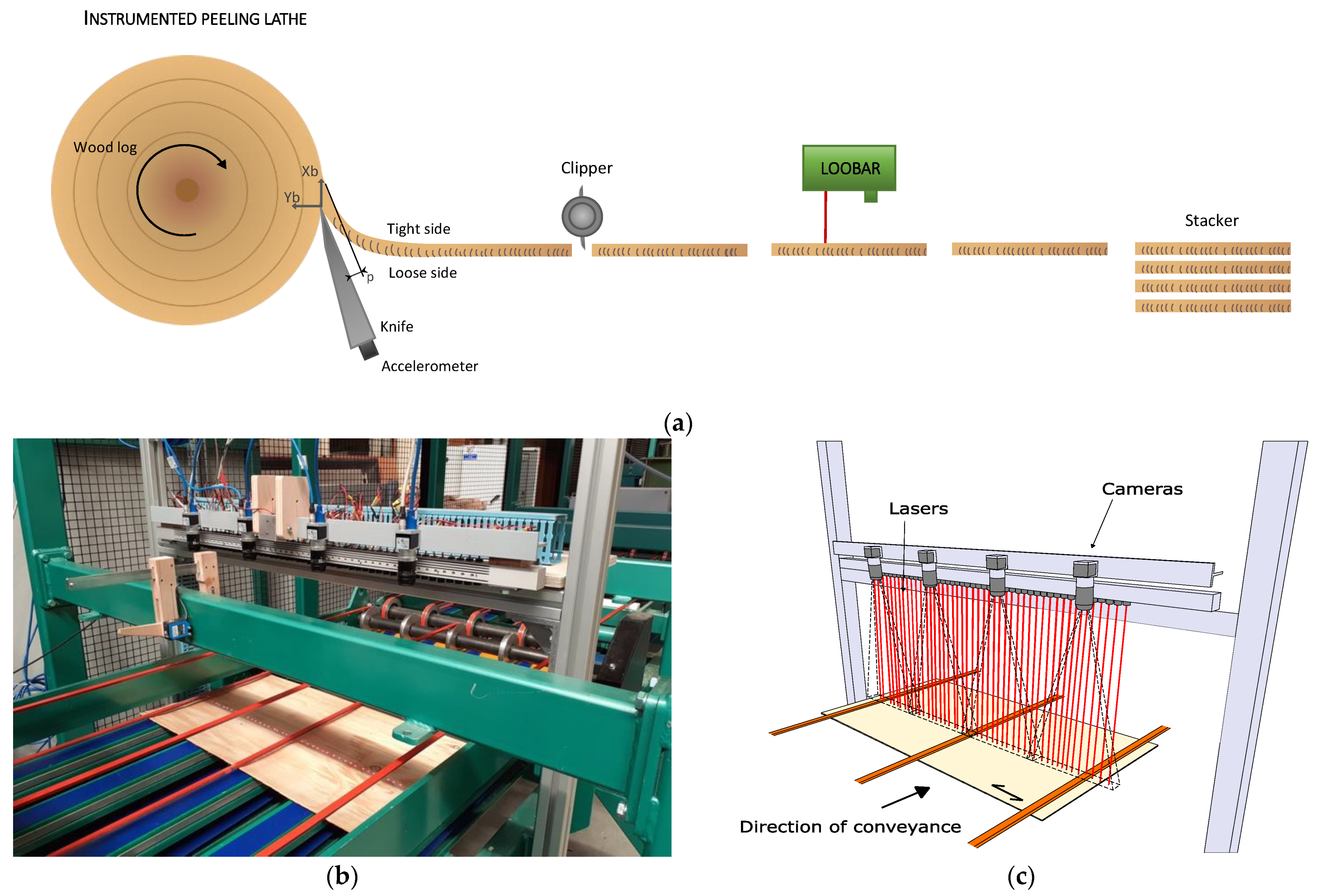
2.1. Douglas-Fir Forest Stand and Peeling

Three different samples compose the Douglas-fir (Pseudotsuga menziesii (Mirb.) Franco) resource used for the experimental peeling/scanning (

Table 2. Forest stands.

	Forest Stand 1	Forest Stand 2	Forest Stand 3
Locality	Sémelay (Nièvre, France)	Anost (Saône-et-Loire, France)	Cluny (Saône-et-Loire, France)
Average altitude	300–400 m	300–400 m	300–400 m
Cutting age	50–60 yo	50–60 yo	50–60 yo
Silviculture	Fourth thinned-out plot, non pruned wood	Clearcut, dynamic sylviculture, pruned wood	Classic (high forest)
Number of logs	4	4	7
Number of veneers	Sapwood: 68 Heartwood: 57	Sapwood: 8 Heartwood: 24	Sapwood: 47 Heartwood: 82
Average under bark trunk diameter	Min: 425 mm Max: 470 mm	Min: 410 mm Max: 445 mm	Min: 420 mm Max: 455 mm
Veneer average density	527 kg·m−3	508 kg·m−3	544 kg·m−3

).

The peeling operation took place using the LaBoMaP rotary peeling machine in Cluny, France. All logs were preliminarily soaked in water at 50 °C before peeling during a minimum of 36 h, intending to ease the rotary peeling by increasing the material deformability [16]. The linear cutting speed was automatically controlled by the machine at 1.5 m·s⁻¹ [17]. The rotary peeling operation was carried out without the use of a pressure bar since the lathe was not equipped with a roller pressure bar. This choice was made to avoid any problems coming from the Horner effect [18]. The peeling thickness was set to obtain dried veneers with a thickness of 3 mm. Scratcher knifes were set up, allowing the incision of the log on the surface prior to the cutting of the knife. This allowed a clean cut of veneer edges perpendicularly to the spindle axe. The distance between scratcher knives was adjusted to a nominal length of between 700 and 750 mm according to the length of each log. Concerning the cutting width of the veneers (perpendicular to the grain), it was adjusted according to the external aspect of the log (visible knottiness, radial cracks). A log that is radially cracked has a greater propensity to form discontinuities in the peeling ribbon. A short trimming length was chosen to maximize the number of uncracked veneers. The 2 chosen widths were 850 mm and 1000 mm. In total, the data coming from 286 veneers were treated in the following studies, coming from the peeling and online scanning of 12 Douglas-fir logs (see Table 2).

Heartwood was manually separated from sapwood through visual sorting based on veneer color. In Douglas fir, the color is highly differentiated between heartwood (salmon pink) and sapwood (white cream to yellow). This choice was made for numerical reasons in order to obtain enough sapwood veneer to compose the panels. The veneers were dried to a minimum of 9% moisture content in a drying stove for a minimum of 24 h. Moisture content was measured at the stove exit by double-weighing on control veneers [19]. The batches were then stored in open air to stabilize their moisture content with the ambient air (20 °C, 65% relative humidity).

2.2. Online Fiber Orientation Measurement Device: The LOOBAR

An innovative device was used to measure the fiber orientation of each veneer: the LOOBAR. It was developed within the LaBoMaP Wood Material and Machining (WMM) team and was integrated directly on the instrumented peeling line. The LOOBAR hardware, shown in Figure 1, is localized after the clipper of the peeling line, and thus it scans already clipped veneers (Figure 1a).

Usually in a sawmill, industrial scanners use 4 rows of laser dots to scan the 4 sides of a timber board conveyed longitudinally at 1 time. Here, due to the low thickness of the veneers, the fiber orientation was considered to be the same across its thickness, justifying the measurement on only a single face.

As shown in Figure 1b,c, the LOOBAR is composed of:

-

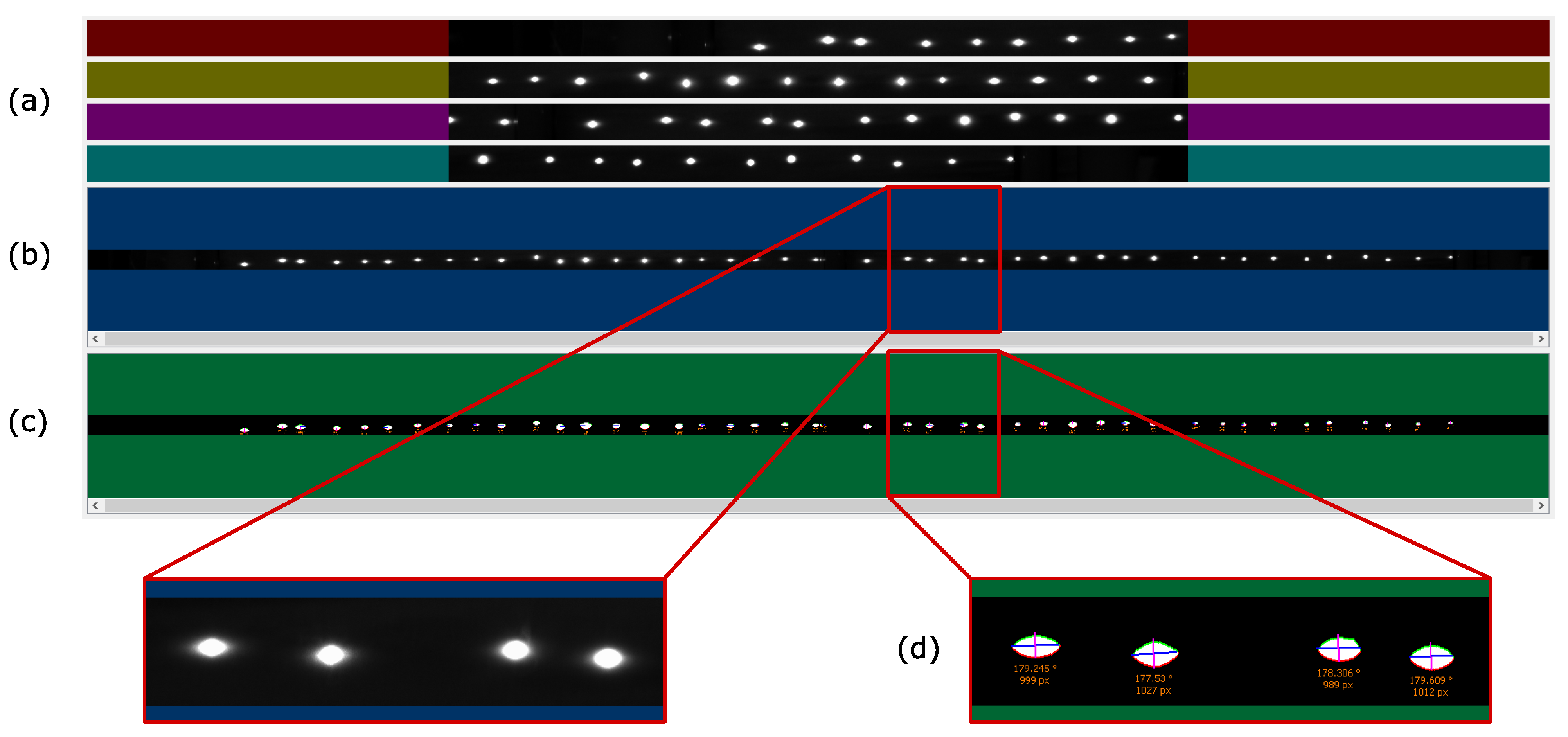
Fifty laser-dot modules with an output power of 5 mW each which project circular beams on veneers. They are positioned in line at a constant distance in the full 800 mm width of the peeling line, fixed on a support above it, and are thus perpendicular to the direction of the band and parallel to the main direction of the grain. Each laser-dot module is individually calibrated in order to provide a radiant flux of 0 to 5 mW (1 mW selected for Douglas fir) calibrated by a laser photodiode (Thorlab PM16-151). This power can be adapted according to the type of wood considered.

-

Four cameras (Basler acA2440-75 μm), performing video acquisition of the reflected ellipses on the veneer surface. Their resolution is of 2048 pixels in the width of the line (or the main direction of the grain) and 120 pixels in the scrolling direction of the band (perpendicular to the main direction of the grain). The maximal acquisition rate is 1000 frames/s.

The measurement resolution in the main direction of the fibers (perpendicular to the conveyor) was about 16 mm, corresponding to the mean distance between each laser-dot module. The measurement resolution across the main fiber direction depends on the aquisition speed of the cameras and on peeling line veneer conveyor speed. For the linear cutting speed of 1.5 m.s⁻¹ applied here to Douglas-fir veneer peeling, it was close to 3.5 mm. The 16 mm by 3.5 mm spatial resolutions obtained along and across the grain direction, respectively, can be compared to those of sawmill scanners, for which the corresponding resolutions are typically 1 mm in the length of the boards and 4 mm crosswise. A large difference in the resolution along main fiber direction according to the conveying direction was notable. In the main fiber direction, it was necessary to use a distance of 16 mm between the lasers so that the centers of the ellipses were not too close to avoid superimposing parts of ellipses. In the conveying direction, due to the movement of the veneers imposed by the linear speed of the line, ellipse shape information was obtained at different times, allowing for a much finer resolution (see Figure 2). Thus, in this direction, it was the acquisition frequency of the camera that drove the spacing of the ellipses.

Moreover, it should be noted that 3 belts ensured the conveying of the veneers along the line in the field of lasers and cameras (see Figure 1b,c). This therefore deprived the measurements of operating areas globally in the center and at the ends of the veneers. These laser points were therefore removed from the raw data.

A series of processing steps were required to convert the video raw data into a regular fiber orientation grid. The video information streams containing the raw data from the 4 cameras (Figure 2a) were recomposed into 1 as shown in Figure 2b. The processing of the superposition zones of the field of view of the cameras between them was carried out to guarantee the accuracy of the information over the entire width of the peeling line. A binarization of the images was then applied to detect the ellipse shapes (Figure 2c). In this study, the binarization threshold was adjusted for each peeled log as low as possible in order to obtain the largest possible ellipse areas without superimposition of the ellipses.

Veneer detection was performed by analyzing each of the images of the recorded ribbon: the increases without discontinuity in the average gray tone of the images corresponding to the passage of a light veneer over the dark background. Thus, each veneer was flagged by a beginning and an end in the temporal flow of the video, corresponding to a position and length in the ribbon once the veneer conveyor speed was taken into account. Processing was realized with the “FitEllipse” function of the OpenCV library [20] to enable the detection of ellipses and their orientations. This function calculates and provides the vertical and horizontal position of the center of the ellipse and the length of the large and small axis of the ellipse, as well as its angle with respect to the main direction of the fibers (Figure 2d). At the end of this first step of digital processing, 2 types of files were generated: a grayscale image for each veneer and a file containing information on the positioning and parameters of the ellipses.

After being cut by the clipper, veneers can slightly rotate during the conveyance. Thus, there was a second step of processing aiming at correcting the information by moving from the cameras coordinate system from the LOOBAR to the local coordinate system of the veneer. The detection of the cut edges and a conversion from px to mm allowed an angular correction of the fiber orientation values and a rotation of the grayscale image in order to visualize the veneer in its own local coordinate system (Figure 3a), with x_green being the position of a pixel in the longitudinal main direction of the veneer, and y_green being the position of a pixel in the tangential main direction of the veneer. This step allowe for the exploitation of the information even if the veneer coordinate system is not aligned with the coordinate system of the measurement apparatus.

Finally, the outputs of the LOOBAR scanning after these processing steps were as follows:

• x_green, the position of ellipses center along the grain direction in the veneer coordinate system (mm);
• y_green, the position of ellipse centers along the perpendicular axis to the grain direction in the veneer coordinate system (mm);
• θ, the angle (°);
• major and minor diameters (mm) that enable ratio calculation (dimensionless quantity); and
• the ellipse area (mm²).

These first 3 bullet points are shown in Figure 3b.

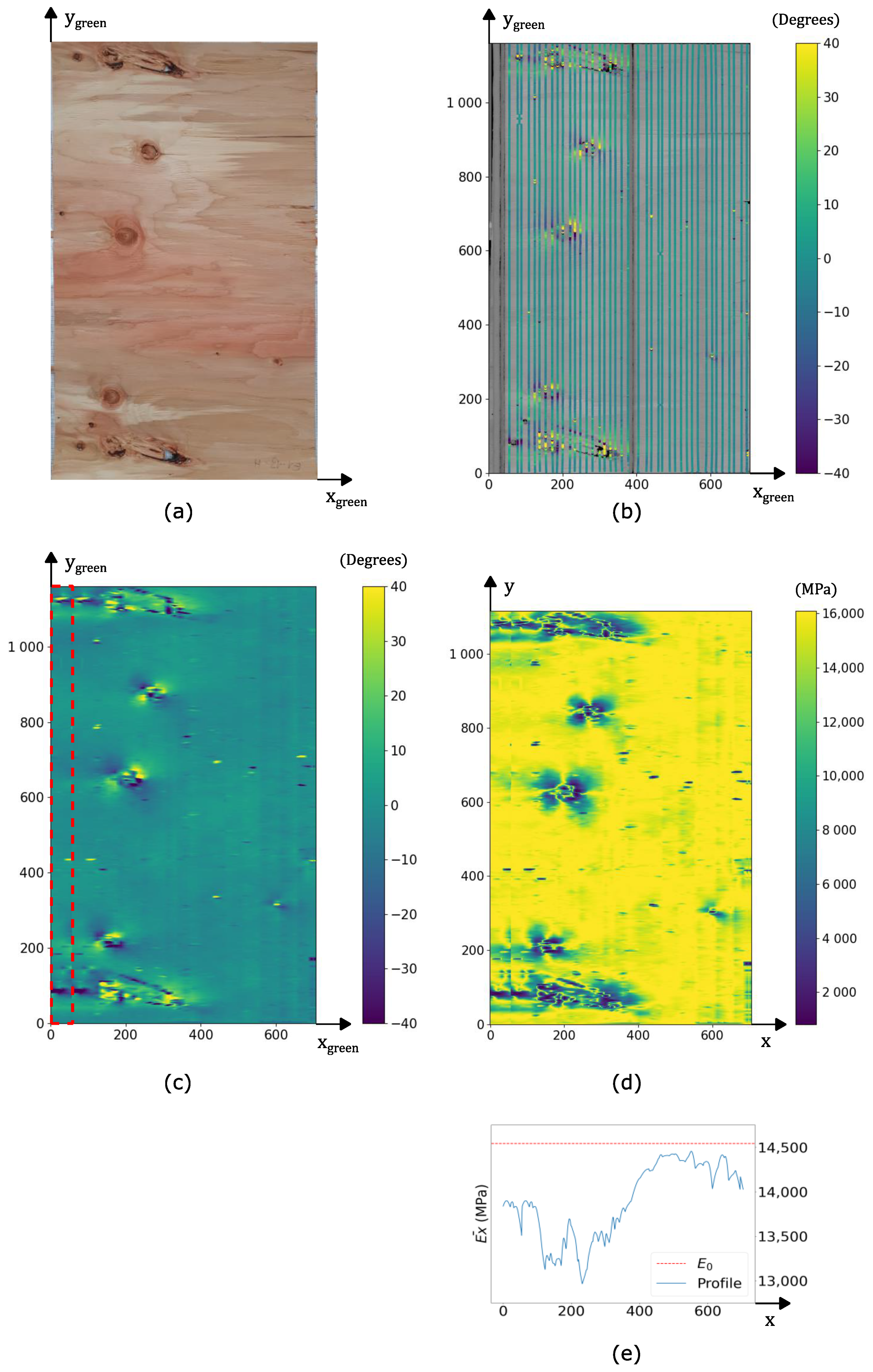
2.3. From Local Fiber Orientation to Stiffness Regular Grid

From LOOBAR outputs it was possible to obtain a standard-property grid at 12% moisture content to conform to structural standard.

A local fiber orientation regular grid was extracted for each veneer, and then a linear interpolation of the measured raw data points corresponding to the centers of the ellipses over their entire surface (Figure 3c) was undertaken to obtain a regular grid with an X by Y resolution, as in [15]. The fiber deviation area was clearly visible in the vicinity of knots, with a positive or negative deviation that was almost symmetrical around them, as widely described in [15]. For the veneer ends with no angle data due to the presence of belts, a compensation algorithm was therefore developed for the problem of empty areas of mechanical properties in the manufacturing of numerical panels and beams (see Section 2.6). The adopted method consisted of replicating the contiguous zones in the empty zones and duplicating them (visible in red box of Figure 3c). Concerning the missing data due to the belts, as far as the central belt area was concerned, the applied interpolation enabled us to overcome the problem.

Using the regular grid of fiber orientation measurement of each veneer, the calculation of a local elastic modulus was performed in 2 steps following the method developed in Viguier´s study [14]. First, the average density of the veneer was calculated. The mass of each veneer was weighed after drying at 9% with an accuracy of 0.1 g. For the calculation of the volume of the veneers, the nominal peeling thickness was used. The length and width at the green state were determined individually by manually cropping the grayscale images to the dimensions of each veneer ($\pm$5 mm). For width, the average shrinkage coefficient from the Tropix database [21] was applied according to the tangential orthotropic direction of the wood to adjust the volume to 9% moisture content. As a result, the veneer density was computed using Equation (1), including a 12% moisture content correction from the standard EN 384 [22].

$$\overline{{\rho }_{veneer}}=\frac{m_{veneer,9\%}}{L_{veneer,green} l_{veneer,9\%} e_{veneer,green}}\times \left[1-0.005\left(9\%-12\%\right)\right]$$

(1)

where

• ρ_veneer is the veneer average density (kg·m⁻³) at 12% moisture content;
• m_veneer,9% is the veneer global mass at 9% moisture content (kg);
• L_veneer,green and e_veneer,green are respectively the length and the thickness of the veneer at the green state (mm); and
• l_veneer,9% is the veneer width at 9% moisture content (mm).

The influence of density on E₀, the theoretical elastic of modulus for a straight grain, was computed according to Pollet [23], who studied clear Douglas-fir wood specimens by differentiating between juvenile and mature wood. Only the mature wood equation was used in this study because: (1) sapwood does not contain juvenile wood, and (2) the peeling operation leaves a core of wood at the pith with a diameter of 70 mm, which certainly contains almost exclusively juvenile wood concerning heartwood. Taking into account that the juvenile limit is usually observable for a cambial age of 15 years and by considering a mean radial growth of 5 mm for Douglas fir, a 75 mm diameter area from pith was obtained. Beyond this was the transition zone and mature wood. Equation (2), with 12% moisture content, is as follows:

$$E_0=36.605\overline{{\rho }_{veneer}}-4242.4$$

(2)

where

• E₀ is the theoretical elastic of modulus for straight grain (MPa); and
• ρ_veneer is the veneer average density (kg·m⁻³) at 12% moisture content.

The effect of the local fiber orientation, noted as θ(x,y), on the local modulus of elasticity in the longitudinal main direction of the veneer, denominated as E_x(x,y), was taken into account using Hankinson’s formula (Equation (3)) [24], with parameters according to Wood HandBook data [25]:

$$E_x\left(x,y\right)=E_0\frac{k}{{\sin }^n\left(\theta \left(x,y\right)\right)+k\times {\cos }^n\left(\theta \left(x,y\right)\right)}$$

(3)

where

• θ(x,y) is the local fiber orientation angle (°) in the veneer coordinate system;
• k is the ratio between the perpendicular to the grain (E₀) and the parallel to the grain modulus of elasticity (E₉₀); it was taken as equal to 0.05, in accordance with [25], specifically for Douglas fir; and
• n is an empirical determined constant. It was taken as equal to 2, as recommended in [25] concerning the modulus of elasticity.

In order to be consistent with the actual 12% moisture content veneer density, the regular grid had to be resized to 12% moisture content dimensions. Thus, the average tangential shrinkage coefficient from the Tropix database [21] was applied for according to the orthotropic direction of the wood to adjust the veneer regular grid width. A regular grid of local modulus of elasticity at 12% moisture content for each veneer was finally obtained (Figure 3d). This consideration of shrinkage for veneer regular grid dimensions explains the change in the coordinate system from (x_green, y_green) to (x,y) and the reduction in height of Figure 3d according Figure 3c.

From $E_x\left(x,y\right)$ the averaged local modulus of elasticity on all veneer surface was calculated to provide a criterion to estimate the global quality of the veneer according Equation (4).

$$\overline{E_{veneer }}=\frac{{{\displaystyle \sum }}_{x=1}^{n_x}{{\displaystyle \sum }}_{y=1}^{n_y}{E}_x\left(x,y\right)}{n_x{n}_y}$$

(4)

where

• n_x is the number of pixels in the $\stackrel{\rightharpoonup }{x}$ direction; and
• n_y is the number of pixels in the $\stackrel{\rightharpoonup }{y}$ direction.

The normalized Hankinson mean value, which will be also evaluated in this study to provide a criterion on fiber orientation, is given as follows (Equation (5)):

$$\overline{H_{veneer}}=\frac{{{\displaystyle \sum }}_{x=1}^{n_x}{{\displaystyle \sum }}_{y=1}^{n_y}\frac{k}{{\sin }^n\left(\alpha \left(x,y\right)\right)+k\times {\cos }^n\left(\alpha \left(x,y\right)\right)}}{n_x{n}_y}$$

(5)

This criterion is equal to 1 when the fiber orientation is perfecty longitudinal and tends to $k$ when all fibers are perpendicular to the $\stackrel{\rightharpoonup }{x}$ direction in the veneer coordinate system.

2.4. From a Regular Grid to an Equivalent Longitudinal Stiffness Profile

Veneers are used in LVL beams where the veneer orientation is mostly all along the beam length. Thus, the longitunal modulus of elasticity is the main parameter for sorting the veneers. To sort them efficiently, an equivalent longitudinal stiffness profile was determined for each of the veneers.

The stiffness profile of each veneer, visible in Figure 3e, was obtained by averaging the modulus of elasticity values along the $\stackrel{\rightharpoonup }{y}$ direction, as calculated in Equation (6).

$$\overline{E_x}\left(x\right)=\frac{{{\displaystyle \sum }}_{y=1}^{n_y}{E}_x\left(x,y\right)}{n_y}$$

(6)

where n_y is is the number of pixels in the $\stackrel{\rightharpoonup }{y}$ direction.

Coarsely, the general elevation of the profile is given by the density, which affects the E₀ value (red dashed line in Figure 3e), and downward peaks are symptomatic of the presence of knots. These peaks are all the more important because knots are mostly aligned along the same x coordinate as they come from the same crown branch, as shown by the blue curve in the example of Figure 3e.

Tukey´s HSD tests were performed to compare the criteria relative to each other.

2.5. Veneer Sorting and Grading

Two different ways to grade veneers are compared here based on appearance criteria on one hand, and based on average density and local fiber orientation on the other hand. This section describes each sorting and grading process.

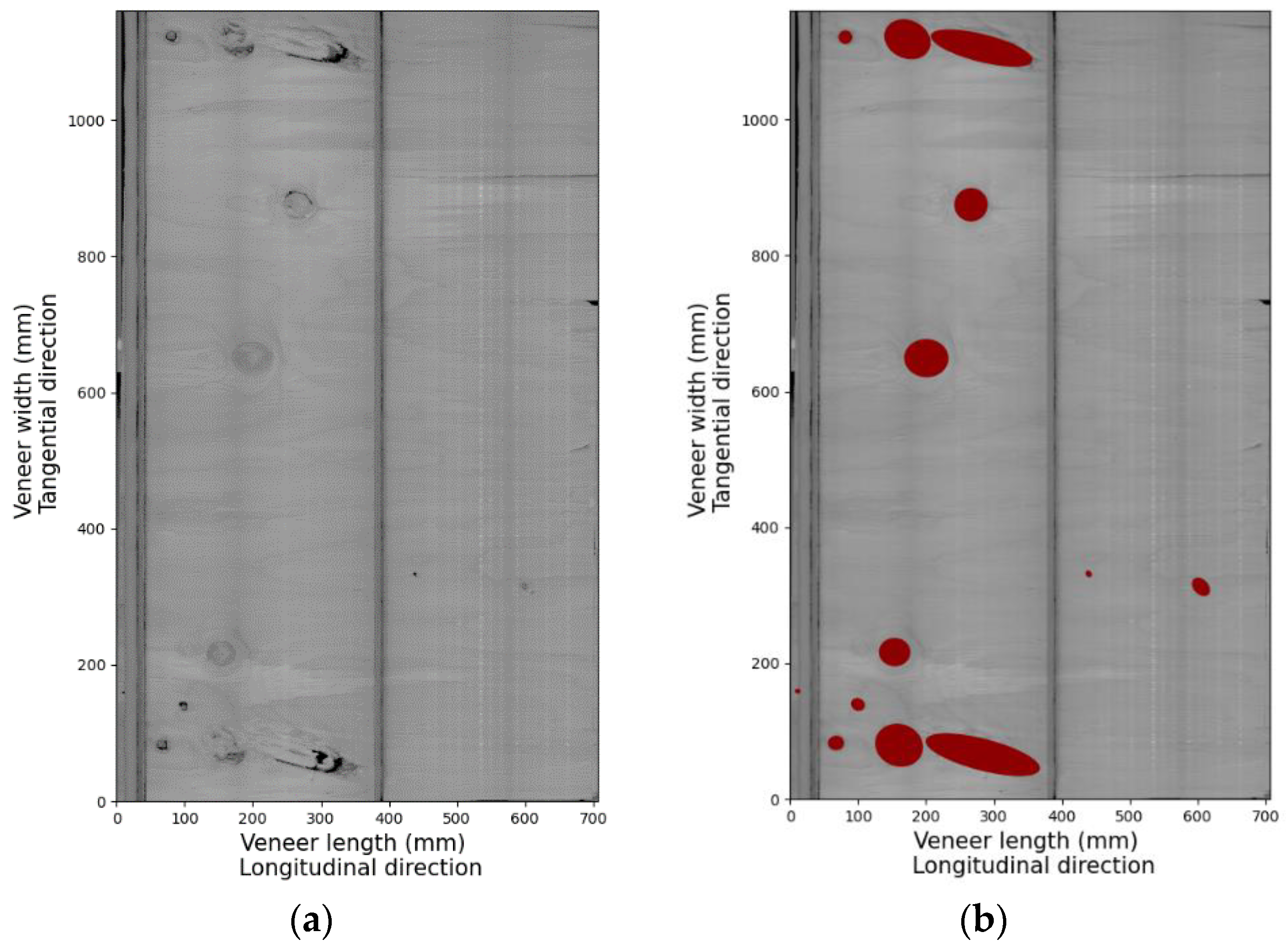
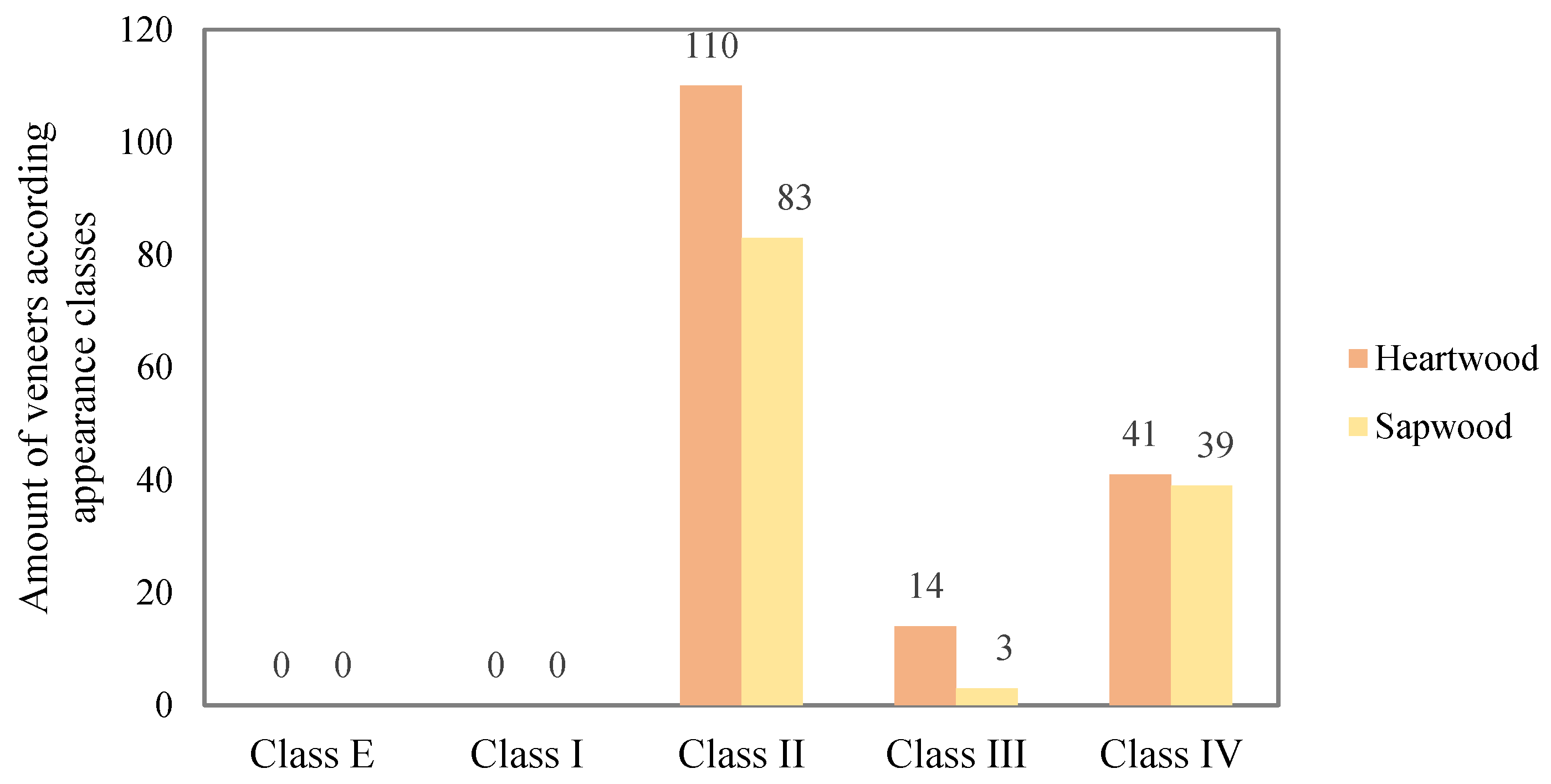
2.5.1. Appearance Grading

Cropped grayscale images (Figure 4a) from the LOOBAR cameras were used to detect the knots of the veneers. Each veneer was processed manually using open source ImageJ image processing and analysis software [26]. Knots were identified by the grayscale nuance difference with clear wood and were then approximated by ellipses (Figure 4b).

Information regarding the centroïd coordinates ($x_c$,$y_c$) and the major and minor diameter (${\varphi }_{ma},{\varphi }_{mi}$), as well as the angle of the major diameter, was saved and stored. This detection of knots for each veneer allowed for the calculation of 2 criteria:

-

n_k, the number of knots per veneer; and

-

KSR (knot surface ratio), defined as the ratio of cumulative knot areas to the total veneer area (Equation (7)),

$$KSR=\frac{{{\displaystyle \sum }}_{k=1}^{n_k}{A}_k}{A_v}$$

(7)

where

• A_k is the individual area of a knot (mm²); and
• A_v is the area of the veneer (mm²).

Veneers were sorted by considering the major diameter of the larger knot of each veneer. The classes of diameter were defined on the basis of EN 635-3 [2] criteria for adherent knots. After veneer drying, the knots were actually very brittle and close to be loose, but these criteria were better adapted to the population of diameters than the loose knots criteria of EN 635-3 which were designed for esthetic purposes. The classification conditions used are summarized in

Table 3. Appearance grading classes from the EN 635-3 standard.

Categories of Characteristics	Appearance Grading Classes
	E	I	II	III	IV
Very small knots	3/m2 permitted	Permitted
Sound and adherent knots	Almost absent	Permitted up to an individual diameter of:
		15 mm as long as their cumulative diameter does not exceed 30 mm/m2	50 mm	60 mm	Permitted

.

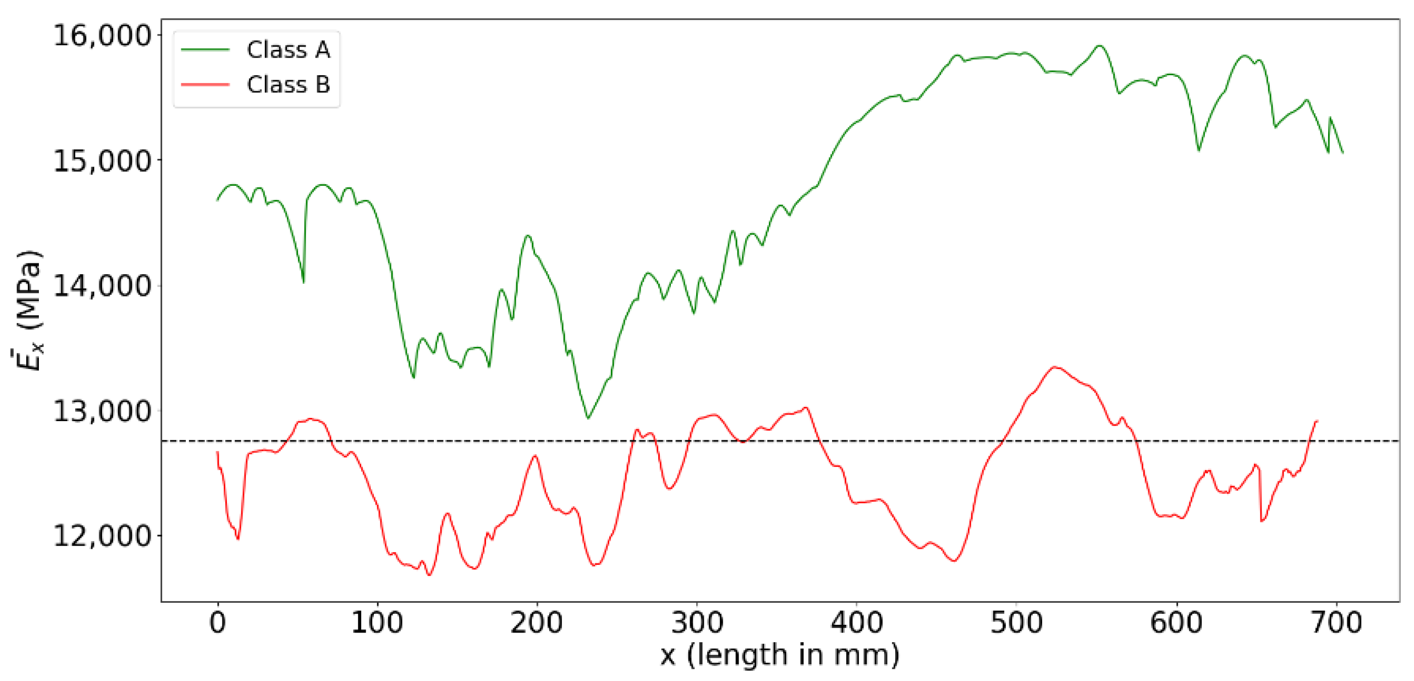
2.5.2. Modulus of Elasticity Profile Sorting

The aim was to no longer sort the veneers according to esthetic criteria but to use the composition of local fiber orientation and average density information. The stiffness profile of Equation (4) was used for sorting. In this study, a method was proposed that uses the minimum stiffness profile value of each veneer as the sorting criterion (Equation (8)).

$${\overline{E_x}}_{min}=\min \left(\overline{E_x}\left(x\right)\right)$$

(8)

The value of this indicator is not impacted by the principle of replicated strips on the sides of veneers to fill in the lack of measurement. From a profile point of view, portions of the profile are replicated, which does not change the value of the general minimum.

Veneer classes were thus established. Two classes were envisaged: the high-quality class A and low-quality class B. Class A included veneers for which the elastic modulus profile minimum was superior than a given threshold over its entire length (green curve in Figure 5). Class B included veneers in which the elastic modulus profile minimum was lower than the threshold (red curve in Figure 5).

A definition of a modulus of elasticity threshold between classes A and B is therefore necessary. Several thresholds can be defined according to the objectives of the manufacturer. Only 1 example has been retained for the present work. This threshold is the mean value of the minimum veneer stiffness profiles of the considered veneer population, defined by Equation (9). ${\overline{E_x}}_{min,v}$ is considered as the ${\overline{E_x}}_{min}$ value of a veneer v among a number of veneers $n_v$ of a sample.

$$E_T=\frac{{{\displaystyle \sum }}_{v=1}^{n_v}{\overline{E_x}}_{min,v}}{n_v}$$

(9)

where n_v is the number of veneers of the considered sample.

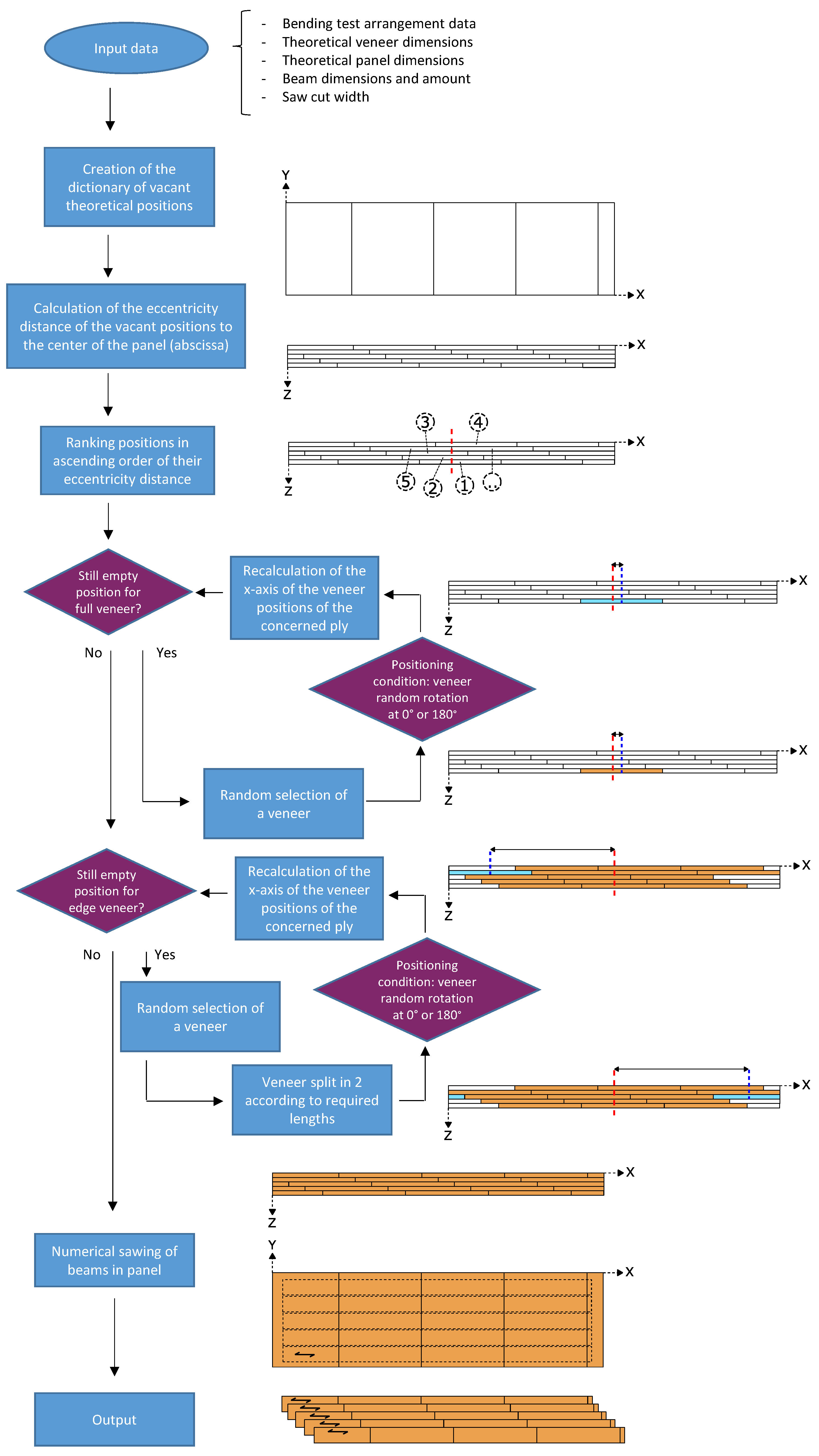
2.6. LVL Panel Composition by Random Veneer Placement

In order to assess the mechanical properties of typical LVL-P beams made of a given class of graded veneers, an algorithm was developed based on the random placement of 60 actually measured veneers in the multi-ply material to simulate the manufacturing of a 15 ply LVL-P type panel. Assuming the thickness of each veneer as exactly 3 mm, this leads to a panel thickness of about 45 mm, which is a typical thickness for LVL-P [1]. The modeled panel length was 3000 mm (obtained by using 4 veneers per ply), so there was a total of 60 veneers per panel.

The algorithm steps are summarized in Figure 6. First, the input data were filled in: theoretical veneer dimensions (clipper width, peeling thickness, distance between scratcher knives), number of plies in the panel, the number of beams to be cut into the panel and their nominal dimensions. A sequence of stacking, listing all theoretical vacant positions where veneers would be assigned, was then created. To compose this sequence, a single theoretical length of veneer in the main grain direction (L_theo) was used. This corresponds to the distance between the scratcher knives which define the length of the veneers when peeling the logs. From 1 ply to the next a 1/5 length offset in the sequence of the theoretical length from the abscissa origin was performed. This offset from 1 ply to another, as for industrial classical products, aimed to avoid superimposing the veneer jointing areas and ensure the cohesion of the material. A 1/5 ratio is a good compromise between a too-small offset and a too-premature redundancy of the butt joint area.

In this study, the panel was composed of 60 veneers composed of 72 positions considering veneers at the extremities that were cut in half. In the initial state, the following theoretical information was available for each of the vacant veneer positions (for i from 1 to 72):

-

$\overrightarrow{X}$: the axis parallel to the main orientation of the fibres in the panel;

-

X_i,min,theo: in the panel system of the axis, this is the minimum abscissa of the theoretical position of veneer position number I;

-

X_i,max,theo: in the panel system of the axis, this is the maximum abscissa of the theoretical position of veneer position number i. For each vacant full veneer position, there is $L_{theo}=X_{i,max,theo}-X_{i,min,theo}$;

-

The ply number (between 1 and 15 for these 15 ply panels); and

-

X_{i,eccentricity,theo}: The eccentricity distance. This is the distance between the abscissa of the centre of the panel and the centre abscissa of the theoretical position of the veneer position number i (Equation (10)).

$$X_{i,eccentricity,theo}=\left|-X_{i, centerpanel, theo}+\left(X_{i,min,theo}+\frac{ X_{i,max,theo}-X_{i,min,theo}}{2}\right)\right|$$

(10)

Each of the positions in the panel was initially considered as available. All vacant positions were first classified in ascending order according to their eccentricity distance. The first vacant position to be assigned was that with the lowest absolute value of the eccentricity distance. This method allowed us to start the algorithm by using full-length veneers, whereas at the ends of the panels many veneers had to be cut (cf. Figure 6). At each loop iteration a veneer was randomly selected from the list and placed in a vacant position. A random choice between placing the veneer at 0° or 180° was made at this step. Each time a veneer was allocated to a position, the theoretical abscissa of the vacant positions was recalculated from its real length, L_veneer. The difference between the theoretical length of the vacant position L_theo and the actual proper length of the veneer L_veneer assigned to it creates a offset, requiring the offset of the following veneer vacant positions in the concerned ply for each loop. Once all the positions requiring full-length veneers were assigned, the end veneers were in turn completed. For simplicity, when a veneer attributed to a ply was cut in 2 parts as required, each of its 2 parts completed both ends of the ply. Again, for each part of veneer the condition of 0°/180° for positioning was applied. Once all veneers had been assigned and therefore all plies of the material panel were filled, numerical sawing of the beams in the panel was performed according to the parameterized dimensions.

In this study, for each set of 60 veneers, 150 random panels were simulated. In order to evaluate their bending stiffness, each of them was virtually cut into 5 LVL-P beams of 145 mm in width. This width was chosen to cut beams with the minimum of 18 times the beam height between the lower support ratio from manufactured panels.

2.7. Mechanical Properties of Randomly Composed LVL Panels and Beams

This section details the calculation of the criterion used to quantify the mechanical bending performance of the beams randomly generated in bending.

In a first step, the E_ply(x,y) value of each ply composing the beam was averaged along the $\stackrel{\rightharpoonup }{z}$ direction to obtain the grid $\overline{E_{beam}}\left(x,y\right)$of the modulus of elasticity along the $\stackrel{\rightharpoonup }{x}$ and $\stackrel{\rightharpoonup }{y}$ direction of each beam according to Equation (11):

$$\overline{E_{beam}}\left(x,y\right)=\frac{{{\displaystyle \sum }}_{n=1}^{n_{plies}}{E}_{ply,n}\left(x,y\right)}{n_{plies}}$$

(11)

where n_plies is the total number of plies in the $\stackrel{\rightharpoonup }{z}$ direction.

An effective bending stiffness, EI_eff, was calculated for each section of 1 pixel of height in the $\stackrel{\rightharpoonup }{y}$ direction along the $\stackrel{\rightharpoonup }{x}$ direction of the LVL beams in accordance with Equation (12):

$$E{I}_{eff}\left(x\right)={\displaystyle \sum }_{y=1}^{n_y}\left(\overline{E_{beam}}\left(x,y\right)I_{gz,\Delta y}+\overline{E_{beam}}\left(x,y\right)A_{\Delta y}{d}_{\Delta y}{\left(x\right)}^2\right)$$

(12)

with

$$\begin{gathered} I_{gz,\Delta y}=\frac{L_{beam}\times {\left({\Delta }_y\right)}^2}{12} \\ {A}_{\Delta y}=L_{beam}\times {\Delta }_y \end{gathered}$$

where

• n_y is the number of pixels in the $\stackrel{\rightharpoonup }{y}$ direction;
• I_gz,Δy is the second moment of area of the section of Δ_y height at a given x position;
• A_Δy is the area of the section of Δ_y height at a given x position; and
• d_Δy is the distance from the neutral fiber of each element. This was calculated at a given x position and took into account the modulus of elasticity variation in the section, as explained in [14].

An equivalent modulus of elasticity, $E_{eq}$, was calculated according Equation (13), to establish a bending criterion for ranking the beams over their entire length.

$$E_{eq}=\frac{n_x}{ I_{gz}{{\displaystyle \sum }}_{x=1}^{n_x}\frac{1}{E{I}_{eff}\left(x\right)}}$$

(13)

$E_{eq}$ was chosen as the performance indicator for the bending beam because it considers the entire length of the beam in its calculation without considering a specific bending solicitation. Its calculation considers each elemental effective bending stifness at an x given position as being in a series along the entire length of the beam. The calculation of the equivalent module follows the same principle as that of an equivalent rigidity of several springs in a series. $\overline{E_{eq}}$ is considered as the $E_{eq}$ mean value of beams in a given sample.

3. Results

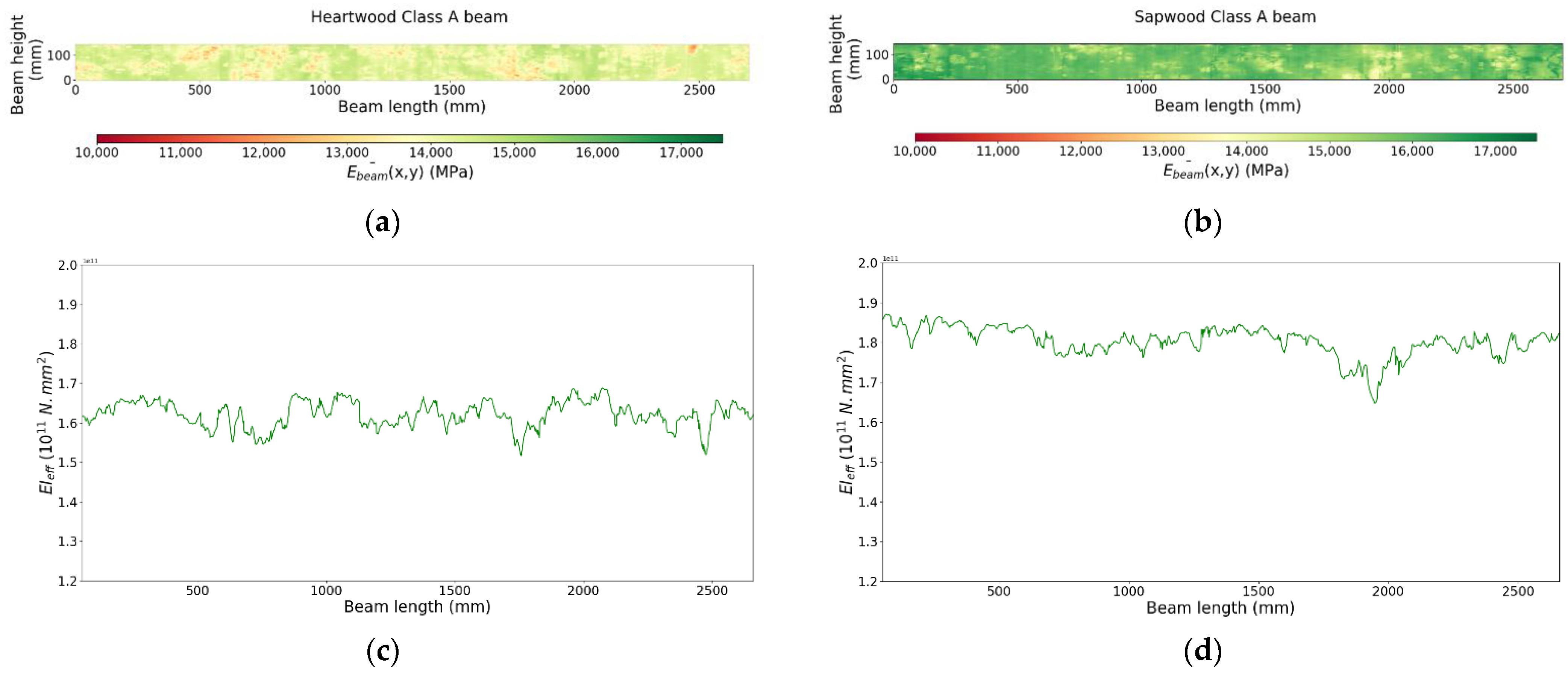
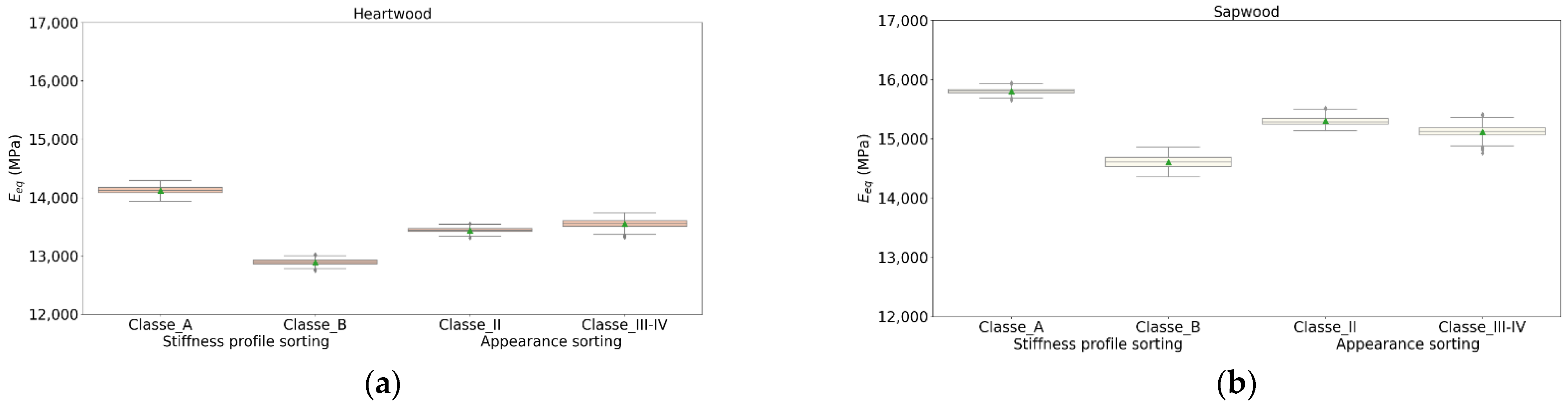
3.1. A Comparison of Two Sorting Methods

3.1.1. Appearance Sorting

In total, 286 studied veneers were sorted according to the criteria considered in Section 2.5.1 from the EN 635-3 standard [2] relative to knottiness. A differentiation between heartwood and sapwood was also made to highlight distinctions regarding the impact of their morphological and physico-mechanical properties on the modeled performance of LVL products. Figure 7 shows the results of the number of veneers in each appearance class.

In the veneer sample there were no veneers in Classes E and I, as the criteria for knot size and concentration are very restrictive. This is very typical of veneers from large Douglas-fir trees for which large knots are very common. Class III is very low fill (14 veneers for heartwood, 3 for sapwood, or 5.9% of total amount of veneers). This was due to the standard that permits individual diameters of knots up to 60 mm, while in Class II they are permitted up to 50 mm. In other words, the largest knot of the veneer must be between 50 mm and 60 mm. This criterion was very restrictive as compared to that of Class IV, which allowed diameters of 60 mm and above. With regard to the proportion of heartwood and sapwood in Classes II and IV, it was not possible to draw conclusions regarding the relationship between the distance to the pith of each type of wood and knot sizes because the numbers of total veneers of sapwood and heartwood were different. Given the small number of veneers contained in Class III, the data from these veneers were regrouped with Class IV for the sake of simplicity.

Tukey´s HSD test was performed to compare both the appearance criteria and computed criteria with the LOOBAR (

Table 4. Data from appearance classes.

		Heartwood Mean Value (CoV%)		Sapwood Mean Value (CoV%)
	Units	Class II	Class III/IV	Class II	Class III/IV
Amount of knots	/	20 (47) a	16 (39) b	9 (40) c	7 (32) c
KSR	%	0.58 (59) b	1.79 (25) a	0.28 (47) c	1.71 (45) a
$\overline{{\rho }_{veneer}}$	kg/m3	503 (4.8) d	531 (5.2) c	553 (4.5) b	571 (5.4) a
$\overline{H_{veneer}}$	d.q.	0.936 (3.7) b	0.887 (3.9) c	0.950 (3.5) a	0.896 (4.8) c
$\overline{E_{veneer}}$	MPa	13,276 (7.1) b	13,492 (7.9) b	15,207 (6.7) a	14,930 (8.8) a

Values followed by a different letter within a column are statistically different at p-value = 5% (ANOVA and Tukey´s HSD test).

). Populations submitted to an HSD test (Tukey´s method) are signaled in the following tables by a lowercase letter. In order to facilitate the reading, a color code for each line was added to highlight the significantly different values (p-value < 0.05) line by line: green for the highest value, red for the lowest value.

First of all, we can make observations based on knottiness. The KSR value was higher in the lower-quality Class III/IV than in Class II for both heartwood and sapwood, is consistent with the principle of appearance grading. It appears that there were fewer knots in Class III/IV than in Class II for heartwood. For sapwood, the HSD test showed that there were no significant difference in the number of knots between Class II and Class III/IV veneers. There were fewer knots in sapwood than in heartwood, whereas the KSR values in Class III/IV were similar, showing that sapwood knots were much bigger that heatwood knots, which is consistent with the increasing diameter of a branch along with the growth of the tree.

Sapwood density was higher than that of heartwood, which is a classical effect due to density increase with the distance to the pith within the tree. More surprisingly, for both heartwood or sapwood the average veneer density of Class III/IV was significantly higher than that of Class II. This result may be explained by two effects:

• The appearance sorting method select veneers with larger knots for the lower-quality Class III/IV. Veneers located far from the pith of the tree should arise (otherwise branches are not large enough). This is wood with a higher density, for the same reason as explained before.
• Knots are denser than in clear wood and higher KSR values can be observed for class III/IV.

For both sapwood and heartwood, the average standardized Hankinson criterion $\overline{H_{veneer}}$ values were higher for the higher-quality Class II. This criterion is calculated from the measure of local fiber orientation, the variation of which is mainly due to the presence of knots.

The sapwood $\overline{E_{veneer }}$was significantly higher than that of heartwood, but when looking at the classes from each type of wood (+12.6% between $\overline{E_{veneer}}$ of each type of wood), there was no significant difference according to the HSD test. This can be explained by a compensation phenomenon between the fiber orientation information and density, which results in a lack of real variation of this parameter based on appearance sorting classes.

It can therefore be concluded that, in terms of $\overline{E_{veneer }}$for these studied batches, each appearance sorting class has similarly variable veneers. Sorting based solely on appearance may therefore not be the most efficient method because it does not take into account important parameters such as density, and it does not differentiate veneers with a few large knots from veneers with many smaller knots. Other sorting methods should therefore be considered.

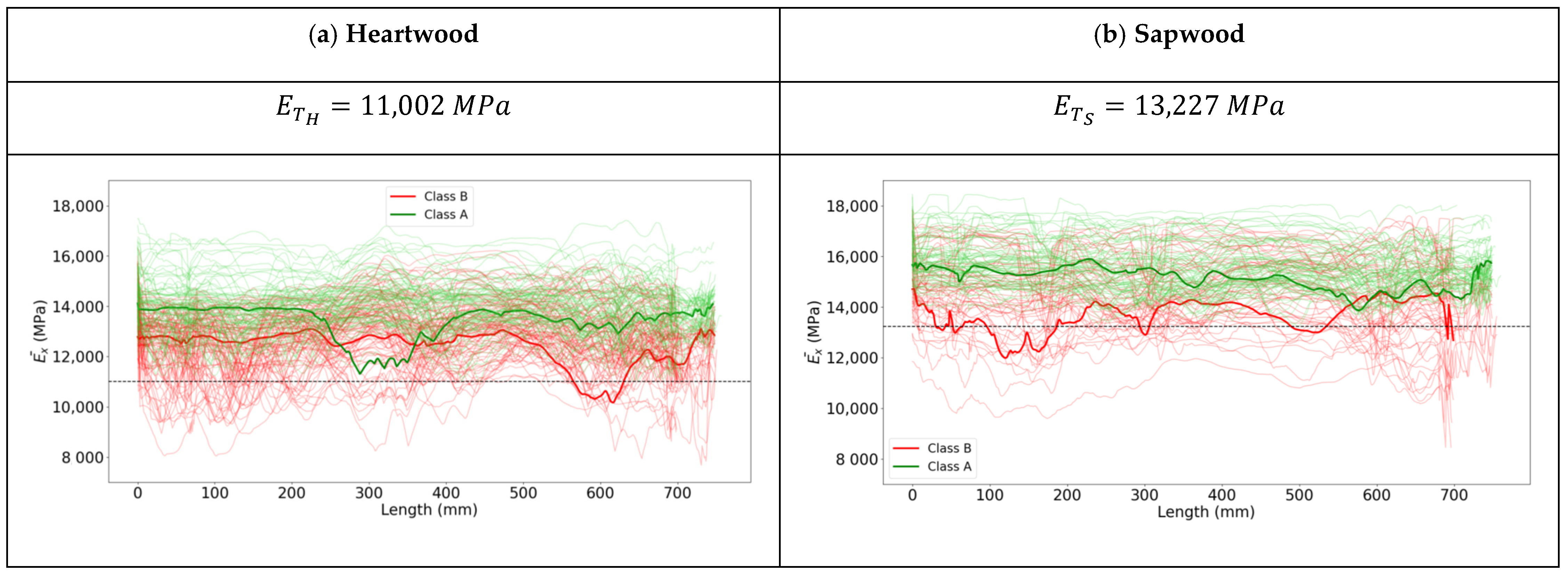
3.1.2. Stiffness Profile Sorting

The stiffness profiles of all the veneers colored depending on their class were calculated for sapwood and heartwood according to the minimum method, as shown in Figure 8. For the sake of clarity, only one profile of each class is shown in bold and dark colour, while the remaining veneers are shown with a finer width and a clearer color.

When performing appearance sorting, a single limiting knot is used to classify the veneer. By analogy, sorting by the limiting minimum value of the profile retains the same strategy. It is logical to note that the threshold was higher for sapwood than heartwood, since it was calculated from populations. Figure 9 shows veneer populations in Class A and Class B, including the proportion of each appearance sorting class. Since the threshold was the average of the individual minimum values of the veneer stiffness profiles, there was a logical balanced distribution of veneers between Classes A and B.

For heartwood, 76 veneers were distributed in Class A and 89 in Class B. For sapwood, 71 were in Class A and 54 in Class B. Similar proportions of appearance in Class II veneers were found in Classes A and B for heartwood (76.3%) and sapwood (80.3%). This implies, therefore, that 23.7% and 19.7% of appearance-sorted low-quality Class III/IV heartwood and sapwood veneers were incorporated into this new high-quality Class A. Conversely, 58.4% heartwood and 48.1% sapwood in appearance-sorted Class II veneers represented Class B. These results mean either that the distribution of the knots of these Class B veneers was concentrated in verticils, resulting in a minimum localized value, or that their density was in the low band. According to this approach (computed $\overline{E_x}\left(x\right))$ and chosen threshold, the appearance quality sorting is a very poor criterion for the grading of veneers from this Douglas-fir resource from a mechanical application perspective.

Table 5. Data from stiffness profile classes.

		Heartwood Mean Value (CoV%)		Sapwood Mean Value (CoV%)
	Units	Class A	Class B	Class A	Class B
Amount of knots	/	16 (43) b	21 (45) a	8 (36) c	8 (41) c
KSR	%	0.70 (82) b	1.22 (56) a	0.45 (98) c	1.16 (85) a
$\overline{{\rho }_{veneer}}$	kg/m3	523 (5.3) c	504 (5.2) d	563 (4.4) a	553 (5.7) b
$\overline{H_{veneer}}$	d.q.	0.941 (3.1) a	0.902 (4.7) b	0.953 (2.5) a	0.905 (5.7) b
$\overline{E_{veneer}}$	MPa	13,996 (5.8) c	12,784 (6.0) d	15,575 (5.0) a	14,479 (8.3) b

Values followed by a different letter within a column are statistically different at p-value = 5% (ANOVA and Tukey HSD test).

shows data regarding stiffness profile classes. This should be compared with Table 4.

It can be noted that the trends were no longer the same as those observed with appearance sorting. The upper class by stiffness profile (Class A) was now denser than the lower class (Class B) (+3.8% for heartwood, +1.8% for sapwood), whereas the reverse was true for appearance sorting classes (−5.3% and −3.1%, respectively). For the normalized Hankinson mean value $\overline{H_{veneer}}$criterion, Class A was always higher than Class B (+4.3% and +5.3%), but the differences were now logically less important than for appearance sorting (+5.5% and +6.0%). This trend was also logically followed for KSR. For the averaged local modulus of elasticity mean value $\overline{E_{veneer}}$, there were now significant differences between Class A and Class B. Class A had veneers with higher average values of +9.5% and +7.6%, respectively, with regard to Class B veneers. When sapwood veneers presented a higher $\overline{E_{veneer}}$ than heartwood, the Class A heartwood $\overline{E_{veneer}}$ value was 13,996 MPa, slightly higher than the Class II appearance value of 13,276 MPa.

3.2. Comparison of LVL Mechanical Performance According to Sorting Method and Classes

Figure 10a,b presents an example of a regular grid of the local modulus of elasticity averaged over the 15 plies ($\overline{E_{beam}}\left(x,y\right)$) of the LVL beam randomly generated from veneers classified in Class A that are relatively well homogenized.

Figure 10c,d shows an example of an effective stiffness profile of beams. Because of its overall constant appearance, this makes it possible to observe the homogeneity in terms of the EI_eff profile of the random placement of heterogenous veneers in the material.

In total, 150 random panels from each class were modeled, in which 5 beams were digitally cut. When a class had fewer than 60 veneers, some were doubled representatively of the forest plots and logs which composed the batches. These beams were then tested by the analytical calculation model. The aim was therefore to be able to compare the performance of beams composed of veneers from classes. $\overline{E_{eq}}$ was calculated for each class. Figure 11 shows results for each class.

In the case of profile sorting, the $E_{eq}$ results of panel beams made up of Class A veneers were higher than those of Class B beams. The consideration of fiber orientation and density in the grading methodology appears to be more effective because it reveals a better discrimination of qualities between upper and lower classes than the actual standard of appearance sorting.

To ensure the reliability of the $\overline{E_{eq}}$ results, 150 control random panels were generated for each class. It appears that for the results presented, the maximum relative difference between sample presented and control samples $\overline{E_{eq}}$ was always less than 0.2%.

For sapwood, it is noted that the beams from the Class A random panels, which is the top-graded class, had an $\overline{E_{eq}}$ that was 8.2% higher than that of the Class B random beams (15,805 MPa vs. 14,610 MPa). The difference between appearance-sorted Classes II and III/IV averaged 1.2% (15,301 MPa vs. 15,119 MPa). For heartwood, there was a 9.6% difference (14,126 MPa vs. 12,894 MPa) between Class A and Class B beams. By comparison, the difference between appearance-sorted classes II and III/IV was on average equivalent (13,442 MPa vs. 13,555 MPa). It can therefore be concluded that the sorting by stiffness profile is much more selective and nicely dissociates the product qualities from the local modulus.

It is interesting to put these results into perspective with those of Table 4 and Table 5. There was a very minor gap between the $\overline{E_{veneer}}$ of the veneers and the E_eq of the beams randomly modeled for each class, whether they were from visual sorting or profile sorting (maximum 1.4% relative gap).

4. Discussion

This article provides the first results of veneer sorting based on both fiber orientation and density considerations.

It was shown that veneer sorting by stiffness profile computed from fiber orientation measurement and density mean values theoretically leads to more efficient grading than appearance grading based on knottiness to obtain a higher stiffness. It is important to remember that this conclusion is based on modeling results that allowed us to obtain a large number of results, which would not be attainable by experimental tests (a total of 600 panels or 3000 beams were generated). However, the conclusion should be trusted because the mechanical model principles relies on a method which has been successfully applied to sawn timber [10,27]. Furthermore, in the second part of this series of articles [28], the present modeling method is successfully compared to experimental measurement with some very different testing configurations.

It should be noted that only one particular method to separate the batch of veneers in two classes has been tried, but many others could have been considered. In addition, the limited studied veneer population, especially by practicing a heartwood/sapwood differentiation, does not allow for the creation of more than two classes. With more veneers and even more varied forest stands, more classes would be possible. This could take place for instance by using a percentile of stiffness instead of the mean value or global value, which can rely on strength classes (EN 338 standard [29]). In this article, the “minimum method”, based on the analogy of appearance grading, may not be sufficient. Use of the stiffness profile minimum and the MOE mean value of veeners computed into a single multi-criteria score may be better.

This sorting method, based on the modeling of local mechanical properties by density and local fiber orientation measurement, offers very interesting potential for the peeling industry. Since the thresholds are calculated from measured veneers, a two-step procedure for implementing this sorting method could be proposed. An initial phase of representative resource measurement for considered species could be performed to calculate the thresholds. Sorting could then be implemented, and the calculation of thresholds refined by the continuously generated data. The moisture-sorting process existing in the industry, which allows for the discrimination of heartwood and sapwood, can be seen has a form of quality sorting in itself, which can lead to dissociated application fields. Heartwood, due to its durability, can be used in outdoor structures such as bridges. Sapwood, with better intrinsic properties due in part to its higher density, it can be used in heavy-stressed indoor or outdoor construction with the application of protective products.

References

1. LVL Handbook Europe; Federation of the Finnish Woodworking Industries: Helsinki, Finland, 2019.
2. NF EN 635-3. Plywood. Classification by Surface Appearance. Part 3: Softwood. 1 July 1995. Available online: https://sagaweb-afnor-org.rp1.ensam.eu/fr-FR/sw/consultation/notice/1244973?recordfromsearch=True (accessed on 29 October 2020).
3. Faydi, Y.; Viguier, J.; Pot, G.; Daval, V.; Collet, R.; Bleron, L.; Brancheriau, L. Modélisation des propriétés mécaniques du bois à partir de la mesure de la pente de fil. In Proceedings of the 22e Congrès Français de Mécanique, Lyon, France, 24–28 August 2015. [Google Scholar]
4. Viguier, J.; Marcon, B.; Girardon, S.; Denaud, L. Effect of Forestry Management and Veneer Defects Identified by X-ray Analysis on Mechanical Properties of Laminated Veneer Lumber Beams Made of Beech. BioResources 2017, 12, 6122–6133. [Google Scholar] [CrossRef] [Green Version]
5. Nyström, J. Automatic measurement of fiber orientation in softwoods by using the tracheid effect. Comput. Electron. Agric. 2003, 41, 91–99. [Google Scholar] [CrossRef]
6. Simonaho, S.-P.; Tolonen, Y.; Rouvinen, J.; Silvennoinen, R. Laser light scattering from wood samples soaked in water or in benzyl benzoate. Opt.-Int. J. Light Electron Opt. 2003, 114, 445–448. [Google Scholar] [CrossRef]
7. Purba, C.Y.C.; Viguier, J.; Denaud, L.; Marcon, B. Contactless moisture content measurement on green veneer based on laser light scattering patterns. Wood Sci. Technol. 2020, 54, 891–906. [Google Scholar] [CrossRef]
8. Jehl, A.; Bleron, L.; Meriaudeau, F.; Collet, R. Contribution of slope of grain information in lumber strength grading. In Proceedings of the 17th International Nondestructive Testing and Evaluation of Wood Symposium, Sopron, Hungary, 14–16 September 2011. [Google Scholar]
9. Jehl, A. Modélisation du Comportement Mécanique Des Bois de Structures Par Densitométrie X ET Imagerie Laser. Ph.D. Thesis, ENSAM, Cluny, France, 2012. [Google Scholar]
10. Viguier, J.; Bourreau, D.; Bocquet, J.-F.; Pot, G.; Bléron, L.; Lanvin, J.-D. Modelling mechanical properties of spruce and Douglas fir timber by means of X-ray and grain angle measurements for strength grading purpose. Eur. J. Wood Wood Prod. 2017, 75, 527–541. [Google Scholar] [CrossRef] [Green Version]
11. Olsson, A.; Oscarsson, J.; Serrano, E.; Källsner, B.; Johansson, M.; Enquist, B. Prediction of timber bending strength and in-member cross-sectional stiffness variation on the basis of local wood fibre orientation. Eur. J. Wood Wood Prod. 2013, 71, 319–333. [Google Scholar] [CrossRef] [Green Version]
12. Hu, M.; Olsson, A.; Johansson, M.; Oscarsson, J. Modelling local bending stiffness based on fibre orientation in sawn timber. Eur. J. Wood Prod. 2018, 76, 1605–1621. [Google Scholar] [CrossRef] [Green Version]
13. Hu, M.; Johansson, M.; Olsson, A.; Oscarsson, J.; Enquist, B. Local variation of modulus of elasticity in timber determined on the basis of non-contact deformation measurement and scanned fibre orientation. Eur. J. Wood Wood Prod. 2015, 73, 17–27. [Google Scholar] [CrossRef]
14. Viguier, J.; Bourgeay, C.; Rohumaa, A.; Pot, G.; Denaud, L. An innovative method based on grain angle measurement to sort veneer and predict mechanical properties of beech laminated veneer lumber. Constr. Build. Mater. 2018, 181, 146–155. [Google Scholar] [CrossRef]
15. Frayssinhes, R.; Girardon, S.; Denaud, L.; Collet, R. Modeling the Influence of Knots on Douglas-Fir Veneer Fiber Orientation. Fibers 2020, 8, 54. [Google Scholar] [CrossRef]
16. Lutz, J.F. Heating veneer bolts to improve quality of Douglas-fir plywood. Report No. 2182. In Proceedings of the Section Meeting of the Forest Products Research Society, Bellingham, WA, USA, 8–9 February 1960. [Google Scholar]
17. Stefanowski, S.; Frayssinhes, R.; Grzegorz, P.; Denaud, L. Study on the in-process measurements of the surface roughness of Douglas fir green veneers with the use of laser profilometer. Eur. J. Wood Prod. 2020, 555–564. [Google Scholar] [CrossRef]
18. Mothe, F.; Marchal, R.; Tatischeff, W.T. Heart dryness of Douglas fir and ability to rotary cutting: Research of alternative boiling processes. 1. Moisture content distribution inside green wood and water impregnation with an autoclave. Ann. For. Sci. 2000, 57, 219–228. Available online: https://agris.fao.org/agris-search/search.do?recordID=FR2000003808 (accessed on 29 October 2020). [CrossRef] [Green Version]
19. NF-EN-322. Panneaux à Base de Bois-Determination de L’humidité. 1 June 1993. Available online: https://cobaz-afnor-org.rp1.ensam.eu/notice/norme/nf-en-322/FA020887?rechercheID=1757547&searchIndex=1&activeTab=all#id_lang_1_descripteur (accessed on 8 June 2021).
20. OpenCV. Available online: https://opencv.org/ (accessed on 11 June 2021).
21. Tropix 7. Les Principales Caractéristiques Technologiques de 245 Essences Forestières Tropicales-Douglas. 2012. Available online: https://tropix.cirad.fr/FichiersComplementaires/FR/Temperees/DOUGLAS.pdf (accessed on 29 October 2020).
22. NF EN 384+A1. Structural Timber-Determination of Characteristic Values of Mechanical Properties and Density. 21 November 2018. Available online: https://sagaweb-afnor-org.rp1.ensam.eu/fr-FR/sw/consultation/notice/1539784?recordfromsearch=True (accessed on 29 October 2020).
23. Pollet, C.; Henin, J.-M.; Hébert, J.; Jourez, B. Effect of growth rate on the physical and mechanical properties of Douglas-fir in western Europe. Can. J. For. Res. 2017, 47, 1056–1065. [Google Scholar] [CrossRef]
24. Hankinson, R.L. Investigation of crushing strength of spruce at varying angles of grain. Air Serv. Inf. Circ. 1921, 3, 16. [Google Scholar]
25. Forest Products Laboratory and United States Departement of Agriculture, Forest Service. Wood Handbook, Wood as an Engineering Material; General Technical Report FPL-GTR-190; Forest Products Laboratory and United States Departement of Agriculture: Madison, WI, USA, 2010. [Google Scholar]
26. ImageJ. ImageJ Wiki. Available online: https://imagej.github.io/software/imagej/index (accessed on 23 June 2021).
27. Olsson, A.; Pot, G.; Viguier, J.; Faydi, Y.; Oscarsson, J. Performance of strength grading methods based on fibre orientation and axial resonance frequency applied to Norway spruce (Picea abies L.), Douglas fir (Pseudotsuga menziesii (Mirb.) Franco) and European oak (Quercus petraea (Matt.) Liebl./Quercus robur L.). Ann. For. Sci. 2018, 75, 102. [Google Scholar] [CrossRef] [Green Version]
28. Duriot, R.; Pot, G.; Girardon, S.; Denaud, L. New perspectives for LVL manufacturing wood of heterogeneous quality—Part. 2: Modeling and manufacturing of bending-optimized beams. to be defined.
29. NF EN 338. Structural Timber-Strength Classes. 1 July 2016. Available online: https://sagaweb-afnor-org.rp1.ensam.eu/fr-FR/sw/consultation/notice/1413267?recordfromsearch=True (accessed on 29 October 2020).
Figure 1. The LOOBAR, a veneer fiber orientation-measuring device integrated to the LaBoMaP peeling line: (a) schematic representation of LaBoMaP’s instrumented rotary peeling line, (b) picture, (c) scheme.
Forests 12 01264 g001
Figure 2. (a) Camera views to detect ellipses, (b) assembled view, (c) binarization step, (d) ellipse fitting.
Forests 12 01264 g002
Figure 3. The veneer to fiber orientation grid: (a) veneer picture using a photo camera, (b) grayscale image and fiber orientation laser points, (c) interpolated local fiber orientation grid, (d) local elastic modulus grid, (e) stiffness profile.
Forests 12 01264 g003
Figure 4. Veneer: (a) grayscale image, (b) manual knot detection.
Forests 12 01264 g004
Figure 5. Example of sorting by the stiffness profile principle, with the dashed line being the sorting threshold.
Forests 12 01264 g005
Figure 6. Random veneer placement algorithm.
Forests 12 01264 g006
Figure 7. Distribution of veneers by appearance sorting class.
Forests 12 01264 g007
Figure 8. Veneer sorting by stiffness profile according to several methods (12% MC): (a) heartwood, (b) sapwood.
Forests 12 01264 g008
Figure 9. Distribution of veneers according to their sorting class by stiffness profile: (a) heartwood, (b) sapwood.
Forests 12 01264 g009
Figure 10. Random beams: (a) heartwood E b e a m ¯ ( x , y ) , (b) sapwood E b e a m ¯ ( x , y ) , (c) heartwood EIeff(x) profile, (d) sapwood EIeff(x) profile.
Forests 12 01264 g010
Figure 11. Eeq criteria according classes (12% MC): (a) heartwood, (b) sapwood.
Forests 12 01264 g011