
Estimating Aboveground Biomass in Dense Hyrcanian Forests by the Use of Sentinel-2 Data

 ,
,  ,
,  and
and 
Abstract
1. Introduction
2. Materials and Methods
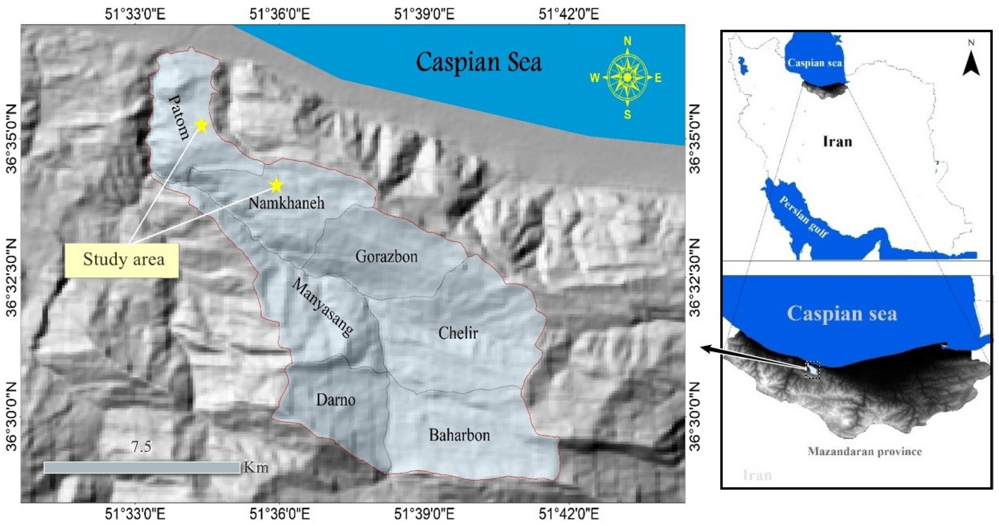
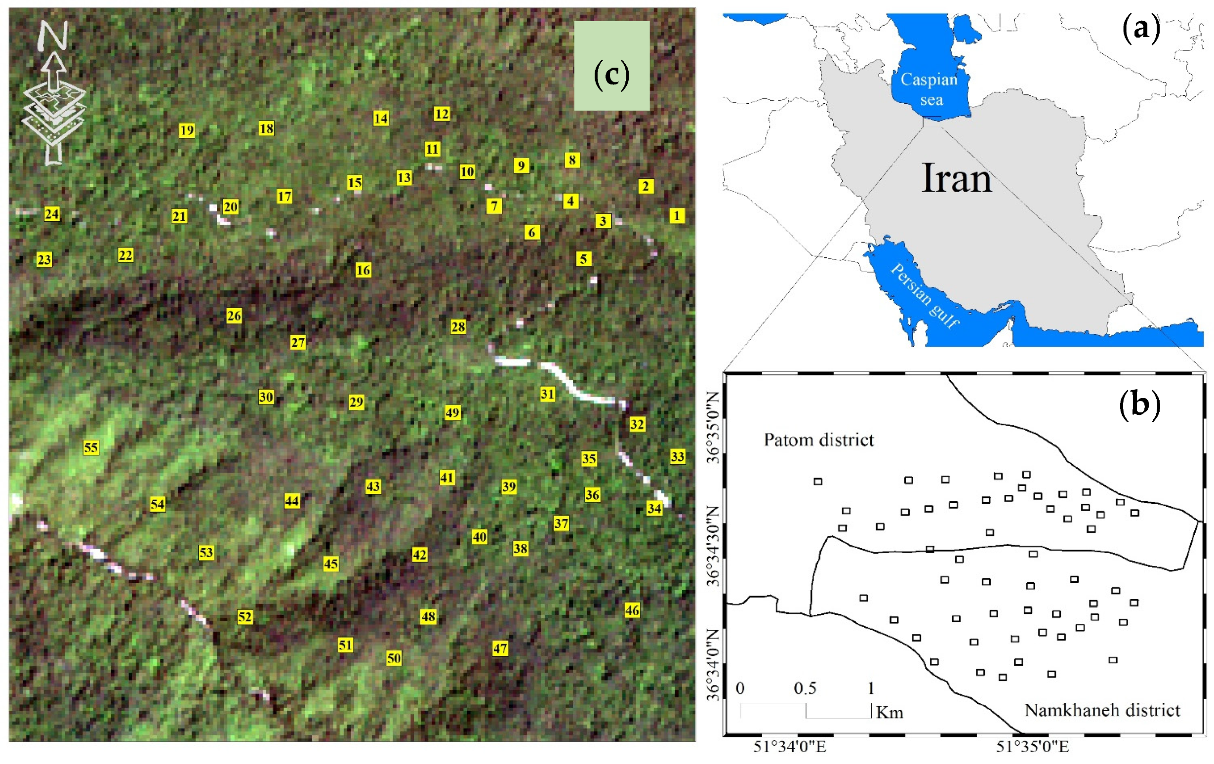
2.1. Study Site
2.2. Remote Sensed Data and Data Preprocessing
2.3. In Situ Measurements
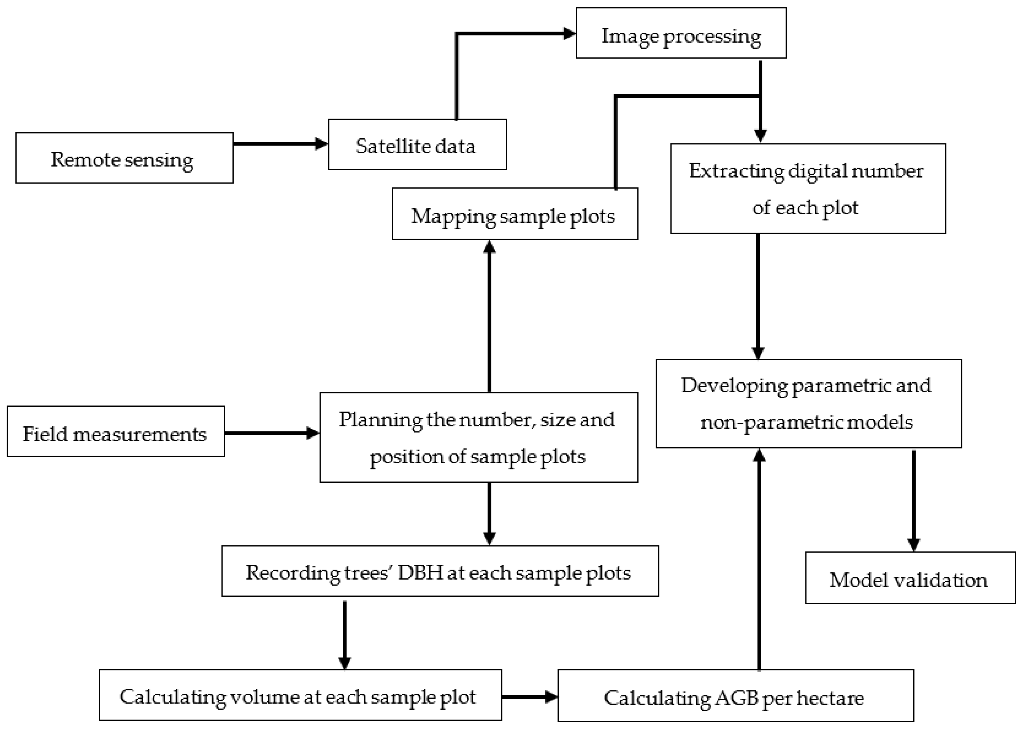
2.4. Methods
2.5. Statistical Analysis and Modeling Performance
3. Results
4. Discussion
5. Conclusions
Author Contributions
Funding
Institutional Review Board Statement
Informed Consent Statement
Data Availability Statement
Acknowledgments
Conflicts of Interest
Appendix A


| Plot No. | Number of Trees | Mean Value of DBH (cm) | Volume (m3/ha) | AGB (t/ha) |
|---|---|---|---|---|
| 1 | 36 | 39 | 326 | 221 |
| 2 | 46 | 41 | 439 | 298 |
| 3 | 46 | 41 | 399 | 271 |
| 4 | 48 | 39 | 463 | 315 |
| 5 | 57 | 37 | 316 | 215 |
| 6 | 70 | 32 | 463 | 315 |
| 7 | 45 | 35 | 292 | 198 |
| 8 | 56 | 30 | 420 | 286 |
| 9 | 88 | 30 | 353 | 240 |
| 10 | 32 | 50 | 305 | 208 |
| 11 | 30 | 35 | 390 | 266 |
| 12 | 42 | 30 | 236 | 160 |
| 13 | 60 | 22 | 174 | 118 |
| 14 | 97 | 20 | 366 | 249 |
| 15 | 88 | 20 | 190 | 129 |
| 16 | 94 | 24 | 273 | 185 |
| 17 | 87 | 30 | 284 | 193 |
| 18 | 60 | 27 | 240 | 163 |
| 19 | 61 | 26 | 229 | 155 |
| 20 | 95 | 23 | 260 | 177 |
| 21 | 81 | 23 | 188 | 128 |
| 22 | 92 | 26 | 224 | 152 |
| 23 | 72 | 26 | 337 | 229 |
| 24 | 62 | 35 | 183 | 124 |
| 25 | 52 | 27 | 234 | 159 |
| 26 | 61 | 32 | 403 | 274 |
| 27 | 42 | 46 | 385 | 262 |
| 28 | 26 | 44 | 304 | 207 |
| 29 | 32 | 53 | 184 | 125 |
| 30 | 29 | 41 | 234 | 159 |
| 31 | 36 | 31 | 470 | 320 |
| 32 | 30 | 36 | 295 | 201 |
| 33 | 40 | 33 | 428 | 291 |
| 34 | 40 | 44 | 338 | 230 |
| 35 | 27 | 40 | 261 | 178 |
| 36 | 45 | 34 | 338 | 230 |
| 37 | 38 | 32 | 189 | 128 |
| 38 | 48 | 32 | 240 | 163 |
| 39 | 55 | 38 | 189 | 128 |
| 40 | 35 | 28 | 461 | 314 |
| 41 | 50 | 42 | 358 | 244 |
| 42 | 34 | 30 | 368 | 250 |
| 43 | 29 | 40 | 272 | 185 |
| 44 | 36 | 34 | 276 | 188 |
| 45 | 66 | 47 | 304 | 207 |
| 46 | 28 | 34 | 452 | 307 |
| 47 | 57 | 41 | 338 | 230 |
| 48 | 29 | 36 | 307 | 209 |
| 49 | 45 | 34 | 218 | 148 |
| 50 | 50 | 43 | 319 | 217 |
| 51 | 49 | 43 | 344 | 234 |
| 52 | 47 | 31 | 278 | 189 |
| 53 | 55 | 31 | 207 | 141 |
| 54 | 75 | 29 | 175 | 119 |
| 55 | 61 | 21 | 446 | 303 |
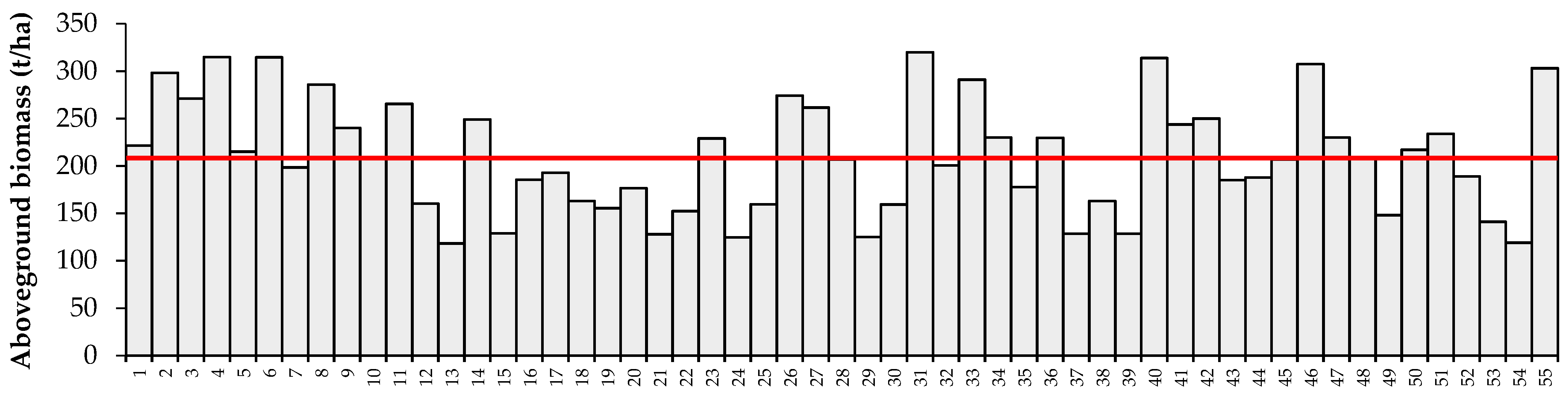
| Minimum | 26 | 20 | 174 | 118 |
| Maximum | 97 | 53 | 470 | 320 |
| Mean | 52.58 | 33.96 | 308.45 | 209.73 |
| Variance | 397.62 | 59.85 | 7752.70 | 3598.24 |
| Standard Deviation | 19.94 | 7.74 | 88.05 | 59.99 |
References
- Phat, N.K.; Knorr, W.; Kim, S. Appropriate measures for conservation of terrestrial carbon stocks—Analysis of trends of forest management in Southeast Asia. For. Ecol. Manag. 2004, 191, 283–299. [Google Scholar] [CrossRef]
- Nalaka, G.D.A.; Sivanathawerl, T.; Iqbal, M.C.M. Scaling aboveground biomass from small diameter trees. Trop. Agric. Res. 2013, 24, 150–162. [Google Scholar]
- Darkwah, S.O.; Scoville, M.D.; Wang, L.K. Geographic information systems and remote sensing applications in environmental and water resources. In Integrated Natural Resources Management; Springer: Cham, Switzerland, 2021; pp. 197–236. [Google Scholar]
- Holmgren, J.; Joyce, S.; Nilsson, M.; Olsson, H. Estimating stem volume and basal area in forest compartments by combining satellite image data with field data. Scand. J. For. Res. 2000, 15, 103–111. [Google Scholar] [CrossRef]
- Agata, H.; Aneta, L.; Dariusz, Z.; Krzysztof, S.; Marek, L.; Christiane, S.; Carsten, P. Forest aboveground biomass estimation using a combination of Sentinel-1 and Sentinel-2 Data. In Proceedings of the IGARSS 2018—2018 IEEE International Geoscience and Remote Sensing Symposium, Valencia, Spain, 22–27 July 2018; pp. 9026–9029. [Google Scholar]
- Aranha, J.; Enes, T.; Calvão, A.; Viana, H. Shrub biomass estimates in former burnt areas using Sentinel 2 images processing and classification. Forests 2020, 11, 555. [Google Scholar] [CrossRef]
- Chen, L.; Ren, C.; Zhang, B.; Wang, Z.; Xi, Y. Estimation of forest above-ground biomass by geographically weighted regression and machine learning with sentinel imagery. Forests 2018, 9, 582. [Google Scholar] [CrossRef]
- Heiskanen, J. Estimating aboveground tree biomass and leaf area index in a mountain birch forest using ASTER satellite data. Int. J. Remote Sens. 2006, 27, 1135–1158. [Google Scholar] [CrossRef]
- Li, L.; Zhou, X.; Chen, L.; Chen, L.; Zhang, Y.; Liu, Y. Estimating urban vegetation biomass from Sentinel-2A image data. Forests 2020, 11, 125. [Google Scholar] [CrossRef]
- Mohammadi, J. Investigating Estimation Some Quantitative Characteristics for Presentation Location Models Using Landsat ETM+ Satellite Data. Master’s Thesis, Gorgan University of Agriculture and Natural Sciences, Gorgan, Iran, 2007. [Google Scholar]
- Moradi, F.; Darvishsefat, A.A.; Namiranian, M.; Ronoud, G. Investigating the capability of Landsat 8 OLI data for estimation of aboveground woody biomass of common hornbeam (Carpinus betulus L.) stands in Khyroud Forest. Iran. J. For. Pop. Res. 2018, 26, 406–420. [Google Scholar]
- Safari, A.; Sohrabi, H. Ability of Landsat-8 OLI derived texture metrics in estimating aboveground carbon stocks of coppice Oak Forests. In Proceedings of the International Archives of the Photogrammetry, Remote Sensing and Spatial Information Sciences, Prague, Czech Republic, 12–19 July 2016; Volume 41. [Google Scholar]
- Zheng, D.; Rademacher, J.; Chen, J.; Crow, T.; Bresee, M.; Le Moine, J.; Ryu, S.R. Estimating aboveground biomass using Landsat 7 ETM+ data across a managed landscape in northern Wisconsin, USA. Remote Sens. Environ. 2004, 93, 402–411. [Google Scholar] [CrossRef]
- Gao, L.; Zhang, X. Above-Ground Biomass Estimation of Plantation with Complex Forest Stand Structure Using Multiple Features from Airborne Laser Scanning Point Cloud Data. Forests 2021, 12, 1713. [Google Scholar] [CrossRef]
- Wu, C.; Tao, H.; Zhai, M.; Lin, Y.; Wang, K.; Deng, J.; Shen, A.; Gan, M.; Li, J.; Yang, H. Using nonparametric modeling approaches and remote sensing imagery to estimate ecological welfare forest biomass. J. For. Res. 2018, 29, 151–161. [Google Scholar] [CrossRef]
- Roy, S.; Mudi, S.; Das, P.; Ghosh, S.; Shit, P.K.; Bhunia, G.S.; Kim, J. Estimating Above Ground Biomass (AGB) and Tree Density using Sentinel-1 Data. In Spatial Modeling in Forest Resources Management; Springer: Cham, Switzerland, 2021; pp. 259–280. [Google Scholar]
- Kumar, L.; Mutanga, O. Remote sensing of above-ground biomass. Remote Sens. 2017, 9, 935. [Google Scholar] [CrossRef]
- Sullivan, M.J.; Lewis, S.L.; Hubau, W.; Qie, L.; Baker, T.R.; Banin, L.F.; Chave, J.; Cuni-Sanchez, A.; Feldpausch, T.R.; Lopez-Gonzalez, G.; et al. Field methods for sampling tree height for tropical forest biomass estimation. Methods Ecol. Evol. 2018, 9, 1179–1189. [Google Scholar] [CrossRef] [PubMed]
- Gao, Y.; Lu, D.; Li, G.; Wang, G.; Chen, Q.; Liu, L.; Li, D. Comparative Analysis of modeling algorithms for forest aboveground biomass estimation in a Subtropical region. Remote Sens. 2018, 10, 627. [Google Scholar] [CrossRef]
- Foody, G.M.; Cutler, M.E.; McMorrow, J.; Pelz, D.; Tangki, H.; Boyd, D.S.; Douglas, I. Mapping the biomass of bornean tropical rain forest from remotely sensed data. Glob. Ecol. Biogeogr. 2001, 10, 379–387. [Google Scholar] [CrossRef]
- Chirici, G.; Barbati, A.; Corona, P.; Marchetti, M.; Travaglini, D.; Maselli, F.; Bertini, R. Non-parametric and parametric methods using satellite images for estimating growing stock volume in alpine and Mediterranean forest ecosystems. Remote Sens. Environ. 2008, 112, 2686–2700. [Google Scholar] [CrossRef]
- Gu, H.; Dai, L.; Wu, G.; Xu, D.; Wang, S.; Wang, H. Estimation of forest volumes by integrating Landsat TM imagery and forest inventory data. Sci. China Ser. E Technol. Sci. 2006, 49, 54–62. [Google Scholar] [CrossRef]
- McRoberts, R.E.; Tomppo, E.O. Remote sensing support for national forest inventories. Remote Sens. Environ. 2007, 110, 412–419. [Google Scholar] [CrossRef]
- Eskelson, B.N.; Barrett, T.M.; Temesgen, H. Imputing mean annual change to estimate current forest attributes. Silva Fenn. 2009, 43, 649–658. [Google Scholar] [CrossRef][Green Version]
- Hudak, A.T.; Strand, E.K.; Vierling, L.A.; Byrne, J.C.; Eitel, J.U.H.; Martinuzzi, S.; Falkowski, M.J. Quantifying aboveground forest carbon pools and fluxes from repeat LiDAR surveys. Remote Sens. Environ. 2012, 123, 25–40. [Google Scholar] [CrossRef]
- Rajab Pourrahmati, M.; Baghdadi, N.; Darvishsefat, A.; Namiranian, M.; Gond, V.; Bailly, J.S.; Zargham, N. Mapping Lorey’s height over Hyrcanian forests of Iran using synergy of ICESat/GLAS and optical images. Eur. J. Remote Sens. 2018, 51, 100–115. [Google Scholar] [CrossRef]
- Breiman, L. Bagging predictors. Mach. Learn. 1996, 24, 123–140. [Google Scholar] [CrossRef]
- Breiman, L. Random forests. Mach. Learn. 2001, 45, 5–32. [Google Scholar] [CrossRef]
- Shahrokhzadeh, U.; Sohrabi, H.; Copenheaver, C.A. Aboveground biomass and leaf area equations for three common tree species of Hyrcanian temperate forests in northern Iran. Botany 2015, 93, 663–670. [Google Scholar] [CrossRef]
- Muukkonen, P.; Heiskanen, J. Estimating biomass for boreal forests using ASTER satellite data combined with standwise forest inventory data. Remote Sens. Environ. 2005, 99, 434–447. [Google Scholar] [CrossRef]
- Yadav, B.K.; Nandy, S. Mapping aboveground woody biomass using forest inventory, remote sensing and geostatistical techniques. Environ. Monit. Assess. 2015, 187, 308. [Google Scholar] [CrossRef]
- Lu, D.; Chen, Q.; Wang, G.; Liu, L.; Li, G.; Moran, E. A survey of remote sensing-based aboveground biomass estimation methods in forest ecosystems. Int. J. Dig. Earth 2016, 9, 63–105. [Google Scholar] [CrossRef]
- Ronoud, G.; Darvishsefat, A. Estimating aboveground woody biomass of Fagus orientalis stands in Hyrcanian forest of Iran using Landsat 5 satellite data (Case study: Khyroud Forest). Geogr. Space 2018, 17, 117–129. [Google Scholar]
- Forkuor, G.; Zoungrana, J.B.B.; Dimobe, K.; Ouattara, B.; Vadrevu, K.P.; Tondoh, J.E. Above-ground biomass mapping in West African dryland forest using Sentinel-1 and 2 datasets-A case study. Remote Sens. Environ. 2020, 236, 111496. [Google Scholar] [CrossRef]
- Laurin, G.V.; Balling, J.; Corona, P.; Mattioli, W.; Papale, D.; Puletti, N.; Rizzo, M.; Truckenbrodt, J.; Urban, M. Above-ground biomass prediction by Sentinel-1 multitemporal data in central Italy with integration of ALOS2 and Sentinel-2 data. J. Appl. Remote Sens. 2018, 12, 016008. [Google Scholar] [CrossRef]
- Theofanous, N.; Chrysafis, I.; Mallinis, G.; Domakinis, C.; Verde, N.; Siahalou, S. Aboveground Biomass Estimation in Short Rotation Forest Plantations in Northern Greece Using ESA’s Sentinel Medium-High Resolution Multispectral and Radar Imaging Missions. Forests 2021, 12, 902. [Google Scholar] [CrossRef]
- Castillo, J.A.A.; Apan, A.A.; Maraseni, T.N.; Salmo, S.G., III. Estimation and mapping of above-ground biomass of mangrove forests and their replacement land uses in the Philippines using Sentinel imagery. ISPRS J. Photogram. Remote Sens. 2017, 134, 70–85. [Google Scholar] [CrossRef]
- Chen, L.; Wang, Y.; Ren, C.; Zhang, B.; Wang, Z. Assessment of multi-wavelength SAR and multispectral instrument data for forest aboveground biomass mapping using random forest kriging. For. Ecol. Manag. 2019, 447, 12–25. [Google Scholar] [CrossRef]
- Ghosh, S.M.; Behera, M.D. Aboveground biomass estimation using multi-sensor data synergy and machine learning algorithms in a dense tropical forest. Appl. Geogr. 2018, 96, 29–40. [Google Scholar] [CrossRef]
- Hernández-Stefanoni, J.L.; Castillo-Santiago, M.Á.; Mas, J.F.; Wheeler, C.E.; Andres-Mauricio, J.; Tun-Dzul, F.; George-Chacón, S.P.; Reyes-Palomeque, G.; Castellanos-Basto, B.; Vaca, R.; et al. Improving aboveground biomass maps of tropical dry forests by integrating LiDAR, ALOS PALSAR, climate and field data. Carbon Balance Manag. 2020, 15, 15. [Google Scholar] [CrossRef]
- Khan, M.R.; Khan, I.A.; Baig, M.H.A.; Liu, Z.J.; Ashraf, M.I. Exploring the potential of Sentinel-2A satellite data for aboveground biomass estimation in fragmented Himalayan subtropical pine forest. J. Mt. Sci. 2020, 17, 2880–2896. [Google Scholar] [CrossRef]
- Pandit, S.; Tsuyuki, S.; Dube, T. Estimating above-ground biomass in sub-tropical buffer zone community forests, Nepal, using Sentinel 2 data. Remote Sens. 2018, 10, 601. [Google Scholar] [CrossRef]
- Majasalmi, T.; Rautiainen, M. The potential of Sentinel-2 data for estimating biophysical variables in a boreal forest: A simulation study. Remote Sens. Lett. 2016, 7, 427–436. [Google Scholar] [CrossRef]
- Puliti, S.; Hauglin, M.; Breidenbach, J.; Montesano, P.; Neigh, C.S.R.; Rahlf, J.; Solberg, S.; Klingenberg, T.F.; Astrup, R. Modelling above-ground biomass stock over Norway using national forest inventory data with ArcticDEM and Sentinel-2 data. Remote Sens. Environ. 2020, 236, 111501. [Google Scholar] [CrossRef]
- Wang, J.; Xiao, X.; Bajgain, R.; Starks, P.; Steiner, J.; Doughty, R.B.; Chang, Q. Estimating leaf area index and aboveground biomass of grazing pastures using Sentinel-1, Sentinel-2 and Landsat images. ISPRS J. Photogram. Remote Sens. 2019, 154, 189–201. [Google Scholar] [CrossRef]
- Chrysafis, I.; Mallinis, G.; Siachalou, S.; Patias, P. Assessing the relationships between growing stock volume and Sentinel-2 imagery in a Mediterranean forest ecosystem. Remote Sens. Lett. 2017, 8, 508–517. [Google Scholar] [CrossRef]
- Nuthammachot, N.; Phairuang, W.; Wicaksono, P.; Sayektiningsih, T. Estimating aboveground biomass on private forest using Sentinel-2 imagery. J. Sens. 2018, 2018, 6745629. [Google Scholar]
- Vafaei, S.; Soosani, J.; Adeli, K.; Fadaei, H.; Naghavi, H.; Pham, T.D.; Tien Bui, D. Improving accuracy estimation of Forest Aboveground Biomass based on incorporation of ALOS-2 PALSAR-2 and Sentinel-2A imagery and machine learning: A case study of the Hyrcanian forest area (Iran). Remote Sens. 2018, 10, 172. [Google Scholar] [CrossRef]
- Wernick, I.K.; Ciais, P.; Fridman, J.; Högberg, P.; Korhonen, K.T.; Nordin, A.; Kauppi, P.E. Quantifying forest change in the European Union. Nature 2021, 592, E13–E14. [Google Scholar] [CrossRef]
- Food and Agriculture Organization (FAO). Global Forest Resources Assessment (FRA); Report, Iran (Islamic Republic of); FAO: Rome, Italy, 2020. [Google Scholar]
- Deljouei, A.; Sadeghi, S.M.M.; Abdi, E.; Bernhardt-Römermann, M.; Pascoe, E.L.; Marcantonio, M. The impact of road disturbance on vegetation and soil properties in a beech stand, Hyrcanian forest. Eur. J. For. Res. 2018, 137, 759–770. [Google Scholar] [CrossRef]
- Rahbarisisakht, S.; Moayeri, M.H.; Hayati, E.; Sadeghi, S.M.M.; Kepfer-Rojas, S.; Pahlavani, M.H.; Kappel Schmidt, I.; Borz, S.A. Changes in Soil’s Chemical and Biochemical Properties Induced by Road Geometry in the Hyrcanian Temperate Forests. Forests 2021, 12, 1805. [Google Scholar] [CrossRef]
- Abbasian, P.; Attarod, P.; Sadeghi, S.M.M.; Van Stan, J.T.; Hojjati, S.M. Throughfall nutrients in a degraded indigenous Fagus orientalis forest and a Picea abies plantation in the of North of Iran. For. Syst. 2015, 24, 1. [Google Scholar] [CrossRef]
- Marvie-Mohadjer, M.R. Silviculture, 5th ed.; University of Tehran Press: Tehran, Iran, 2019; p. 418. [Google Scholar]
- Haghshenas, M.; Mohadjer, M.R.M.; Attarod, P.; Pourtahmasi, K.; Feldhaus, J.; Sadeghi, S.M.M. Climate effect on tree-ring widths of Fagus orientalis in the Caspian forests, northern Iran. For. Sci. Technol. 2016, 12, 176–182. [Google Scholar]
- Lu, D.; Batistella, M.; Moran, E. Satellite estimation of aboveground biomass and impacts of forest stand structure. Photogramm. Eng. Remote Sens. 2005, 71, 967–974. [Google Scholar] [CrossRef]
- Drusch, M.; Del Bello, U.; Carlier, S.; Colin, O.; Fernandez, V.; Gascon, F.; Hoersch, B.; Isola, C.; Laberinti, P.; Martimort, P.; et al. Sentinel-2: ESA’s optical high-resolution mission for GMES operational services. Remote Sens. Environ. 2012, 120, 25–36. [Google Scholar] [CrossRef]
- Crippen, R.E. Calculating the vegetation index faster. Remote Sens. Environ. 1990, 34, 71–73. [Google Scholar] [CrossRef]
- Frampton, W.J.; Dash, J.; Watmough, G.; Milton, E.J. Evaluating the capabilities of Sentinel-2 for quantitative estimation of biophysical variables in vegetation. ISPRS J. Photogram. Remote Sens. 2013, 82, 83–92. [Google Scholar] [CrossRef]
- Pinty, B.; Verstraete, M. GEMI: A non-linear index to monitor global vegetation from satellites. Vegetatio 1992, 101, 15–20. [Google Scholar] [CrossRef]
- Gitelson, A.A.; Kaufman, Y.J.; Merzlyak, M.N. Use of a green channel in remote sensing of global vegetation from EOS-MODIS. Remote Sens. Environ. 1996, 58, 289. [Google Scholar] [CrossRef]
- Rouse, J.W.; Haas, R.H.; Schell, J.A.; Deering, D.W. Monitoring vegetation systems in the Great Plains with ERTS. NASA Spec. Publ. 1974, 351, 309. [Google Scholar]
- Tucker, C.J.; Elgin, J., Jr.; McMurtrey, J., III; Fan, C. Monitoring corn and soybean crop development with hand-held radiometer spectral data. Remote Sens. Environ. 1979, 8, 237–248. [Google Scholar] [CrossRef]
- Roujean, J.L.; Breon, F.M. Estimating PAR absorbed by vegetation from bidirectional reflectance measurements. Remote Sens. Environ. 1995, 51, 375–384. [Google Scholar] [CrossRef]
- Jordan, C.F. Derivation of leaf-area index from quality of light on the forest floor. Ecology 1969, 50, 663–666. [Google Scholar] [CrossRef]
- Brown, S. Estimating Biomass and Biomass Change of Tropical Forests: A Primer; FAO: Rome, Italy, 1997. [Google Scholar]
- Safdari, V.; Ahmed, M.; Palmer, J.; Baig, M.B. Identification of Iranian commercial wood with hand lens. Pak. J. Bot. 2008, 40, 1851–1864. [Google Scholar]
- Tomppo, E.; Halme, M. Using coarse scale forest variables as ancillary information and weighting of variables in k-NN estimation: A genetic algorithm approach. Remote Sens. Environ. 2004, 92, 1–20. [Google Scholar] [CrossRef]
- Tian, X.; Su, Z.; Chen, E.; Li, Z.; van der Tol, C.; Guo, J.; He, Q. Estimation of forest above-ground biomass using multi-parameter remote sensing data over a cold and arid area. Int. J. Appl. Earth Obs. Geoinf. 2012, 14, 160–168. [Google Scholar] [CrossRef]
- Tojal, L.T.; Bastarrika, A.; Barrett, B.; Sanchez Espeso, J.M.; Lopez-Guede, J.M.; Graña, M. Prediction of Aboveground Biomass from Low-Density LiDAR Data: Validation over P. radiata Data from a Region North of Spain. Forests 2019, 10, 819. [Google Scholar] [CrossRef]
- Civco, D.L. Artificial neural networks for land-cover classification and mapping. Int. J. Geogr. Inf. Sci. 1993, 7, 173–186. [Google Scholar] [CrossRef]
- Mas, J. Mapping land use/cover in a tropical coastal area using satellite sensor data, GIS and artificial neural networks. Estuar. Coast. Shelf Sci. 2004, 59, 219–230. [Google Scholar] [CrossRef]
- Cheţa, M.; Marcu, M.V.; Borz, S.A. Effect of training parameters on the ability of artificial neural networks to learn: A Simulation on accelerometer data for task recognition in motormanual felling and processing. Bull. Transilv. Univ. Bras. Ser. II For. Wood Ind. Agric. Food Eng. 2020, 13, 19–36. [Google Scholar] [CrossRef]
- Zealand, C.M.; Burn, D.H.; Simonovic, S.P. Short term streamflow forecasting using artificial neural networks. J. Hydrol. 1999, 214, 32–48. [Google Scholar] [CrossRef]
- Tiryaki, S.; Aydın, A. An artificial neural network model for predicting compression strength of heat treated woods and comparison with a multiple linear regression model. Constr. Build. Mater. 2014, 62, 102–108. [Google Scholar] [CrossRef]
- Pham, T.D.; Yoshino, K.; Bui, D.T. Biomass estimation of Sonneratia caseolaris (L.) Engler at a coastal area of Hai Phong city (Vietnam) using ALOS-2 PALSAR imagery and GIS-based multi-layer perceptron neural networks. GISci. Remote Sens. 2017, 54, 329–353. [Google Scholar] [CrossRef]
- Bui, D.T.; Tuan, T.A.; Klempe, H.; Pradhan, B.; Revhaug, I. Spatial prediction models for shallow landslide hazards: A comparative assessment of the efficacy of support vector machines, artificial neural networks, kernel logistic regression, and logistic model tree. Landslides 2016, 13, 361–378. [Google Scholar]
- Shataee, S.; Kalbi, S.; Fallah, A.; Pelz, D. Forest attribute imputation using machine-learning methods and ASTER data: Comparison of k-NN, SVR and random forest regression algorithms. Int. J. Remote Sens. 2012, 33, 6254–6280. [Google Scholar] [CrossRef]
- Statistica. Electronic Text Book; Stat Soft Inc.: Tulsa, OK, USA, 2010; Available online: www.Statsoft.com (accessed on 22 October 2020).
- Franco-Lopez, H.; Ek, A.R.; Bauer, M.E. Estimation and mapping of forest stand density, volume, and cover type using the k-nearest neighbors method. Remote Sens. Environ. 2001, 77, 251–274. [Google Scholar] [CrossRef]
- Reese, H.; Nilsson, M.; Sandström, P.; Olsson, H. Applications using estimates of forest parameters derived from satellite and forest inventory data. Comput. Electron. Agric. 2002, 37, 37–55. [Google Scholar] [CrossRef]
- Sironen, S.; Kangas, A.; Maltamo, M. Comparison of different non-parametric growth imputation methods in the presence of correlated observations. Forestry 2010, 83, 39–51. [Google Scholar] [CrossRef]
- Pelletier, C.; Valero, S.; Inglada, J.; Champion, N.; Dedieu, G. Assessing the robustness of Random Forests to map land cover with high resolution satellite image time series over large areas. Remote Sens. Environ. 2016, 187, 156–168. [Google Scholar] [CrossRef]
- Friedman, J.H. The Elements of Statistical Learning: Data Mining, Inference, and Prediction; Springer: New York, NY, USA, 2017. [Google Scholar]
- Gislason, P.O.; Benediktsson, J.A.; Sveinsson, J.R. Random forests for land cover classification. Pattern Recognit. Lett. 2006, 27, 294–300. [Google Scholar] [CrossRef]
- Rodriguez-Galiano, V.F.; Ghimire, B.; Rogan, J.; Chica-Olmo, M.; Rigol-Sanchez, J.P. An assessment of the effectiveness of a random forest classifier for land-cover classification. ISPRS J. Photogramm. Remote Sens. 2012, 67, 93–104. [Google Scholar] [CrossRef]
- Stevens, F.R.; Gaughan, A.E.; Linard, C.; Tatem, A.J. Disaggregating census data for population mapping using random forests with remotely-sensed and ancillary data. PLoS ONE 2015, 10, e0107042. [Google Scholar] [CrossRef]
- Tavasoli, N.; Arefi, H. Comparison of capability of SAR and optical data in mapping forest above ground biomass based on machine learning. Environ. Sci. Proc. 2020, 5, 13. [Google Scholar] [CrossRef]
- Baloloy, A.B.; Blanco, A.C.; Candido, C.G.; Argamosa, R.J.L.; Dumalag, J.B.L.C.; Dimapilis, L.L.C.; Paringit, E.C. Estimation of mangrove forest aboveground biomass using multispectral bands, vegetation indices and biophysical variables derived from optical satellite imageries: Rapideye, planetscope and sentinel-2. ISPRS Ann. Photogramm. Remote Sens. Spat. Inf. Sci. 2018, 4, 29–36. [Google Scholar] [CrossRef]
- Lu, D. Aboveground biomass estimation using Landsat TM data in the Brazilian Amazon. Int. J. Remote Sens. 2005, 26, 2509–2525. [Google Scholar] [CrossRef]
- Roy, P.; Ravan, S.A. Biomass estimation using satellite remote sensing data—An investigation on possible approaches for natural forest. J. Biosci. 1996, 21, 535–561. [Google Scholar] [CrossRef]
- Liu, Y.; Gong, W.; Xing, Y.; Hu, X.; Gong, J. Estimation of the forest stand mean height and aboveground biomass in Northeast China using SAR Sentinel-1B, multispectral Sentinel-2A, and DEM imagery. ISPRS J. Photogramm. Remote Sens. 2019, 151, 277–289. [Google Scholar] [CrossRef]
- Rudnicki, M.; Silins, U.; Lieffers, V.J. Crown cover is correlated with relative density, tree slenderness, and tree height in lodgepole pine. For. Sci. 2004, 50, 356–363. [Google Scholar]
- Butera, M.K. A correlation and regression analysis of percent canopy closure versus TMS spectral response for selected forest sites in the San Juan National Forest, Colorado. IEEE Trans. Geosci. Remote Sens. 1986, 1, 122–129. [Google Scholar] [CrossRef]
- Sadeghi, S.M.M.; Van Stan, J.T., II; Pypker, T.G.; Friesen, J. Canopy hydrometeorological dynamics across a chronosequence of a globally invasive species, Ailanthus altissima (Mill., tree of heaven). Agric. For. Meteorol. 2017, 240, 10–17. [Google Scholar] [CrossRef]
- Khorrami, R.; Darvishsefat, A.; Namiranian, M. Investigation on the capability of Landsat7 ETM+ data for standing volume estimation of beech stands (Case study: Sangdeh forests). Iran. J. Nat. Res. 2008, 60, 1281–1289. [Google Scholar]
- Tóth, T.; Schaap, M.G.; Molnár, Z. Utilization of soil-plant interrelations through the use of multiple regression and artificial neural network in order to predict soil properties in Hungarian solonetzic grasslands. Cereal Res. Commun. 2008, 36, 1447–1450. [Google Scholar]
- Lu, D. The potential and challenge of remote sensing-based biomass estimation. Int. J. Remote Sens. 2006, 27, 1297–1328. [Google Scholar] [CrossRef]
- Fatehi, P.; Damm, A.; Schweiger, A.K.; Schaepman, M.E.; Kneubühler, M. Mapping alpine aboveground biomass from imaging spectrometer data: A Comparison of two approaches. IEEE J. Sel. Top. Appl. Earth Obs. Remote Sens. 2015, 8, 3123–3139. [Google Scholar] [CrossRef]
- Kellndorfer, J.; Walker, W.; LaPoint, E.; Kirsch, K.; Bishop, J.; Fiske, G. Statistical fusion of Lidar, InSAR, and optical remote sensing data for forest stand height characterization: A regional-scale method based on LVIS, SRTM, Landsat ETM+, and ancillary data sets. J. Geophys. Res. Biogeosci. 2010, 115, G00E08. [Google Scholar] [CrossRef]
- Ji, L.; Wylie, B.K.; Nossov, D.R.; Peterson, B.; Waldrop, M.P.; McFarland, J.W.; Rover, J.; Hollingsworth, T.N. Estimating aboveground biomass in interior Alaska with Landsat data and field measurements. Int. J. Appl. Earth Obs. Geoinf. 2012, 18, 451–461. [Google Scholar] [CrossRef]
- Chen, Y.; Li, L.; Lu, D.; Li, D. Exploring bamboo forest aboveground biomass estimation using Sentinel-2 data. Remote Sens. 2019, 11, 7. [Google Scholar] [CrossRef]
- Jiang, X.; Li, G.; Lu, D.; Moran, E.; Batistella, M. Modeling Forest Aboveground Carbon Density in the Brazilian Amazon with Integration of MODIS and Airborne LiDAR Data. Remote Sens. 2020, 12, 3330. [Google Scholar] [CrossRef]
- Persson, H.J.; Jonzén, J.; Nilsson, M. Combining TanDEM-X and Sentinel-2 for large-area species-wise prediction of forest biomass and volume. Int. J. Appl. Earth Obs. Geoinf. 2021, 96, 102275. [Google Scholar] [CrossRef]
- Ronoud, G.; Fatehi, P.; Darvishsefat, A.A.; Tomppo, E.; Praks, J.; Schaepman, M.E. Multi-Sensor Aboveground Biomass Estimation in the Broadleaved Hyrcanian Forest of Iran. Can. J. Remote Sens. 2021, 47, 818–834. [Google Scholar] [CrossRef]


| Index | Equation | Reference |
|---|---|---|
| Infrared Percentage Vegetation Index (IPVI) | NIR 1/(NIR + RED 2) | [58] |
| Inverted Red-Edge Chlorophyll Index (IRECI) | (NIR − RED)/(RED/RED) | [59] |
| Global Environment Monitoring Index (GEMI) | n 3 × (1 − 0.25 × n) − (RED − 0.125)/(1 − RED) | [60] |
| Green Normalized Difference Vegetation Index (GNDVI) | (NIR − GREEN 4)/(NIR + GREEN) | [61] |
| Normalized Difference Vegetation Index (NDVI) | (NIR − RED)/(NIR + RED) | [62] |
| Difference Vegetation Index (DVI) | NIR − RED | [63] |
| Pigment Specific Simple Ratio (PSSRA) | NIR/RED | [64] |
| Ratio Vegetation Index (RVI) | NIR/RED | [65] |
| Variable | r | Variable | r |
|---|---|---|---|
| B2 | −0.519 ** | IPVI | −0.506 ** |
| B3 | −0.541 ** | IRECI | −0.567 ** |
| B4 | −0.580 ** | GEMI | −0.666 ** |
| B5 | −0.515 ** | PC1 1 | −0.686 ** |
| B6 | −0.723 ** | GNDVI | −0.322 ** |
| B7 | −0.682 ** | NDVI | −0.506 ** |
| B8 | −0.691 ** | DVI | −0.682 ** |
| B8a | −0.674 ** | PSSRA | −0.425 ** |
| B11 | −0.716 ** | RVI | −0.510 ** |
| B12 | −0.594 ** |
| Regression Method | SEE | R2 | R2adj | %RMSE | Variable |
|---|---|---|---|---|---|
| Multiple | 40.35 | 0.757 | 0.588 | 29.72 | All variables |
| Stepwise | 42.89 | 0.547 | 0.535 | 30.99 | B6 |
| Backward | 35.73 | 0.722 | 0.650 | 24.72 | B2, B4, B5, B6, B7, B11, PCA, GNDVI, NDVI, PSSRA, IRECI, DVI |
| Range of k | Distance Metric | R2 | %RMSE | The Optimal k Value |
|---|---|---|---|---|
| 1–40 | Euclidean | 0.67 | 23.90 | 27 |
| 1–40 | Squared Euclidean | 0.72 | 22.94 | 29 |
| 1–40 | Manhattan | 0.73 | 21.85 | 25 |
| 1–40 | Chebychev | 0.67 | 23.87 | 24 |
| AGB Model | Training Dataset | Validation | ||
|---|---|---|---|---|
| R2 | %RMSE | R2 | %RMSE | |
| MLP NN | 0.89 | 8.79 | 0.65 | 19.93 |
| RF | 0.69 | 19.52 | 0.60 | 22.55 |
Publisher’s Note: MDPI stays neutral with regard to jurisdictional claims in published maps and institutional affiliations. |
© 2022 by the authors. Licensee MDPI, Basel, Switzerland. This article is an open access article distributed under the terms and conditions of the Creative Commons Attribution (CC BY) license (https://creativecommons.org/licenses/by/4.0/).
Share and Cite
Moradi, F.; Darvishsefat, A.A.; Pourrahmati, M.R.; Deljouei, A.; Borz, S.A. Estimating Aboveground Biomass in Dense Hyrcanian Forests by the Use of Sentinel-2 Data. Forests 2022, 13, 104. https://doi.org/10.3390/f13010104
Moradi F, Darvishsefat AA, Pourrahmati MR, Deljouei A, Borz SA. Estimating Aboveground Biomass in Dense Hyrcanian Forests by the Use of Sentinel-2 Data. Forests. 2022; 13(1):104. https://doi.org/10.3390/f13010104
Chicago/Turabian StyleMoradi, Fardin, Ali Asghar Darvishsefat, Manizheh Rajab Pourrahmati, Azade Deljouei, and Stelian Alexandru Borz. 2022. "Estimating Aboveground Biomass in Dense Hyrcanian Forests by the Use of Sentinel-2 Data" Forests 13, no. 1: 104. https://doi.org/10.3390/f13010104
APA StyleMoradi, F., Darvishsefat, A. A., Pourrahmati, M. R., Deljouei, A., & Borz, S. A. (2022). Estimating Aboveground Biomass in Dense Hyrcanian Forests by the Use of Sentinel-2 Data. Forests, 13(1), 104. https://doi.org/10.3390/f13010104