Application of a Panel Data Quantile-Regression Model to the Dynamics of Carbon Sequestration in Pinus kesiya var. langbianensis Natural Forests

Abstract

Even though studies on forest carbon storage are relatively mature, dynamic changes in carbon sequestration have been insufficiently researched. Therefore, we used panel data from 81 Pinus kesiya var. langbianensis forest sample plots measured on three occasions to build an ordinary regression model and a quantile-regression model to estimate carbon sequestration over time. In the models, the average carbon reserve of the natural forests was taken as the dependent variable and the average diameter at breast height (DBH), crown density, and altitude as independent variables. The effects of the DBH and crown density on the average carbon storage differed considerably among different age groups and with time, while the effect of altitude had a relatively insignificant influence. Compared with the ordinary model, the quantile-regression model was more accurate in residual and predictive analyses and removed large errors generated by the ordinary model in fitting for young-aged and over-mature forests. We are the first to introduce panel-data-based modeling to forestry research, and it appears to provide a new solution to better grasp change laws for forest carbon sequestration.

1. Introduction

Forests are the largest terrestrial ecosystems and play an important role in the global carbon cycle [1,2,3,4]. Recently, many studies have focused on forest biomass and carbon storage [5,6,7,8,9], and accurate estimation of forest carbon storage has become an important part of global climate change and carbon cycle research [10,11]. The traditional sample inventory method, vorticity correlation method, and model estimation method all have certain limitations for estimating forest carbon storage [12]. With the development of science and technology, the forest carbon storage estimation method based on remote sensing technology is one of the main estimation methods at present [13]. However, data used in these carbon storage studies have been generally collected from different geographical locations. The environment has an effect on them [14]. These data are often not well-correlated or follow spatially non-normal distributions [15]. A large number of spatial models have been applied [9,16,17], such as the GWR (Geographically weighted regression model), GWRK (Geographically weighted regression kriging model) [18], LMM (Linear mixed model), SEM (Spatial error model), and SLM (Spatial lag model), etc.

The methods of these models consider the spatial autocorrelation in the process of spatial data modeling so that better model parameters can be obtained. More importantly, the unbiased estimation of the model’s standard error can improve the statistical test. However, all of the above studies were performed by collecting data from a static cross-section. Furthermore, even over the entire period of study, the same problem may emerge due to constant tree growth and/or changes in forest carbon fixation capacity [19,20,21,22,23].

In traditional modeling, regression results can be used to evaluate and test the mean reversion. Potential correlations between tail data of variables are difficult to capture, and, hence, it is impossible to cover all characteristics of the spatial distribution of forest carbon reserves. Moreover, when the average and variance for different distribution models are the same, results obtained through the mean value regression are unable to reveal their differences.

Quantile regression (QR) is often used to solve the problem, which relies on conditional quantiles of dependent variables to realize the regression of independent variables, expressed as Q(Y|X = x) = x′β(τ). With different quantiles of dependent variables selected, different regression models can be obtained for interpreting the relationship between the dependent and independent variables [24].

Panel data models are a type of model used in modern theoretical econometrics, where data collection comes from many individuals at many time points, forming two-dimensional data (i.e., data in time- and cross-section dimensions) [25,26]. With data volume generally being several or even tens of times greater than one-dimensional data, panel data can contain more information of greater estimation accuracy. Additionally, panel data can be used to remove the problem of multicollinearity, increase the degrees of freedom in estimations, and build and test complicated structural relationships between variables [27].

Because panel data are two dimensional, when they are used in regression, both significant differences among individuals at the same time and for any specific time cross-sections can be accommodated [28]. Such differences can be expressed in different intercepts on the time and cross-section axes. Based on these principles, a panel data quantile-regression model [29] could be built to study the dynamic change of forest carbon reserves.

On this basis, we collected carbon sequestration measurement data from natural forests of Pinus kesiya var. langbianensis to analyze changing trends. Then, in association with forest and topographical factors, we searched for a way to more accurately estimate forest carbon reserves when data were not normally distributed, such as with the occurrence of peaks or fat tails, and the factors influencing the dynamic change of carbon reserves and exploring laws of change. The focus of our research was to discuss whether a panel data model can be applied to solve forest problems.

2. Research Data

2.1. Sample Plot Data

Pinus kesiya var. langbianensis is an evergreen tree in the family Pinaceae, and is a geographical variety of Pinus kesiya Royle ex Gordon. It tends to grow in the sun and can extend its roots deep underground. It prefers high temperature and moisture sites and cannot tolerate cold, drought or barren soil. It is widely distributed in Yunnan provinces, where south subtropical and tropical climates prevail, such as Malipo, Simao, Pu’er, and Jingdong in the south and Luxi in the west. In these areas, at altitudes from 600 to 1700 m, there are broad valleys with low mountains at the periphery of basins, hills, and mountain land on both sides of rivers. The annual average temperature is between 17 and 22 °C, the annual precipitation is more than 1500 mm, and relative humidity is above 80%. Pinus kesiya var. langbianensis has become an important species in Yunnan plantations in recent years because of its rapid growth and extensive uses. In distribution areas and forest stock, it accounts for 11% of Yunnan forests and has enormous economic value, ecological functions, and carbon sequestration benefits.

We used data from three Yunnan forest surveys of 123 permanent sample plots (in the years 2007, 2012, and 2017) where Pinus kesiya var. langbianensis is the dominant species. After the removal of human interference, 81 plots (with the area of 0.08 hectares) are left in each phase. The data covered every Pinus kesiya var. langbianensis distribution area, and the geographic location (GPS coordinates) and origin (artificial or natural) were recorded for each plot. Tree tallying was conducted, and forest stand variables were obtained, including the average DBH (cm), age groups (determined on average age and origin), crown density (ratio of canopy vertical projection area to plot area, no unit), and stock volume (m³ per hectare).

Dem (ASTER GDEM V3) data were also collected to extract terrain characteristics. This includes the altitude (the central point of the sample plot, m), topographic position index (TPI, the average of the central point and the surrounding elevation), terrain ruggedness index (TRI, the average between central elevation minus surrounding elevation), topographic wetness index (TWI, physical indicators of the influence of regional topography on runoff direction and accumulation), and solar radiation (total annual solar radiation, kWh/m²Y).

Three years’ worth (2007, 2012, 2017) of meteorological records were collected from the 28 weather stations in the provinces of Yunnan. Kriging interpolation was used to obtain the temperature and precipitation data from these weather stations for each sample plot in this study at interpolation precision >80%.

Sample plot distributions are shown in Figure 1 and stand statistics in

Table 1. Descriptive statistics of fitted variables used in this study.

Variable	Year	N	Mean	S.D.	Minimum	Maximum
Avg_DBH (cm)	2007	81	15.31	5.83	6.2	28
	2012	81	15.81	5.57	7.6	28
	2017	81	17.20	5.13	3.1	30.1
Crown Density	2007	81	54.22	19.59	22	88
	2012	81	55.52	19.26	22	85
	2017	81	59.24	15.67	22	85
Stock Volume (m3 per hectare)	2007	81	96.85	54.45	2.63	272.99
	2012	81	112.63	54.29	24.86	284.93
	2017	81	125.35	56.55	0.54	297.8
Temp (°C)	2007	81	19.46	0.10	17.52	21.74
	2012	81	27.1	0.10	26.10	28.70
	2017	81	26.2	0.07	25.28	27.78
Precipitation (mm)	2007	81	1399.98	11.26	1213.70	1614.15
	2012	81	1037.76	23.18	788.06	1554.10
	2017	81	1405.97	15.17	1163.18	1779.02
Topographic Position Index (TPI)		81	0.92	0.42	−7.5	11.88
Terrain Ruggedness Index (TRI)		81	9.42	0.47	1.63	20.88
Topographic Wetness Index (TWI)		81	5.49	0.31	0.32	10.69
Solar radiation (kWh/m2Y)		81	1179.86	79.8	29.2	2602.23
Altitude (m)		81	1450	260	930	2220

.

2.2. Biomass and Carbon Content Determination

Pinus kesiya var. langbianensis is concentrated in the southern part of Yunnan provinces, and the growth characteristics will not change. Further, in this paper, due to the short time span, the change of carbon content in the atmosphere caused by human interference has not been considered, only the change of natural carbon sequestration capacity of Pinus kesiya var. Langbianensis was studied in order to fully reflect the environmental characteristics of its distribution and take the conservation of resources into consideration. Therefore, standard trees were collected from north, central, and south counties (Mojiang, Simao and Lancang). So, 128 standard trees of 2013 were selected in this paper to calculate the forest carbon storage of the sample plot.

Table 2. Descriptive statistics of sample trees used in this study.

PLOT	Trees Number	DBH (cm)				H (m)				Age				C (Kg)
		Min.	Max.	Mean	Std.	Min.	Max.	Mean	Std.	Min.	Max.	Mean	Std.	Min.	Max.	Mean	Std.
Mojiang	28	4.4	47	27.6	9.9	6.8	23.9	17.3	3.9	8	39	30	7	1.66	605.61	191.01	155.32
Simao	64	5.9	58.3	22.9	11.9	6.1	27.4	16.7	5.4	14	82	42	18	3.42	1323.4	174.27	223.38
Lancang	36	9.7	51.5	34.5	12.5	8.7	37	24.4	7.5	14	58	43	12	12.01	924.84	352.34	230.4

records their basic statistics. After cutting down a sample tree, the trunk was cut into 1 m long segments, and the trunk’s fresh weight was obtained by adding together the weight of all segments. The crown was separated into three levels, and three to five standard branches were selected from each level to measure the branch’s and leaf’s fresh weight. The roots were totally excavated and classified into three groups (>5 cm, 2–5 cm, and <2 cm) for measuring the fresh weight. Samples that weighed c. 100 g were taken from the trunk, branches, leaves, and roots of three groups of every sample tree and dried at 105 °C until reaching a constant weight. The dry weight was recorded. The biomass of the trunk, branches, leaves, and roots was obtained based on the proportion of the dry weight to the fresh weight. Dried samples of the trunk, branches, leaves, and roots of the three groups were grounded, and c. 50 mg powder samples were analyzed for carbon content using a C/N analysis meter.

Using the Pinus kesiya var. langbianensis biomass model [30], the individual tree biomass in every permanent sample plot was obtained, and sample plot carbon content was calculated by multiplying the biomass by the carbon content. Furthermore, the average carbon reserve of each permanent sample plot was acquired.

Table 3. The basic statistics of carbon storage (ton per hectare).

Variable (t)	Year	N	Mean	S.D.	Minimum	Maximum
C1	2007	81	25.73	15.65	0.74	73.08
C2	2012	81	27.93	15.72	6.74	76.27
C3	2017	81	32.17	15.55	0.15	79.72

includes the basic statistics of the average carbon reserve of every sample plot for each of the three surveys.

3. Research Method

3.1. Method for Selection of Panel Data Model

For the purpose of comparison, an ordinary panel data regression model was built based on data obtained. Ordinary panel data comes in three types: mixed-regression, fixed-effect, and random-effect.

For a panel data:

$$y_{it}=\alpha +X_{it}\beta +{\epsilon }_{it}$$

(1)

where, y is the explained variable, X is the explanatory variable, $\alpha$ is the intercept, $\beta$ is the coefficient, $\epsilon$ is the interference term, i is different individuals, and t is the time.

If there is no significant difference between individuals in terms of time and cross-sections, it is a mixed-regression model, which can be estimated by the ordinary least square (OLS) method. If the model intercepts are different for different sections or time series, the regression parameters can be estimated by adding dummy variables to the model, which is called the fixed-effect model. In the fixed-effect model, individual differences are reflected in that each individual has a specific intercept term. When all individuals have the same intercept term, individual differences are mainly reflected in the setting of a random interference term, which is the random-effect model. The random-effect model requires a generalized least square (GLS) estimation.

Deciding whether to use a fixed-effect model or a mixed-regression model is decided by the result of the F-test. The basic idea of the test is that under the null hypothesis, and the individual effect is not significant, the following relationship should be established:

$$H_0:{\alpha }_1={\alpha }_2=\cdots ={\alpha }_n$$

The F-test can be used to check whether the above hypothesis is true. The F-test is expressed as follow:

$$F=\frac{(R_u^2-R_r^2)/(n-1)}{(1-R_u^2)/(nT-n-T)}~F(n-1,nT-n-K)$$

(2)

where, $R_u^2$ is the sum of squared residuals of the mixed-regression model, $R_r^2$ is the sum of squared residuals of the fixed-effect model, K is the number of explanatory variables.

The F-test results showed that the null hypothesis was rejected, which means that individual effects were present in the model. Whether it is a random- or fixed-effect model can be determined using the Hausman test.

The basic idea is: under the null hypothesis, where α_i is not correlated with other explanatory variables, parameter estimates obtained by OLS estimation of the fixed-effect model and GLS estimation of the random-effect model are unbiased and consistent but the former is not effective. That is, under the null hypothesis, there should be no significant difference between the parameter estimates of the two. Based on this, we can construct statistical tests for the estimation of the two parameters.

Assuming that ${\beta }_{FE}$ and ${\beta }_{RE}$ are OLS estimations of the fixed-effect model and GLS estimations of the random-effect model, respectively, then:

$$Var\left[{\beta }_{FE}-{\beta }_{RE}\right]=Var\left[{\beta }_{FE}\right]+Var\left[{\beta }_{RE}\right]-Cov\left[{\beta }_{FE}-{\beta }_{RE}\right]-Cov\left[{\beta }_{FE}-{\beta }_{RE}\right]{}^{\prime }$$

(3)

According to the above ideas, then:

$$Cov\left[({\beta }_{FE}-{\beta }_{RE}),{\beta }_{RE}\right]=Cov\left[{\beta }_{FE},{\beta }_{RE}\left]-Var\right[{\beta }_{RE}\right]=0$$

(4)

Thus:

$$Cov\left[{\beta }_{FE},{\beta }_{RE}\left]=Var\right[{\beta }_{RE}\right]$$

(5)

Plug in Equation (3):

$$Var\left[{\beta }_{FE}-{\beta }_{RE}\right]=Var\left[{\beta }_{FE}\right]-Var\left[{\beta }_{RE}\right]=\psi$$

(6)

The Hausman test is based on the following Wald statistics:

$$W=\left[{\beta }_{FE}-{\beta }_{RE}\right]{}^{\prime }{\widehat{\psi }}^{-1}\left[{\beta }_{FE}-{\beta }_{RE}\right]~{\chi }^2\left(K-1\right)$$

(7)

where, $\widehat{\psi }$ is calculated using the covariance matrix of fixed-effect and random-effect models. If the null hypothesis is accepted, it indicates that individual effects and explanatory variables are independent, and the random-effect model can be used, otherwise the fixed-effect model can be chosen. Figure 2 provides a good representation of the model selection process.

3.2. Quantile Model Based on Panel Data

For the panel data quantile-regression model:

$$y{{}^{\prime }}_{it}={\alpha }_i+\beta X{{}^{\prime }}_{it}+{\epsilon }_{it}$$

(8)

where, y′ is the explained variable, X′ is the explanatory variable, $\alpha$ is the intercept, $\beta$ is the coefficient, $\epsilon$ is the interference term, i is different individuals, and t is the time.

The linear conditional quantile equation for estimation of the quantile-regression parameters for panel data is generally expressed as:

$$Q_{y_{it}}\left({\tau }_{it}|X_{it},{\alpha }_i\right)=X{{}^{\prime }}_{it}\beta \left({\tau }_j\right)+{\alpha }_i$$

(9)

$$\widehat{\beta }=\underset{\alpha ,\beta }{\mathrm{argmin}}{\displaystyle \sum }_{j=1}^J{\displaystyle \sum }_{t=1}^T {\displaystyle \sum }_{i=1}^N\rho \left(y_{it}-{X^{\prime }}_{it}\beta \left({\tau }_j\right)-{\alpha }_i\right)$$

(10)

3.3. Division of Age Groups

According to the “Forest Mensuration” and “Yunnan Forest Planning and Design Survey Operation Rules”, the Pinus kesiya var. langbianensis natural forest samples were divided into several age groups; the typical quantiles of 0.1, 0.25, 0.5, 0.75 and 0.9 were selected for building the quantile-regression model. Moreover, because our study focuses on Pinus kesiya var. langbianensis natural growth, sample plots that had been artificially modified were omitted, and the remaining sample plots were classified into different age groups (as shown in

Table 4. Number of samples from different age groups.

Age Groups	Young-Aged (≤20)	Middle-Aged (21–30)	Near-Mature (31–40)	Mature (41–60)	Over-Mature (≥61)	Total
2007	24	20	29	15	3	81
2012	17	21	22	18	3	81
2017	4	28	25	18	6	81

, and the young-aged, middle-aged, near-mature, mature, and over-mature forests were defined).

3.4. Model Evaluation

The following statistics were used to evaluate model.

$$R^2=1-\frac{SSE}{SST}·SSE={\displaystyle \sum }_{i=1}^n{({\widehat{y}}_i-y_i)}^2·SST={\displaystyle \sum }_{i=1}^n{(y_i-{\overline{y}}_i)}^2$$

(11)

$$MSE=\frac{SSE}{n}$$

(12)

$$MAE=\frac{1}{n}{\displaystyle \sum }_{i=1}^n|y_i-{\widehat{y}}_i|$$

(13)

$$AIC=n\times \ln (\frac{SSE}{n})+2p$$

(14)

where y_i is the observed forest carbon, ${\widehat{y}}_i$ is the predicted forest carbon, p is the number of parameters, and n is the size of the data set.

3.5. Realization of the Method

Eviews7 and Stata were used to fit the quantile regression model, and ArcGIS10.6 and Origin2017pob were used to draw the map of the study area (Figure 1), the residual map (Figure 3), and prediction map (Figure 4).

4. Results

4.1. Base Model

The average carbon reserve (C) of each sample plot is taken as the dependent variable of the model. For the selection of independent variables, the effects of environmental and stand factors on forest carbon reserve were considered. Stepwise regression was used, combined with our experience, to select the most suitable independent variables from the average DBH, average tree height, crown density, average age, basal area of the dominant species, and basal area per hectare. The average DBH and crown density were chosen to reflect the size and density of a forest stand, respectively. Altitude was selected from the topographic factors to reflect the sample plot topography. TPI, TRI, TWI and solar radiation were insignificant (p > 0.05 and 0.01) in the modeling process, which means they had little influence on the dynamics of Pinus kesiya var. langbianensis carbon reserves, and, therefore, were not included in the modeling process. Air temperature and precipitation were also insignificant and so were not included in the model. Correlation matrices are shown in

Table 5. Correlation matrices of the analyzed variables.

	C	Avg_DBH	Crown Density	Altitude
C	1.0000	0.6366	0.3088	0.2286
Avg_DBH	0.6366	1.0000	−0.0902	−0.0819
Crown Density	0.3088	−0.0902	1.0000	0.1560
Altitude	0.2286	−0.0819	0.1560	1.0000

. The result reflects that average DBH, crown density, and altitude had a positive effect on forest carbon sequestration. There was a negative correlation between the average DBH and crown density. Trees get taller with the higher crown density. However, photosynthesis only works in a limited canopy, and DBH growth is inhibited. Studies show that with the increase in altitude, the growth of the DBH will gradually slow down, even appearing as negative growth. So, the DBH was also negatively correlated with altitude [31].

Based on parameter correlation test results, a multivariate linear model was finally selected as the base model for simulating the dynamic distribution of forest carbon reserves, expressed as:

$$y_t={\alpha }_t+{\beta }_{1t}{X}_{1t}+{\beta }_{2t}{X}_{2t}+{\beta }_{3t}{X}_{3t}+u_t$$

(15)

where, $y_t$ is the average carbon reserve of each sample plot, ${\beta }_{it}$ is the fitting parameter of the model, $u_t$ is the error term, ${\alpha }_i$ is the vector of unobservable random-effects of different samples, X₁ is average DBH (Avg_DBH), X₂ is crown density (Crown Density), and X₃ is altitude (Altitude).

4.2. Test of the Panel Data Model

A short panel was set up with data collected from 81 fixed Pinus kesiya var. langbianensis sample plots every other five years in three phases (after removing the artificially disturbed sample plots from 123 fixed sample plots). Over the entire study period, the number of young-aged sample plots dropped from 24 to 4, middle-aged increased from 20 to 28, near-mature dropped from 29 to 25, mature increased from 15 to 18, and over-mature increased from 3 to 6. For every variable, a unit root test is generally performed to prevent pseudo-regressions. However, considering that the number of time points was smaller than the number of variables (T < N), the test was deemed unnecessary.

We determined the type of random intercepts model according to the F-value of the covariance test and then used the Hausman test to judge whether the model is a fixed- or random-effect. The results are shown in

Table 6. Model Selection.

Testing Method	Statistics	p-Value	Results
F-test	10.18	0.0000	Rejected mixing effect
Hausman-test	2.14	0.5432	Random-effect model was superior to the fixed-effect model

. Based on the test results, a random-effect model was chosen as the ordinary panel data model. This means the error term in the model varies across time and cross-section, which becomes two random variables (cross-sectional and temporal random error terms), rather than the intercepts in fixed-effect models.

4.3. Quantile-Regression Model for Panel Data

In the quantile regression based on Formula (15), five quantiles of 0.1, 0.25, median, 0.75, and 0.9 were chosen to represent young-aged, middle-aged, near-mature, mature, and over-mature forests, respectively. The results of the regression are shown in

Table 7. Regression result.

Independent Variable	Tradition	Quantile
		0.1	0.25	Median	0.75	0.9
Avg_DBH	2.1523 (0.1176)	1.4653 (0.1441)	1.828 (0.2487)	2.1615 (0.1377)	2.4218 (0.273)	2.6163 (0.364)
Crown Density	0.2531 (0.0323)	0.1744 (0.04021)	0.273 (0.0526)	0.3528 (0.0466)	0.3478 (0.0675)	0.3002 (0.0704)
Altitude	0.0138 (0.0038)	0.008 (0.0024)	0.0093 (0.0033)	0.0137 (0.0036)	0.015 (0.0043)	0.0169 (0.004)
Constant term	−40.5316 (6.1252)	−27.7645 (5.8006)	−35.9047 (8.8007)	−46.319 (6.3789)	−45.8981 (6.7704)	−43.3377 (4.7224)

Notes: The numbers in brackets are the standard deviations of the coefficient values, and p-value of the coefficient values less than 0.01.

. The overall model-fit statistics are listed in

Table 8. Model fitting and testing statistics.

Models		R2	MSE	AIC	MAE
Tradition		0.59	89.85	1099.05	7.44
QR	0.1	0.60	88.11	1094.31	7.2
	0.25	0.43	126.06	1181.33	8.87
	Median	0.59	89.04	1096.86	7.28
	0.75	0.45	120.61	1170.6	8.6
	0.9	0.62	84.35	1083.71	7.03

.

4.4. Residual Examination

Residuals of the ordinary model were plotted for each survey year and shown according to age groups. Likewise, the residual plots of the quantile model were drawn for the three surveys, as shown in Figure 3.

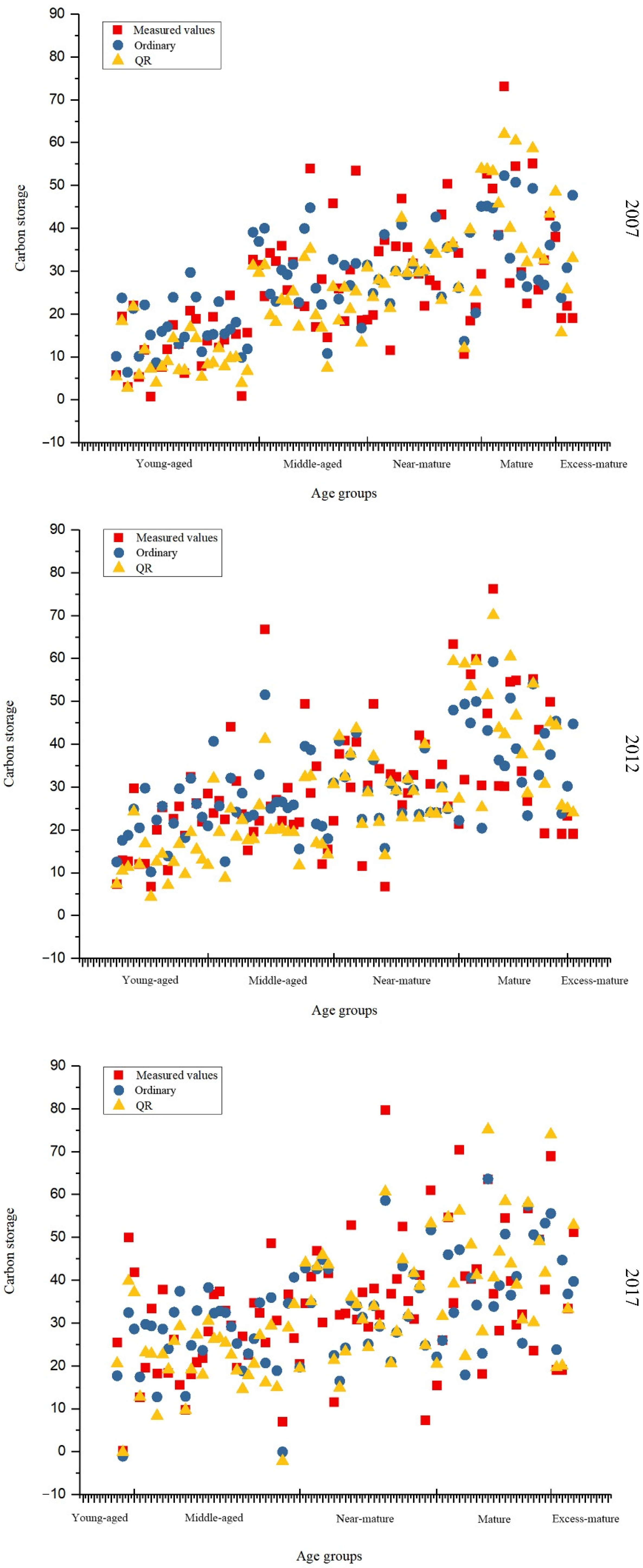
4.5. Model Prediction

To better compare the prediction accuracy of the two panel data models on Pinus kesiya var. langbianensis carbon storage, the results of the ordinary panel data model based on least squares, the quantile model, and the measured actual values were plotted as shown in Figure 4.

5. Discussion

This thesis is a good attempt to apply the ideas of panel data in economics for solving problems in forestry. Previous research on dynamic forest carbon storage involved complicated processing; it had to build up models for different periods, respectively, which was tedious and time-consuming. A panel data model can effectively solve this problem. Through the mixing of time series and cross-sectional data, panel data provides more informative data. The variability of variables is increased, the collinearity between variables is weakened, and the df and effectiveness are improved. Panel data can also better detect and measure effects that cannot be observed using purely cross-sectional data or time-series data.

In order to better understand the application of panel data in forestry, this paper used two models: an ordinary panel data model and a quantile-regression panel data model. For the ordinary regression model, all variables were significant (p < 0.01), and their coefficients were all positive, except for the constant term. Therefore, in the ten years from 2007 to 2017, the DBH, crown density, and altitude all had positive effects on Pinus kesiya var. langbianensis natural forest carbon storage. The elasticity coefficient of the DBH was the largest, at 2.1523, indicating that the average carbon sequestration increased by 2.15% when the average DBH increased by 1%. Crown density had the second most important influence, followed by altitude, which had the least effect.

In the quantile-regression results, average DBH coefficients significantly increased from 1.4635 to 2.6163, indicating a positive effect at both low- and high-quantiles and that it increased gradually from young-aged to over-mature forests. Crown density coefficients similarly changed from low- to high-quantiles, but the degree of change was relatively small. These results confirm the natural law that the amount of carbon sequestered in the forest increases as the DBH and crown density rise. Even if the DBH only increases slightly, forest carbon sequestration will change significantly, and it is especially true for mature and over-mature forests. Altitude, exerting similar effects as the first two variables, is statistically significant and has a positive regression coefficient. Although the variation remains within 0.008, it suggests that trees growing at higher elevations (cooler places) have a greater sequestration capacity. However, the changes were small, indicating that its influence on carbon storage of differently aged groups of Pinus kesiya var. langbianensis, was insignificant.

Through comparisons in Table 7, we found that coefficients estimated by the ordinary model were at average levels. For the altitude, its effect on estimated average carbon storage was small, but for the average DBH and crown density, large errors became apparent if their data differed among different age groups to large extents.

Secondly, residuals estimated by the ordinary panel data model were obvious, regardless of the survey year (2007, 2012 or 2017). The residuals increased gradually with natural forest carbon sequestration, and in terms of the age group, they were large in mature and over-mature forests. For the quantile-regression model, the overall residual distribution was more random, and there was no obvious heteroscedasticity. For young-aged and over-mature forests especially, the residual distribution was significantly more clustered compared to the ordinary panel data model. At the same time, compared with the ordinary model residuals, those of the quantile model were distributed in a smaller range, especially for young-aged and middle-aged forests. This provides further evidence for the unique advantage of quantile regression in fitting data with extreme values and outliers, and the effect of heteroscedasticity on the model is eliminated.

Table 8 showed that the quantile-regression model fit the data better at 0.1 quantiles and 0.9 quantiles with a lower AIC, MSE, MAE and higher R² than the ordinary regression model. There’s not much difference between the statistics of model fitting and testing, but this also shows that quantile panel data regression is more advantageous in estimating young-aged and over-mature forests. A young-aged forest is the stage of forest growth and development. An over-mature forest is a stage that has exceeded the mature stage and began to decline in growth and development, which can be cut. Accurate estimation of these two parts can provide better assistance to forestry management and harvest.

The results of the two models partially overlap with measured values (Figure 4). In terms of the age group, the quantile-regression results were closer to the measured values of young-aged, mature, and over-mature forests, while the ordinary regression results were relatively close to those of middle-aged forests, but for other age groups, the differences are generally large. It normally overestimates data for young-aged and middle-aged forests and underestimates data for near-mature up to over-mature forests. When considering that forests classified into different age groups change over time, the two model results were more different from measured values, especially for young-aged forests, and underestimation generally increased. Yet, compared with the ordinary model, the quantile-regression model produced results closer to reality, demonstrating that it can solve overestimation for young-aged forests and underestimation for over-mature forests.

Studies have shown that the quantile-regression model is better than the OLS model in the estimation of forest biomass and carbon storage, regardless of model fitting or sample testing [32], which is similar to the dynamic law discussed in this paper.

Therefore, Pinus kesiya var. langbianensis carbon sequestration at different time points can be predicted, and with the changing coverage of age groups considered, overall trends can be identified to facilitate dynamic predictions. As we found, average carbon sequestration of different age groups changes with time to some extent, with the greatest difference in the young-aged and the least in the over-mature forest. The highest carbon density in the first two surveys was in mature forests, while in 2017, it was for near-mature forests. This means mature and near-mature forests have the strongest carbon sequestration capacity, which is consistent with natural laws.

The meteorological data in this study was derived from “China Annual Surface Climatological Data Set station”. There are only 28 stations in the whole province of Yunnan. Altitude is not considered in the interpolation, so the interpolation results only represent the average change of the region, with little difference, whereas the forest of Pinus kesiya var. langbianensis is distributed in mountainous areas, and altitude is a significant-influence factor. Altitude can influence the distribution and growth of forests to a certain extent by affecting light, heat, runoff, and soil properties, thus affecting the carbon input of forest ecosystems. This also shows from the side that the temperature and precipitation have an impact on the carbon sequestration capacity of forests. Meanwhile, terrain characteristics were collected in this paper, but none of them were significant. According to the research results of this paper, the local variation of the terrain is not the main influencing factor, which is also related to the scale of data collection.

The model needs further improvement, possibly to set up meteorological data collection stations in the sample plots or transform the data collection scale, and for different forest species, the rule of changes in a longer period cannot be further discussed. In a follow-up study, we will require more data collection in the future and incorporate more environmental factors for improvement.

6. Conclusions

We built an ordinary model and a quantile-regression model using panel data from 243 sample plots of Pinus kesiya var. langbianensis in Yunnan provinces and used them in an age-group-based analysis. We obtained the following conclusions:

(1) Only data that indicated continuous and natural changes were considered. Sample plots where final felling had been conducted or where they were newly established were not considered. In linear regression modeling based on panel data, only the stand factors that were easily measured, such as the average DBH and crown density, were adopted to make the model simpler and easier to apply. Additional factors such as the altitude and terrain characteristics were also included to more fully cover environmental influences. Of these, only altitude showed a good linear correlation with average carbon sequestration of the natural forest sample plots. In summary, we selected the average DBH, crown density, and altitude. Altitude had relatively small effects on carbon sequestration, while the average DBH and crown density had more significant effects. Changes in carbon content with the DBH and crown density varied among different age groups and with time, while the effect of altitude was consistent among different age groups.

(2) From the 2007 cross-sectional data results, the overall relative error and absolute relative error of the quantile-regression model were lower than those of the ordinary regression model in both residual analysis and model prediction. In terms of the age group, the quantile-regression model was more accurate than the ordinary model for accurately predicting carbon storage in young-aged and mature forests and significantly lowered overestimation for young-aged forests and underestimation for over-mature forests.

(3) Because the structure of age groups changes over time, estimates of carbon sequestration by the models differed considerably from the actual measured values, and they often suffered underestimation, especially for some young-aged. Even though it was a common problem for both models, quantile model errors were smaller than for the ordinary model. This shows that in ordinary modeling, where sample plots are taken as a whole for evaluating effects, effects on different age groups are not determined. It also confirms that the fitting effect of the quantile model is better than that of the ordinary model. This model can also be used to predict values of different cross-sections and better grasp carbon sequestration changes with time.

Panel data models are usually used in the field of economics and have not yet been introduced into forestry research. We used this method for the first time in forestry research and showed that two panel-data-based methods could be used to model forest carbon sequestration because of its characteristic data with obvious trends. In this way, laws could be explored to better understand the trend of development. This paper is an approach to explore. Due to limited data access, explanations for more general laws of change over a longer period and for other species could not be discussed and will require more studies in the future.

References

1. Fang, J.; Guo, Z.; Hu, H.; Kato, T.; Muraoka, H.; Son, Y. Forest biomass carbon sinks in East Asia, with special reference to the relative contributions of forest expansion and forest growth. Glob. Chang. Biol. 2014, 20, 2019–2030. [Google Scholar] [CrossRef]
2. Harris, N.L.; Gibbs, D.A.; Baccini, A.; Birdsey, R.A.; de Bruin, S.; Farina, M.; Fatoyinbo, L.; Hansen, M.C.; Herold, M.; Houghton, R.A.; et al. Global maps of twenty-first century forest carbon fluxes. Nat. Clim. Chang. 2021, 11, 234–240. [Google Scholar] [CrossRef]
3. Soimakallio, S.; Kalliokoski, T.; Lehtonen, A.; Salminen, O. On the trade-offs and synergies between forest carbon sequestration and substitution. Mitig. Adapt. Strateg. Glob. Chang. 2021, 26, 1–17. [Google Scholar] [CrossRef]
4. Mader, S. Plant trees for the planet: The potential of forests for climate change mitigation and the major drivers of national forest area. Mitig. Adapt. Strateg. Glob. Chang. 2020, 25, 519–536. [Google Scholar] [CrossRef]
5. Falkowski, P.; Scholes, R.J.; Boyle, E.; Canadell, J.; Canfield, D.; Elser, J.; Gruber, N.; Hibbard, K.; Hogberg, P.; Linder, S.; et al. The global carbon cycle: A test of our knowledge of earth as a system. Science 2000, 290, 291–296. [Google Scholar] [CrossRef] [Green Version]
6. Granier, A.; Ceschia, E.; Damesin, C.; Dufrêne, E.; Epron, D.; Gross, P.; Lebaube, S.; Le Dantec, V.; Le Goff, N.; Lemoine, D.; et al. The carbon balance of a young Beech forest. Funct. Ecol. 2000, 14, 312–325. [Google Scholar] [CrossRef]
7. Law, B.E.; Thornton, P.E.; Irvine, J.; Anthoni, P.M.; Van Tuyl, S. Carbon storage and fluxes in ponderosa pine forests at different developmental stages. Glob. Chang. Biol. 2001, 7, 755–777. [Google Scholar] [CrossRef]
8. Hazlett, P.W.; Gordon, A.M.; Sibley, P.K.; Buttle, J.M. Stand carbon stocks and soil carbon and nitrogen storage for riparian and upland forests of boreal lakes in northeastern Ontario. For. Ecol. Manag. 2005, 219, 56–68. [Google Scholar] [CrossRef]
9. Neilson, E.T.; MacLean, D.A.; Meng, F.R.; Arp, P.A. Spatial distribution of carbon in natural and managed stands in an industrial forest in New Brunswick, Canada. For. Ecol. Manag. 2008, 253, 148–160. [Google Scholar] [CrossRef]
10. Gundersen, P.; Thybring, E.E.; Nord-Larsen, T.; Vesterdal, L.; Nadelhoffer, K.J.; Johannsen, V.K. Old-growth forest carbon sinks overestimated. Nature 2021, 591, 21–23. [Google Scholar] [CrossRef] [PubMed]
11. Siddiq, Z.; Hayyat, M.U.; Khan, A.U.; Mahmood, R.; Shahzad, L.; Ghaffar, R.; Cao, K.F. Models to estimate the above and below ground carbon stocks from a subtropical scrub forest of Pakistan. Glob. Ecol. Conserv. 2021, 27, e01539. [Google Scholar] [CrossRef]
12. Silva, H.F.; Ribeiro, S.C.; Botelho, S.A.; Liska, G.R.; Cirillo, M.A. Biomass and Carbon in a Seasonal Semideciduous Forest in Minas Gerais. Floresta E Ambiente 2018, 25, e20160508. [Google Scholar] [CrossRef]
13. Reiersen, G.; Dao, D.; Lütjens, B.; Klemmer, K.; Zhu, X.; Zhang, C. Tackling the Overestimation of Forest Carbon with Deep Learning and Aerial Imagery. arXiv 2021, arXiv:2107.11320. [Google Scholar]
14. Nie, X.; Guo, W.; Huang, B.; Zhuo, M.; Li, D.; Li, Z.; Yuan, Z. Effects of soil properties, topography and landform on the understory biomass of a pine forest in a subtropical hilly region. Catena 2019, 176, 104–111. [Google Scholar] [CrossRef]
15. Liu, C.; Zhang, L.; Li, F.; Jin, X. Spatial modeling of the carbon stock of forest trees in Heilongjiang Province, China. J. For. Res. 2014, 25, 269–280. [Google Scholar] [CrossRef]
16. Smeglin, Y.H.; Davis, K.J.; Shi, Y.; Eissenstat, D.M.; Kaye, J.P.; Kaye, M.W. Observing and Simulating Spatial Variations of Forest Carbon Stocks in Complex Terrain. J. Geophys. Res. Biogeosci. 2020, 125, e2019JG005160. [Google Scholar] [CrossRef]
17. Sun, W.; Zhu, Y.; Huang, S.; Guo, C. Mapping the mean annual precipitation of China using local interpolation techniques. Theor. Appl. Climatol. 2015, 119, 171–180. [Google Scholar] [CrossRef]
18. Sun, Y.S.; Wang, W.F.; Li, G.C. Spatial distribution of forest carbon storage in Maoershan region, Northeast China based on geographically weighted regression kriging model. J. Appl. Ecol. 2019, 30, 1642–1650. (In Chinese) [Google Scholar]
19. Luyssaert, S.; Schulze, E.D.; Börner, A.; Knohl, A.; Hessenmöller, D.; Law, B.E.; Ciais, P.; Grace, J. Old-growth forests as global carbon sinks. Nature 2008, 455, 213–215. [Google Scholar] [CrossRef]
20. Litvak, M.; Miller, S.; Wofsy, S.C.; Goulden, M. Effect of stand age on whole ecosystem CO2, exchange in the Canadian boreal forest. J. Geophys. Res. Atmos. 2003, 108, 171–181. [Google Scholar] [CrossRef] [Green Version]
21. Zaehle, S.; Sitch, S.; Prentice, I.C.; Liski, J.; Cramer, W.; Erhard, M.; Hickler, T.; Smith, B. The importance of age-related decline in forest NPP for modeling regional carbon balances. Ecol. Appl. 2006, 16, 1555–1574. [Google Scholar] [CrossRef]
22. Williams, M.; Schwarz, P.A.; Law, B.E.; Irvine, J.; Kurpius, M.R. An improved analysis of forest carbon dynamics using data assimilation. Glob. Chang. Biol. 2010, 11, 89–105. [Google Scholar] [CrossRef]
23. Zhao, M.; Yue, T.; Zhao, N.; Sun, X.; Zhang, X. Combining LPJ-GUESS and HASM to simulate the spatial distribution of forest vegetation carbon stock in China. J. Geogr. Sci. 2014, 24, 249–268. [Google Scholar] [CrossRef]
24. Hallock, K.F.; Koenker, R.W. Quantile Regression. J. Econ. Perspect. 2001, 15, 143–156. [Google Scholar]
25. Jin, B.; Wu, Y.; Rao, C.R.; Hou, L. Estimation and model selection in general spatial dynamic panel data models. Proc. Natl. Acad. Sci. USA 2020, 117, e201917411. [Google Scholar] [CrossRef]
26. Bera, A.K.; Doğan, O.; Taşpınar, S.; Leiluo, Y. Robust LM tests for spatial dynamic panel data models. Reg. Sci. Urban Econ. 2019, 76, 47–66. [Google Scholar] [CrossRef]
27. Wooldridge, J.M. Econometric Analysis of Cross-Section and Panel Data; MIT Press: Cambridge, MA, USA, 2001; Volume 1, pp. 206–209. [Google Scholar]
28. Lu, X.; Su, L. Determining individual or time effects in panel data models. J. Econom. 2020, 215, 60–83. [Google Scholar] [CrossRef]
29. Jari, K.; Olli, T. Testing the Forest Rotation Model: Evidence from Panel Data. For. Sci. 1999, 45, 539–551. [Google Scholar]
30. Ou, G.L.; Xu, H. Construction of an Environment-Sensitive Biomass Model for Natural Pinus Simaosi Forest; Science Press: Beijing, China, 2015. (In Chinese) [Google Scholar]
31. Zang, H.; Liu, S.; Huang, J.C.; Zhang, Z.D.; Ouyang, X.Z.; Ning, J.K. Effects of Competition, Climate Factors and Their Interactions on Diameter Growth for Chinese Fir Plantations. Sci. Silvae Sin. 2021, 57, 12. (In Chinese) [Google Scholar]
32. Yuan, S.K.; Xu, H.; Li, C.; Lv, Y.L.; Wei, A.C.; Xiong, H.X.; Ou, G.L. Remote sensing estimation on biomass of Pinus densata forests based on quantile regression model. For. Inventory Plan. 2018, 43, 8–13; discussion 14–31. (In Chinese) [Google Scholar]
Figure 1. Sample plot distribution.
Forests 13 00012 g001
Figure 2. Model selection.
Forests 13 00012 g002
Figure 3. Residual plots of the ordinary model and the quantile model.
Forests 13 00012 g003
Figure 4. The results of the ordinary panel data model based on least squares, the quantile model, and the measured actual values.
Forests 13 00012 g004