Modeling the Dominant Height of Larix principis-rupprechtii in Northern China—A Study for Guandi Mountain, Shanxi Province

Abstract

An accurate estimate of the site index is essential for informing decision-making in forestry. In this study, we developed site index (SI) models using stem analysis data to estimate the site index and the dominant height growth for Larix gmelinii var. principis-rupprechtii in northern China. The data included 5122 height–age pairs from 75 dominant trees in 29 temporary sample plots (TSPs). Nine commonly used growth functions were parameterized using the modeling method, which accounts for heterogeneous variance and autocorrelation in the time-series data and introduces sample plot-level random effects in the model. The results show that the Duplat and Tran-Ha I model with random effects described the largest proportion of the dominant height variation. This model accurately evaluated the site quality and predicted the dominant tree height growth in natural Larix forests in the Guandi Mountain region. As an important supplement in improving methods for site quality evaluation, the model may serve as a fundamental tool in the scientific management of larch forests. The research results can inform an accurate evaluation of the site quality and predict the growth of the dominant height in a larch forest in the Guandi Mountain forest area as well as provide a theoretical basis for forest site quality evaluation at similar sites.

1. Introduction

Larix gmelinii var. principis-rupprechtii (larch) forests occupy approximately 65% of the forested land in northern China. These larch forests are mostly managed for timber production, ecosystem or watershed protection, and as habitats for wild animals. Larch forests in this region are usually characterized by a large amount of biomass and high primary productivity. Many studies have demonstrated that larch forests play critical roles in regional carbon storage and carbon cycling [1,2,3,4,5].

For a given tree species, a site index (SI) model (or top height growth models) is the most commonly used tool to estimate the potential site productivity, which is defined as the expected average height of dominant trees at the selected reference age [6,7]. Dominant height growth models, also known as SI models, are commonly used to estimate the potential productivity of forest stands. Predicting the maximum possible (potential) height growth is one of the most important components of forest growth and yield modeling [8,9,10].

To estimate the SI more accurately, it is necessary to adjust the appropriate SI model according to the local site conditions. In forestry practice in northern China, a site class is still determined using height growth curves. The production of a tree growth curve is complex and will produce different errors with different drafts [11]. Dominant heigh models have only been developed for some species (Pinus tabuliformis [12] and Cunninghamia lanceolata [13]) in this region. Based on the importance of larch in the ecosystem, there is a lack of relevant dominant height models in Shanxi, Guangdi Mountain. Therefore, it is necessary to develop a dominant height model for larch.

When building an SI model, both dynamic (base age unchanged) and static equations (depending on base age) have been used [11]. Many growth model equations have been used to establish the dominant height model. Mitscherlich, Gompertz, modified Gaussian, log-logistic, and variations of these models have been the most used in dominant height modeling [14,15,16,17]. Data from temporary sample plots (TSP), permanent sample plots (PSP), and stem analyses (SA) are often used to develop dominant height growth models and simulate site index curves. PSPs are considered the best source for building dominant height growth models [18,19,20]. However, PSP data can be attributed to multiple measurements from the same subjects, comprising of both plots and trees, which requires more resources compared with SA data. Compared with SA data, TSP data are more difficult to investigate resulting in higher economical and temporal investments. This is because they can be used to deduce the past height growth from growth-ring observations from the dissected trees being sampled. SA is the fastest approach for obtaining extensive growth information without the need to obtain long-term records [14,20]. However, SA data are repeated measurements of the same tree, and the data obtained will have a time-series correlation and be structured hierarchically. Thus, the measurements or data are hierarchically structured and most likely spatially correlated to each other [21,22]. In this case, the assumption of independent errors is violated when the ordinary least squares (OLS) is applied to estimate the model parameters in the forest mortality models. This would result in biased estimations of the variances of the parameter estimates and thus invalidate the hypothesis tests of parameter estimates [23]. Therefore, it is necessary to use the nonlinear mixed-effects (NLME) method to solve the above problems. In recent years, this approach has been increasingly used to develop various forest models, including forest growth models [1,2,3,24,25,26], to efficiently analyze hierarchically structured data, and increase prediction accuracy [1,2,3,23]. There are some research methods that can hierarchically structure data, and there are only a few studies on the correlation of time-series data of dominant height [1,2,3,23,24,25,26].

To develop a dominant height growth model for Larix gmelinii var. principis-rupprechtii in northern China and to solve the problem of hierarchically structured data and correlated observations, this study aims to (1) develop dominant height models for the larch forests by applying mixed-effects modeling; (2) predict the tree height growth, site index, and the maximum productivity level. The model presented will be useful for site quality evaluation in the northern Chinese natural larch forest in the Guandi Mountain forest region and the adjacent forest areas. These site index curves constitute the first step toward producing new yield tables.

2. Materials and Methods

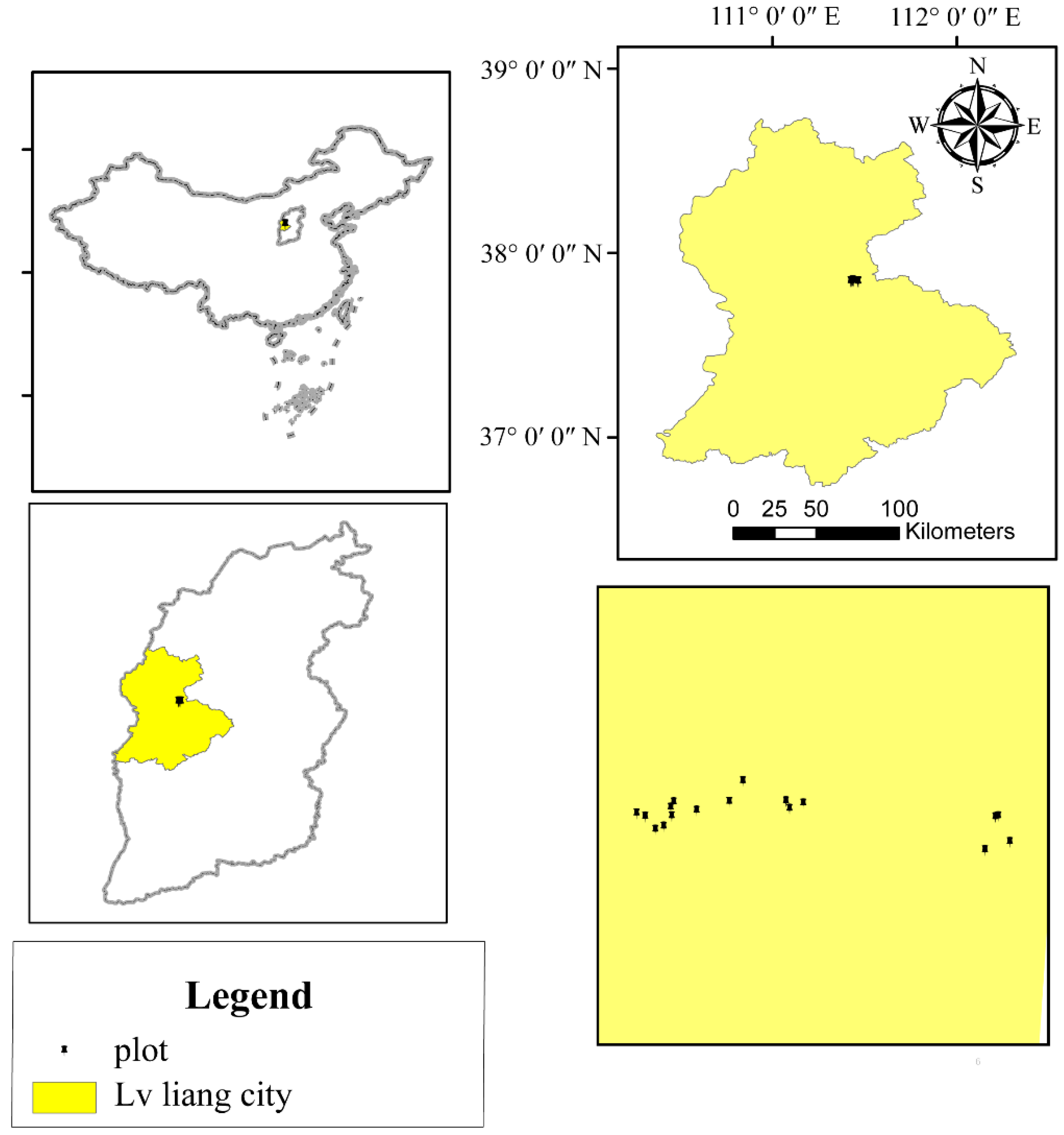
2.1. Study Areas

The Guandi Mountain National Forest Park is located in the middle of Shanxi Province, which spans the Jiaocheng and Fangshan counties. The geographical coordinates are 111°22′–111°33′ E, 37°45′–37°55′ N, encompassing an area of 76,135 hectares, with a forest cover rate of more than 75%. The landform is a large, undulating mountain with strong denudation. The main rock types are granite, gneiss, diabase, quartzite, and amphibolite. The study area has a temperate continental climate [27]. The annual average temperature is approximately 4.3 °C, the average temperature during the hottest month (July) is 17.5 °C, and the average temperature during the coldest month (January) is −10.2 °C. There is a frost-free period of approximately 100–125 days and the average annual precipitation is 822.6 mm.

2.2. Sampling and Measurement

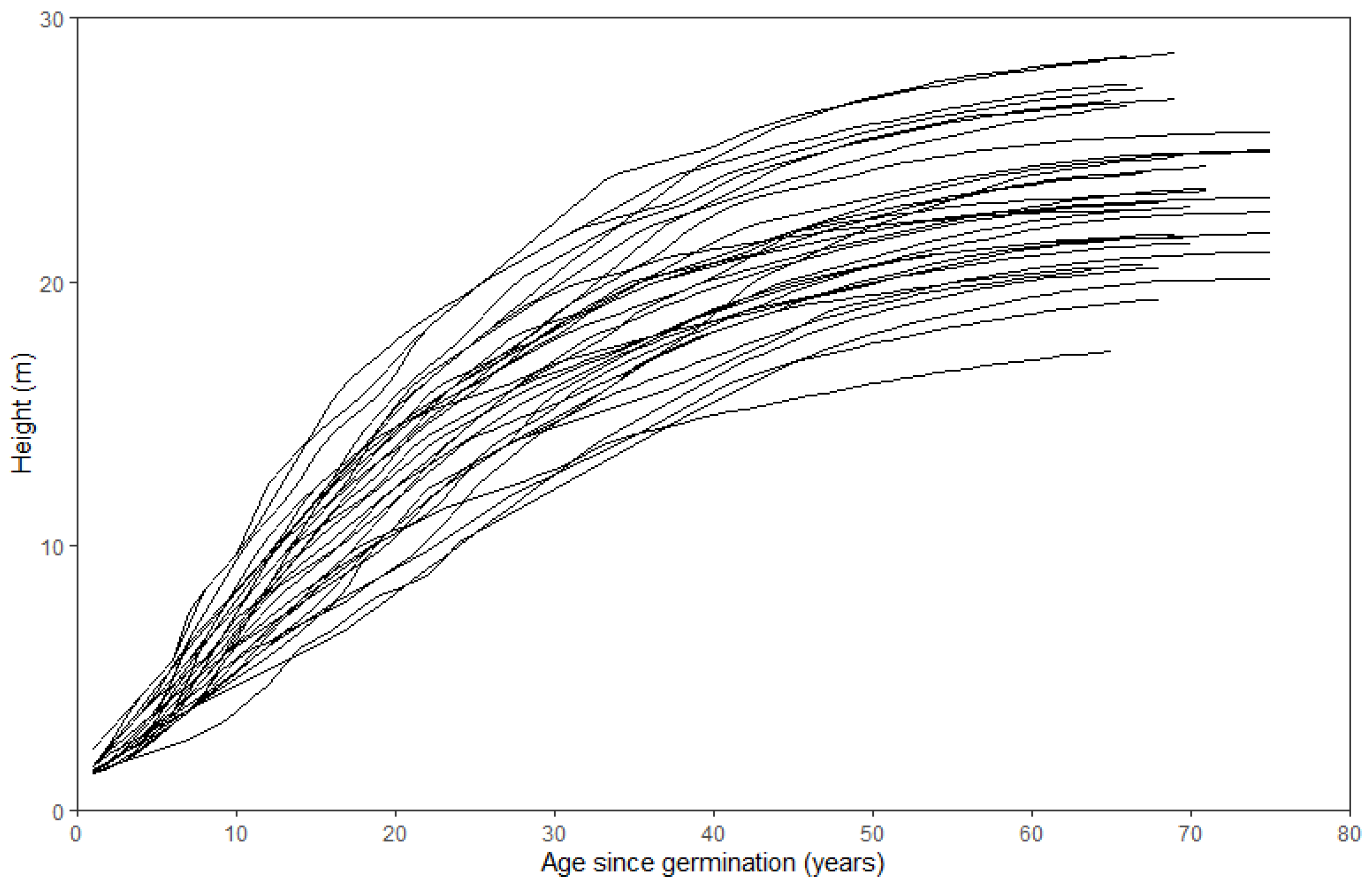
Data collection for this study was completed through a combination of fieldwork and indoor experiments. The stands that were sampled include the most diversified site conditions where larch is found on Guandi Mountain to represent the largest possible range of site indices. In September 2015, through understanding the site types of larch on Guandi Mountain, the eight most common site types were selected, and then 29 temporary sample plots (TSPs) were set up (

Table 1. Distribution of dominant larch trees in different site types.

Site Type	Number of Dominant Trees	Stand Age	Number of Plots	Slope (°)
Sunny slope, thick soil, and middle-elevation area	7	57–75	2	6
Sunny slope with medium or thick soil in the middle-elevation area	9	67–75	4	7
Shady slope, thick soil, and middle-elevation area	8	59–73	3	9
Shady slope with medium or thick soil in the middle-elevation area	9	55–75	4	8
Sunny slope, thick soil, and high-elevation area	14	64–75	5	6
Sunny slope with medium or thick soil in the high-elevation area	11	68–75	4	8
Shady slope, thick soil, and middle- and high-elevation areas	9	57–75	4	7
Shady slope with medium or thick soil in the high-elevation area	8	62–72	3	8

). These sample plots cover a large area of forest, with sufficient changes in stand structure, stand density, tree size, stand age, site productivity, terrain, and environmental settings (including the soil and slope). Each sample plot was 20 m × 20 m (Figure 1). All the standing and living trees with a diameter at breast height (DBH) ≥ 5 cm were measured for DBH, total height (H), height to live crown base, and the four crown radii. Four dominant or codominant trees representing the four largest trees in a 400 m² TSP or the 100 largest trees ha^{− 1} [1] were identified and measured in each plot. For each TSP, dominant tree DBH (DD) and dominant tree H (DH) were obtained from the arithmetic means of these attributes [1,2,3]. A total of 75 trees of dominant height were identified for felling in the 29 pure larch stands aged 40–75 years (Figure 2).

2.3. Stem Analysis

Before felling the trees being sampled, the position in the north-south direction and the diameter at breast height (DBH) were marked on the trunk. The DBH and the tree height were measured after the larch had been cut. Discs were taken from each section at 0 m, 0.3 m, 0.8 m, 1.3 m, and the position above 1.3 m. Discs were cut at 2 m intervals above DBH. The sampling positions were at 3.3 m, 5.3 m, 7.3 m, etc. When the remaining larch stem tip was less than 2 m, the entire stem was sampled. The north-south direction, sample plot number, stem number, and disc height were recorded on the non-working surface of the disc. The disc thickness was 4 cm (2 cm above and 2 cm below the line). The cut discs and the remaining larch stem tip were taken back to the laboratory and placed in a cool and ventilated place for drying.

After they had been dried, the working surfaces of the discs were polished, scanned, and then archived. Fine sandpaper with an average particle diameter of 140 mm was used to grind the discs. Annual ring analytical data were obtained by using a Windendro ring analysis instrument (Canada, 2015) to scan the polished discs (Canada, 2015) [27]. Xlstem software was used to analyze tree ring data and obtain the analytic tree data [27,28]. The Carmean method [28] was used to correct the tree height bias. The tree height growth process was analyzed by drawing the tree height–age curve for individual trees. As larch is a strong plant and a shade-intolerant tree species, it will not build up shade tolerance and cannot survive for long periods of suppression. Thus, by drawing the tree height–age curve and analyzing the relationship between tree height growth and age, 75 dominant trees’ stem analysis data in the natural forest could be obtained. The SA dataset comprised 5122 height–age pairs encompassing heights from 1.39 to 28.81 m and ages ranging from 1 to 75 years (Table 1).

The 75 trees were randomly split into two groups: A total of 61 trees were used for model fitting and 14 trees were used for model validation.

2.4. Base Models

We used eight growth functions (

Table 2. Various forms of the growth functions (as base functions) tested for the dominant height growth models of larch. The parameter describing the productivity level is always represented by “b_i” (asymptotic parameter), the shape parameters are represented by “a”, “c”, and “d”, and DH is dominant height.

Name	Formulation	Designation	Source
Mitscherlich	$DH=b_i\ast [1-e^{\frac{(a-age)}{c}}]$	(1)	[29]
Gompertz	$DH=b_i\ast [-e^{\frac{(a-age)}{c}}]$	(2)
Modified Gaussian	$DH=b_i\ast [1-e^{-\frac{(age-a)}{c^2}}]$	(3)
Log-logistic	$DH=\frac{b_i}{1+{(\frac{age}{a})}^{-c}}$	(4)
Chapman–Richards anamorphic	$DH=b_i\ast e^{{(-a\ast age)}^c}$	(5)	[30]
Bailey and Clutter	$DH=e^{(b_i+a\ast ({(\frac{1}{age})}^c))}$	(6)	[31]
Duplat and Tran-Ha I	$DH=(a\ast age+b_i)\ast (1-e^{(-({(\frac{age}{c})}^d))}$	(7)	[32]
Duplat and Tran-Ha II	$DH=(a\ast Ln(age)+b_i)\ast (1-e^{(-({(\frac{age}{c})}^d))})$	(8)

Notes: $DH$ is the dominant tree height observed, and age indicates the age corresponding to the dominant tree height. b_i, a, c, and d are the parameters to be estimated.

) that are commonly used for dominant height growth modeling [14,29,30,31,32] to fit the height data.

Researchers have used a range of mathematical functions to describe the stand growth. We also selected a commonly used form of the ADA model. Model 9 [20] is a growth model that has been frequently tested in many studies on SI modeling (

Table 3. The dynamic generalized algebraic difference approach (GADA) formulations with base equations used to model the dominant height growth.

Base Model Forms	Parameters Related to Site and Solution for Theoretical Variable X	Dynamic GADA Formulation	Designation	Source
$DH=\frac{ag{e}^2}{a_1+a_{2}age+a_{3}ag{e}^2}$	$a_2=X$ $X_0=\frac{ag{e}_0}{D{H}_0}-\frac{b_1}{ag{e}_0}-b_{2}ag{e}_0$	$D{H}_1=\frac{ag{e}_1{}^2}{a+X_{0}ag{e}_1+bag{e}_1{}^2}$	(9)	[20]

Notes: a₁, a₂, and a₃ are parameters in the base models; b₁ and b₂ are parameters in the dynamic models; DH₀ and DH₁ are heights (in m) at age₀ and age₁ (in years), respectively; X₀ is the solution of X for the initial height and age.

) [20,33,34].

We estimated the model parameters and selected the best-performing model for further analysis using the following four statistical criteria:

$$R^2=1-{\displaystyle \sum _{i=1}^n{(D{H}_i-{\widehat{DH}}_i)}^2}/{\displaystyle \sum _{i=1}^n{(D{H}_i-{\overline{DH}}_i)}^2}$$

(10)

$$MD=\frac{1}{n}{\displaystyle \sum _{i=1}^n(D{H}_i-{\widehat{DH}}_i)}$$

(11)

$$RMSE=\sqrt{\frac{1}{n}{\displaystyle \sum _{i=1}^n{(D{H}_i-{\widehat{DH}}_i)}^2}}$$

(12)

$$TRE={\displaystyle \sum _{i=1}^n\left|D{H}_i-{\widehat{DH}}_i\right|}/{\displaystyle \sum _{i=1}^n{\widehat{DH}}_i}$$

(13)

where $D{H}_i$ is the observed dominant height, $\widehat{D{H}_i}$ is the estimated dominant height, $\overline{D{H}_i}$ is the average dominant height, and n is the number of sample heights.

The graphical appearance and numerical statistics were then examined for the fitted models, where $R^2$ is the coefficient of determination, MD is the mean residual error, $RMSE$ is the root mean square error, and $TRE$ is the total relative error.

2.5. Nonlinear Mixed-Effects (NLME) DH Model

By introducing plot-level random effects, the best-fitting model identified from this procedure was used to formulate the NLME models. The NLME model, which comprises all possible combinations of the fixed-effect parameters with random effects at the plot level, was fitted to the data. We chose the model with the smallest AIC and the largest log-likelihood (LL) for further analysis. To avoid problems derived from over-parameterization, we performed a likelihood-ratio test (LRT) [35].

The residuals of the NLME DH model with random effects at the plot level were analyzed for potential autocorrelations among observations on the same subjects.

To account for the within-sample plot variance–covariance matrix ($R_i$) of the error term ($e_{ij}$), the following expression was used:

$$R_i={\sigma }^2{G}_i^{0.5}{\Gamma }_i{G}_i^{0.5}$$

(14)

where $R_i$ is the variance–covariance matrix of the error within sample plot i, ${\sigma }^2$ is a scaling factor of the error dispersion, which is equal to the residual variance of the estimated model, $G_i$ is the diagonal matrix of the within-plot heteroscedasticity variances, and ${\Gamma }_i$ is the matrix showing the within-plot autocorrelation structure of the errors. Therefore, ${\Gamma }_i$ is assumed to be an identity matrix.

The heteroscedasticity problem in our analysis was eliminated using a variance-stabilizing function. We evaluated the three variance functions using stand age as a predictor variable in the functions (Equations (15)–(17)) and identified the one that performed the most effectively. We selected the optimal variance-stabilizing function by evaluating the AIC and −2LL values.

$$Var({\xi }_{ij})={\sigma }^2\exp (2\gamma ag{e}_{ij})$$

(15)

$$Var({\xi }_{ij})={\sigma }^{2}ag{e}_{{}_{ij}}^{2\gamma }$$

(16)

$$Var({\xi }_{ij})={\sigma }^2{({\gamma }_1+ag{e}_{{}_{ij}}^{2{\gamma }_2})}^2$$

(17)

where age_ij indicates the age of the jth tree in the ith sample plot and $\gamma ,{\gamma }_1,{\gamma }_2$ represents the parameter to be estimated. The variance function was evaluated using AIC and log-likelihood [35,36]. All the NLME DH models were estimated using the maximum-likelihood method implemented in the NLME function in R 3.5.2 [17,21].

For the time-series autocorrelation problem for data, most studies have suggested that AR (1) can be eliminated [11,37]. We used the commonly used error effect variance first-order autocorrelation error structure (AR (1)) to eliminate this to ensure that model autocorrelation was reduced.

In this study, we also compared the improvement of the model only using the weight function, or AR (1), and using both simultaneously.

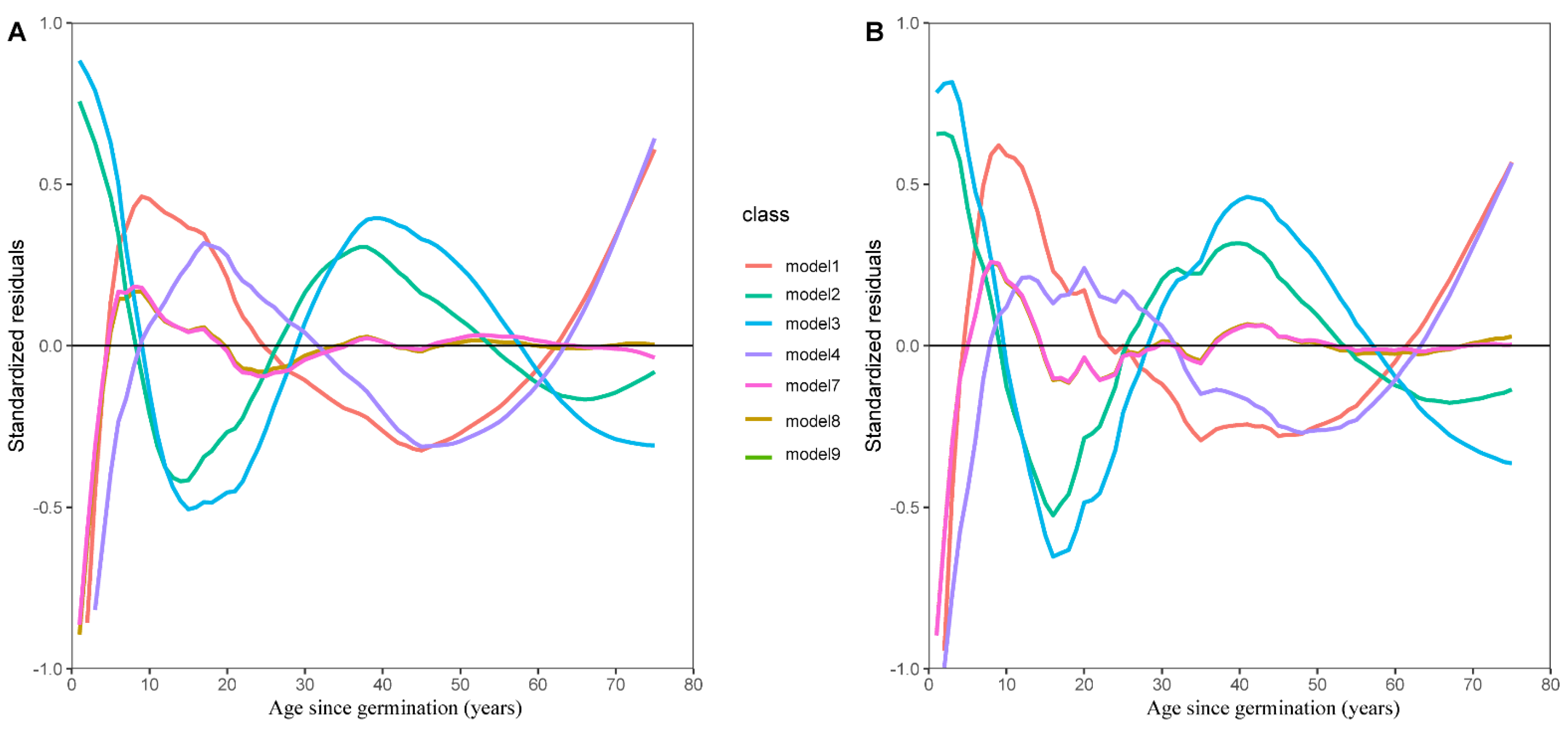
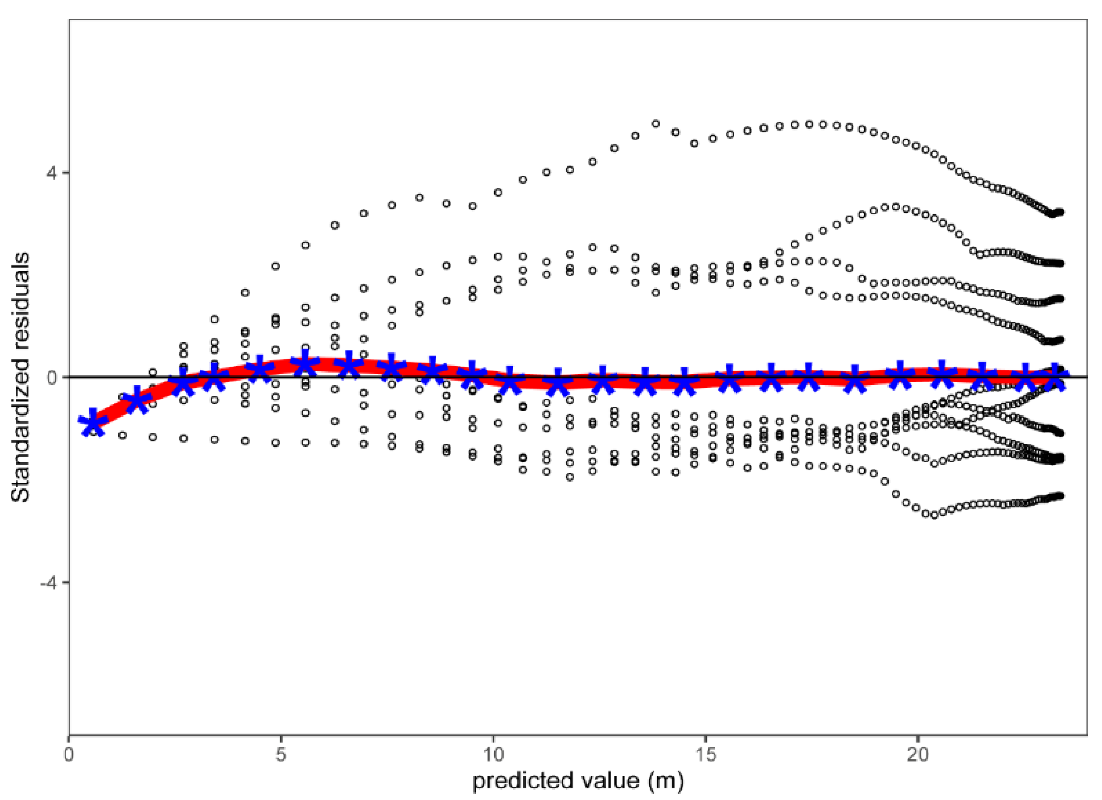
2.6. Model Evaluation

The statistics MD, TRE, R², and RMSE were calculated using Equations (10)–(13), which were applied to assess the prediction performance of the NLME DH model developed using the fitting and validation datasets. We estimated the models using the nlme package in R 3.6.3 [38].

3. Results

Following the original objective, we initially fitted nine different models (Table 2) to the SA data.

Table 4. Parameter estimation of nine candidate DH models (standard deviation) using modeling data.

Model	a	b	c	d
1	0.6846 (0.1551 ***)	26.1782 (0.2053 ***)	28.1981 (0.5923 ***)
2	13.3189 (0.1334 ***)	23.6106 (0.1093 ***)	14.3975 (0.2295 ***)
3	−10.2367 (0.3447 ***)	23.0135 (0.0927 ***)	−34.3262 (0.4830 ***)
4	23.7925 (0.6569 ***)	29.5419 (0.4642 ***)	1.3459 (0.0293 ***)
5	-	-	-
6	−6.9349 (0.2548 **)	3.7427 (0.0374 ***)	0.5956 (0.0229 ***)
7	55.2780 (17.0909 *)	−0.2938 (0.1438 ***)	63.8875 (22.9816 ***)	1.0400 (0.0332 ***)
8	259.4453 (236.4819)	−48.9553 (47.9220)	104.5320 (71.9311)	1.2811 (0.01528) ***
9	−1.6187 (0.0494 ***)	0.0234 (0.0003 ***)

Notes: values in parentheses are standard errors; “***”: p < 0.0001, “**”: p < 0.001,”*”: p < 0.05.

shows the parameter estimation for the nine candidate models. The fit statistics for the models and their validation statistics are summarized in

Table 5. Statistics of the converged base models for the model fitting and validation datasets (MD (mean prediction error), RMSE (root mean square error), TRE (total relative error), and R² (coefficient of determination)).

Model	Model Fitting Data				Model Validation Data
	MD	RMSE	TRE	R2	MD	RMSE	TRE
1	0.0001	2.4587	1.9925	0.8790	−0.0733	1.6564	0.8276
2	−0.0161	2.4482	1.9753	0.8800	−0.0896	1.6418	0.8130
3	−0.0179	2.4573	1.9903	0.8791	−0.0918	1.6625	0.8337
4	0.0416	2.4570	1.9898	0.8791	−0.0328	1.6460	0.8172
5	-	-	-	-	-	-	-
6	0.0626	2.4905	2.0456	0.8758	−0.0101	1.6982	0.8703
7	0.0131	2.4386	1.9595	0.8809	−0.0595	1.6262	0.7975
8	0.0158	2.4391	1.9603	0.8809	−0.0576	1.6260	0.7973
9	−0.0467	2.6324	2.2908	0.8613	−0.0598	1.9340	1.1490

.

The Chapman–Richards model did not converge. All the parameters were significant (p < 0.05), except for a, b, and c of Model 8. The other seven models showed better fit statistics, with small differences between them. Models 1–4 and 7–8 had better fit statistics and were comparable to each other (identical R², RMSE, and TRE values for both the fitting and validation data). The residuals for Models 1–4 and 7–9 are shown in Figure 3 to illustrate the residual variation of the mean residuals for the same age. When the forest was young (0–10 years old per tree), the fitting effect of the model was poor. In the other age groups (where every tree was older than 10 years old), Model 7 showed promising fit statistics (Figure 3), and these changes showed identical trends for the model fitting and the validation data. Graphical analyses of the error height are used to better explain the poorer fitting performance for the other candidate models (Figure 3). The Mitscherlich (1) and log-logistic (4) models were found to give a slight underestimation for tree height growth after age 60. The Gompertz (2) and modified Gaussian (3) models showed opposite results, and these models (1,2,3,4,9) inadequately expressed height growth for ages between 10 and 60. The Duplat and Tran-Ha I, II (7, 8) models provided an adequate fit to the data and were characterized by robust performance over the entire age range and site productivity levels (Figure 3).

We formulated dominant height growth models using Models 7 and 8 by incorporating random effects, which account for the sample plot-level variation.

Among the 15 parameter combinations that were evaluated, only adding bi provided the best fit (largest R² and smallest RMSE and TRE). By comparing the residual diagram with the model index (

Table 6. Parameter estimates, fit statistics, and standard errors of the model fitted statistics for the Duplat and Tran-Ha I and II parameterized models with random effects included (Equations (7) and (8)).

Model	Parameter Estimates				Random Effects	Fit Statistics
	a	b	c	d	${\mathit{\mu }}_{\mathit{i}1}$	R2	RMSE	TRE	LL
Model 7	22.1398	0.0348	23.4600	1.1566	1.5682	0.9060	2.1667	1.5403	−8963.653
Model 8	17.7929	1.6331	23.4646	1.0941	1.5785	0.9060	2.1669	1.5406	−8964.046

Notes: LL expresses the log-likelihood.

, Figure 3), we chose the nonlinear mixed-effects (NLME) Model 7 as the final dominant height growth model because its form is simpler than that of the other models. Among the three variance functions being tested (Equations (15)–(17)) and considering the time-series correlation, the power function (Equation (16)) + AR (1) accounted for variance heteroscedasticity and time-series correlations most effectively (

Table 7. Fit statistics of three variance functions (exponential function, power function, and constant plus power function) applied to the NLME DH model (LL, log-likelihood).

Variance Functions	NLME Model 7
	AIC	LL
Equation (15)	17766.92	−8876.46
Equation (16)	17500.2	−8743.10
Equation (17)	17502.19	−8743.097
Equation (15) + AR(1)	17705.89	−8844.944
Equation (16) + AR(1)	17466.55	−8725.273
Equation (17) + AR(1)	17468.55	−8725.273
AR(1)	17873.81	−8929.906

).

The final NLME DH model is given by:

$$DH=(a\ast age+b_i+{\mu }_i)\ast (1-e^{(-({(\frac{age}{c})}^d))})+{\zeta }_i$$

(18)

where DH is the dominant height (m); age is counted as germination; a, c, and d are the shape parameters; b_i is an asymptotic parameter or productivity level parameter; ${\mu }_i$ are the plot-level random-effect parameters, and ${\zeta }_i$ is the model residual vector.

A simple inversion of Equation (18) makes it possible to estimate b_i (the maximum productivity level) using any DH–age pair as follows:

$$b_i=\frac{DH}{(1-e^{(-({(\frac{age}{c})}^d))})}-a\ast age-{\mu }_i+{\zeta }_i$$

(19)

It is possible to estimate the past and future dominant height of a stand when at least one height–age pair is known. The estimation is performed using this pair to calculate b_i using Equation (18) and using the value obtained in Equation (20):

$$DH=(a\ast (age-ag{e}_0)+\frac{D{H}_0}{(1-e^{(-({(\frac{ag{e}_0}{c})}^d))})})\ast (1-e^{(-({(\frac{age}{c})}^d))})+{\zeta }_i$$

(20)

where the DH–age is the predicted height–age pairs and DH₀–age₀ is the observed value height–age pairs.

The residuals for Model 7 are shown in Figure 4 to illustrate the residual variation in the observed site indices. Analysis of residuals on the dominant height indicated that these were always equally distributed around zero, and there was no significant deviation greater than 5 m in the range of height, age, or productivity level. However, there was some deviation when the site index was less than 5 m (Figure 4).

The site index was estimated using Equation (20) from any height–age pair or to model the dominant height growth curve for a given SI.

We tested the model NLME7 fitted to the combined data against the independent dataset derived from the stem analysis of individual dominant trees (SA validation data). The prediction statistics for all the trees (RMSE = 1.6296, TRE = 0.8026, N = 14) indicated a good model fit for this dataset. The NLME7 model did not show a significant deviation for any age stand in the SA validation dataset (Figure 5).

Figure 6 shows the dominant height growth for different site indices. According to the fitting data, the model validity domain encompassed site indices between 14 and 26 m at 45 years of age.

4. Discussion

Many mathematical functions have been applied in the development of SI curves [8]. Choosing the best form to analyze the height–age relationship of trees in a specific area is of considerable importance for forest growth and harvesting. We evaluated nine base functions from different forms proposed in previous SI modeling studies [14,20,29,33,34,39]. Model 7 had the best fitting effect and thus was selected, and the random effect was introduced at the sample plot level. Therefore, our mixed-effects DH model (Equation (18)) was based on one predictor variable (age) and one random component to describe the sample plot-level random variation in DH.

The model selected had the characteristics required for an effective site index model for use in this study. The quality of the dataset is key to the success of fitting a growth model because this should include all the possible growth conditions of the forests, such as the age group and site productivity levels. In our study, this was achieved by analyzing SA data from mature larch forests. The sampling undertaken has been shown to fully represent the site characteristics of tree species distribution in this region. This means that our dataset covers a wider range of fertility levels from 14 to 26 m in height at age 45 than that represented in the yield tables of Zhang et al. (2016) for Guandi Mountain [27].

By selecting a model with a good fitting effect, Model 7 (Duplat and Tran-Ha I) showed the best performance. Similar results have been reported in other studies [10,40]. When the random effect was introduced at the plot level, the accuracy of the model improved considerably. When the validation dataset was used to test Model 7, the predicted residual error of larch at any dominant height was small (Figure 5). Therefore, the introduction of random effects can improve the accuracy of the model and explain the influence of different site conditions to a certain extent on the dominant height [2]. This may be because trees represent and reflect the characteristics of different sites. The age structure and the site productivity levels of the dominant tree species were found to be different in different sample plots. Because the random effects were added as b_i, the differences were explained as the effects of productivity in the different sample plots. We evaluated the three variance functions using stand age as the predictor variable to eliminate heteroscedasticity and the first-order autocorrelation error structure (AR (1)) to eliminate variance errors to ensure that the model autocorrelation was reduced. The use of these two functions provides a solution for later processing of the same class data.

Duplat and Tran-Ha I (Model 7) provided the best fitting performance for our dataset (Table 5). This may be because this model lacks horizontal asymptotes, whereas they are present in other models [14]. For stands with an average age of more than 200 years, there is no upper limit on the growth trajectory of the tree height [19,40]. This maximum tree height was not recorded in our dataset, and the model formula characterized by inclined asymptotes seems to be more appropriate.

Because of an unknown change in dominance during stand growth, the development of a height growth curve using SA data may lead to bias [17,41]. If a young forest has a dominant tree and its trunk is straight, it will always be the dominant tree during stand growth and development. When two identical dominant trees grow together in a young forest, the two trees interact to a certain extent; thus, one tree loses its dominant position. As larch is a strong tree species, it may die or not grow when it is restrained [42]. Moreover, no dead tree stumps were found in the study sample plot. Therefore, this ensures that the collected data are in a long-term dominant state. SA data acquired from straight trees and dominant trees with poor juvenile trunk formation were not considered in this study.

The fit statistics for the dominant height models developed only from SA data indicate that all the models could adequately describe the dominant height within certain age ranges, but had a prediction biased towards older stands, meaning young stands (breast height age 0–10 years) were insufficiently covered by the SA data (Figure 3, Figure 4 and Figure 5). This may be because small trees grow faster, and their rings are smaller, so there may be recognition errors. However, this did not occur in trees of other ages [14,20] and the model is still largely representative of the SA data. The model could accurately predict the stand height in this study for the trees that were 10–75 years old. For larch forests at similar sites, this model can be used to directly calculate the site index, which reduces the cost of field investigation, facilitating forest planning.

The dominance model (Equation (18)) with random effects that was calculated in this study provides a simple method for estimating the dominance heights of the species in other areas. However, the data used in this study were SA, and records of competitive effects or stand density information or the status of surrounding trees [2,11,37] were not considered. This aspect will be considered in future research.

In forests with low productivity, productivity increased with age [11,37]. However, when the productivity of the stand being investigated is not comprehensively analyzed, it may lead to an underestimation of the dominant height. Therefore, a fitting method that is not sensitive to the inevitable imbalances should be selected. In the future, to obtain improved site quality information, the dominant height model from this study can be used to consider factors such as the forest site characteristics and the annual volume growth.

5. Conclusions

Using SA data of Guandi Mountain in Shanxi Province, the fitting effects of nine candidate models were compared and the best model was selected to build a nonlinear mixed-effect dominant height model, including sample plot-level random effects. Duplat and Tran Ha I had the best statistical indicators. When the sample plot-level random effect was introduced, the fitting effect of the model was improved. Using the power function and AR (1) accounted for variance heteroscedasticity and time-series correlations most effectively. The new dominant height growth model established can predict the entire age range, height, and site index of the larch forest in Guandi Mountain, Shanxi Province, China. It also makes it possible to directly estimate the SI corresponding to any height–age pair being measured. The future use of this nonlinear mixed-effect dominant height model involves building models that link the site index to forest site characteristics and annual growth. The research results can provide a theoretical basis for the management of larch in Guandi Mountain.

References

1. Fu, L.; Sun, W.; Wang, G. A climate-sensitive aboveground biomass model for three larch species in northeastern and northern China. Trees 2017, 31, 557–573. [Google Scholar] [CrossRef]
2. Zhou, X.; Chen, Q.; Sharma, R.P.; Wang, Y.; He, P.; Guo, J.; Lei, Y.; Fu, L. A climate sensitive mixed-effects diameter class mortality model for Prince Rupprecht larch (Larix gmelinii var. principis-rupprechtii) in northern China. For. Ecol. Manag. 2021, 491, 119091. [Google Scholar] [CrossRef]
3. Zhou, X.; Fu, L.; Sharma, R.P.; He, P.; Lei, Y.; Guo, J. Generalized or general mixed-effect modelling of tree morality of Larix gmelinii subsp. principis-rupprechtii in Northern China. J. For. Res. 2021, 32, 2447–2458. [Google Scholar] [CrossRef]
4. Tao, B.; Cao, M.; Yu, G.; Liu, J.; Wang, S.; Yan, H. Global carbon project (gcp) beijing office: A new bridge for understanding regional carbon cycles. J. Geogr. 2006, 16, 375–377. [Google Scholar]
5. Fang, J.; Fei, S. Carbon cycle in the Arctic terrestrial ecosystems in relation to the global warming. Adv. Polar Sci. 1998, 9, 14–22. [Google Scholar]
6. Spurr, S.H. Forest Inventory; Ronald Press Co.: New York, NY, USA, 1952. [Google Scholar]
7. Hägglund, B. Evaluation of forest site productivity. For. Abstr. 1981, 42, 515–527. [Google Scholar]
8. Burkhart, H.E.; Tomé, M. Modeling Forest Trees and Stands; Springer: Dordrecht, The Netherlands, 2012. [Google Scholar]
9. Hasenauer, H.; Kindermann, G.; Steinmetz, P. The tree growth model MOSES 3.0. In Sustaianble Forest Management, Growth Models for Europe; Hasenauer, H., Ed.; Springer: Berlin/Heidelberg, Germany, 2006; p. 388. [Google Scholar]
10. Pretzsch, H.; Grote, R.; Reineking, B.; Rötzer, T.; Seifert, S. Models for forest eco-system management: A European perspective. Ann. Bot. 2008, 101, 1065–1087. [Google Scholar] [CrossRef]
11. Socha, J.; Tymińska-Czabańska, L.; Grabska, E.; Orzeł, S. Site Index Models for Main Forest-Forming Tree Species in Poland. Forests 2020, 11, 301. [Google Scholar] [CrossRef]
12. Zhang, H.Y. Study on Growth Intercept Model and Stand Dominant Height Growth Process of Pinus tabulaeformis Natural Forest in Guandi Mountain Forest Area; Shanxi Agriculture University: Jinzhong, China, 2005. [Google Scholar]
13. Qiu, S.Y.; Cao, Y.S.; Sun, Y.J.; Pan, L. Age-independent dominant height growth model for Chinese fir plantation. J. Nanjing For. Univ. Nat. Sci. Ed. 2019, 43, 121–127. [Google Scholar] [CrossRef]
14. Perin, J.; Hébert, J.; Brostaux, Y.; Lejeune, P.; Claessens, H. Modelling the top-height growth and site index of Norway spruce in Southern Belgium. For. Ecol. Manag. 2013, 298, 62–70. [Google Scholar] [CrossRef]
15. Cieszewski, C.J. Developing a well-behaved dynamic site equation using a modified Hossfeld IV function Y3 = (axm)/(c + xm−1), a simplified mixed-model and scant subalpine fir data. For. Sci. 2003, 49, 539–554. [Google Scholar]
16. Weiskittel, A.R.; David, W.H.; David, E.H.; Tzeng, Y.L.; Andrew, A.B. Modeling top height growth of red alder plantations. For. Ecol. Manag. 2009, 258, 323–331. [Google Scholar] [CrossRef]
17. Hu, Z.; Garcia, O. A height-growth and site-index model for interior spruce in the sub-Boreal spruce biogeoclimatic zone of British Columbia. Can. J. For. Res. 2010, 40, 1175–1183. [Google Scholar] [CrossRef]
18. Sharma, M.; Amateis, R.L.; Burkhart, H.E. Top height definition and its effect on site index determination in thinned and unthinned loblolly pine plantations. For. Ecol. Manag. 2002, 168, 163–175. [Google Scholar] [CrossRef]
19. Bontemps, J.J.D.; Bouriaud, O. Predictive approaches to forest site productivity: Recent trends, challenges and future perspectives. Forestry 2013, 87, 109–128. [Google Scholar] [CrossRef]
20. Sharma, R.P.; Brunner, A.; Eid, T.; Øyen, B.H. Modelling dominant height growth from national forest inventory individual tree data with short time series and large age errors. For. Ecol. Manag. 2011, 262, 2162–2175. [Google Scholar] [CrossRef]
21. Pinheiro, J.C.; Bates, D.M. Mixed-Effects Models in S and S-PLUS; Springer: New York, NY, USA, 2000. [Google Scholar]
22. Calama, R.; Montero, G. Interregional nonlinear height-diameter model with random coefficients for stone pine in Spain. Can. J. For. Res. 2004, 34, 150–163. [Google Scholar] [CrossRef]
23. West, P.W.; Ratkowsky, D.A.; Davis, A.W. Problems of hypothesis testing of regressions with multiple measurements from individual sampling units. For. Ecol. Manag. 1984, 7, 207–224. [Google Scholar] [CrossRef]
24. Sharma, R.P.; Fu, L.; Zhang, H.; Pang, L.; Wang, G. A generalized nonlinear mixed-effects height to crown base model for mongolian oak in northeast china. For. Ecol. Manag. 2016, 384, 34–43. [Google Scholar]
25. Sharma, R.P.; Breidenbach, J. Modeling height-diameter relationships for Norway spruce, Scots pine, and downy birch using Norwegian national forest inventory data. For. Sci. Technol. 2015, 11, 44–53. [Google Scholar] [CrossRef]
26. Wang, Q.; Hu, J.; Reiter, J.P. Dirichlet Process Mixture Models for Modeling and Generating Synthetic Versions of Nested Categorical Data. Bayesian Anal. 2018, 13, 183–200. [Google Scholar]
27. Zhang, L. Polymorphic Site Index Cure Model and Variable Growth Intercept Model for Larix principis-rupperechtii Stand in Guandi Mountain Forest Zones; Shanxi Agriculture University: Jinzhong, China, 2016. [Google Scholar]
28. Carmean, W.H. Site Index Curves for Upland Oaks in the Central States. For. Sci. 1972, 18, 109–120. [Google Scholar]
29. Debouche, C. Application de la Régression Non Linéaire à L’étude et à la Comparaison de Courbes de Croissance Longitudinales—These; Faculté des Sciences Agronomiques, Gembloux: Gembloux, Belgium, 1977; p. 304. [Google Scholar]
30. Chen, H.; Klinka, K.; Kabzems, R.D. Height growth and site index models for trembling aspen (Populus tremuloides Michx.) in northern British Columbia. For. Ecol. Manag. 1998, 102, 157–165. [Google Scholar] [CrossRef]
31. Lappi, J.; Bailey, R.L. A height predication model with random stand and tree parameters—An alternative to traditional site index methods. For. Sci. 1988, 34, 907–927. [Google Scholar]
32. Dulat, P.; Tran-Ha, M. Modelles de Croissance en Hauteur Dominante: Pour le Hetre (Fagus sylvatica L.), le Sapin Pectine (Abies alba Miller), le Pin Sylvestre (Pinus sylvestris L.) dans le Massif de L’aigoual; Office National des Forets, Section Technique: Paris, France, 1986; p. 34.
33. Ercanli, I.; Kahriman, A.; Yavuz, H. Dynamic base-age invariant site index models based on generalized algebraic difference approach for mixed Scots pine (Pinus sylvestris L.) and Oriental beech (Fagus orientalis Lipsky) stands. Turk. J. Agric. For. 2014, 38, 134–147. [Google Scholar] [CrossRef]
34. Seki, M.; Sakici, O.E. Dominant height growth and dynamic site index models for Crimean pine in the Kastamonu-Taşköprü region of Turkey. Can. J. For. Res. 2017, 47, 1441–1449. [Google Scholar] [CrossRef]
35. Fang, Z.; Bailey, R.L. Nonlinear mixed effects modeling for slash pine dominant height growth following intensive silvicultural treatments. For. Sci. 2001, 47, 287–300. [Google Scholar]
36. Fu, L.; Sun, H.; Sharma, R.P.; Lei, Y.; Zhang, H.; Tang, S. Nonlinear mixed-effects crown width models for individual trees of Chinese fir (Cunninghamia lanceolata) in south-central China. For. Eco. Manag. 2013, 302, 210–220. [Google Scholar] [CrossRef]
37. Li, C.M. Application of Mixed Effects Models in Forest Growth Models. Chin. Acad. For. 2009, 45, 131–138. [Google Scholar]
38. R Core Team. R: A Language and Environment for Statistical Computing; R Foundation for Statistical Computing: Vienna, Austria, 2020; Available online: http://wwwR-projectorg/ (accessed on 1 March 2022).
39. Rathgeber, C.; Blanc, L.; Ripert, C.; Vennetier, M. Modelling height growth of Aleppo pine (Pinus halepensis Mill.) in the French Mediterranean region. Ecol. Mediterr. 2004, 30, 205–218. [Google Scholar] [CrossRef]
40. Duplat, P.; Tran-Ha, M. Modélisation de la croissance en hauteur dominante du chêne sessile (Quercus petraea Liebl) en France. Variabilité inter-régionale et effet de la période récente (1959–1993). Ann. For. Sci. 1997, 54, 611–634. [Google Scholar] [CrossRef]
41. Raulier, F.; Lambert, M.C.; Pothier, D.; Ung, C.H. Impact of dominant tree dynamics on site index curves. For. Ecol. Manag. 2003, 184, 65–78. [Google Scholar] [CrossRef]
42. Seymour, R.S.; Fajvan, M.A. Influence of prior growth suppression and soil on red spruce site index. North. J. Appl. For. 2001, 18, 55–62. [Google Scholar] [CrossRef] [Green Version]
Figure 1. The location of sample plots for the analyses of forest-forming tree species in China. From these plots, the stem analysis data used for model development were collected.
Forests 13 01592 g001
Figure 2. Stem analysis (SA) growth trajectory data extracted from 75 dominant trees chosen in the 29 Larix stands.
Forests 13 01592 g002
Figure 3. Residuals of the models fitted to the stem analysis data. (A) represents the model fitting data and (B) represents the model validation data. Mean residuals (solid line) were calculated for the same age class.
Forests 13 01592 g003
Figure 4. Distribution of the residuals for the model fitting data (predicted–measured) on dominant height growth prediction. (A) NLME7, (B) NLME8. The mean residuals (* solid line) were calculated for one-meter site index classes.
Forests 13 01592 g004
Figure 5. Prediction errors of model NLME7 for the model validation data. The mean residuals (* solid line) were calculated for one-meter site index classes.
Forests 13 01592 g005
Figure 6. The new height growth model (Equation (19)) for curves corresponding to a site index with a 2 m interval of 14 m to 26 m (dominant height at age 45).
Forests 13 01592 g006