A Method for Estimating Forest Aboveground Biomass at the Plot Scale Combining the Horizontal Distribution Model of Biomass and Sampling Technique

Abstract

Accurate estimation of small-scale forest biomass is a prerequisite and basis for trading forest carbon sinks and optimizing the allocation of forestry resources. This study aims to develop a plot-scale methodology for estimating aboveground biomass (AGB) that combines a biomass horizontal distribution model (HDM) and sampling techniques to improve efficiency, reduce costs and provide the reliability of estimation for biomass. Simao pine (Pinus kesiya var. langbianensis) from Pu’er City, Yunnan Province, was used as the research subject in this study. A canopy profile model (CPM) was constructed based on data from branch analysis and transformed into a canopy biomass HDM. The horizontal distribution of AGB within the sample plots was simulated using the HDM based on the data from the per-wood survey and compared with the results from the location distribution model (LDM) simulation. AGB sampling estimations were carried out separately by combining different sampling methods with the AGB distribution of sample plot simulated by different biomass distribution models. The sampling effectiveness of all sampling schemes was compared and analyzed, and the best plan for the sampling estimation of AGB in plot-scale forests was optimized. The results are as follows: the power function model is the best model for constructing the CPM of the Simao pine in this study; with visual comparison and the analysis of the coefficient of variation, the AGB simulated by HDM has a larger and more continuous distribution than that simulated by LDM, which is closer to the actual distribution; HDM-based sampling plans have smaller sample sizes and sampling ratios than LDM-based ones; and lastly, the stratified sampling method (STS)-HDM-6 plan has the best sampling efficiency with a minimum sample size of 10 and a minimum sampling ratio of 15%. The result illustrates the potential of the method for estimating plot-scale forest AGB by combining HDM with sampling techniques to reduce costs and increase estimation efficiency effectively.

1. Introduction

Forest ecosystems are one of the most critical components of terrestrial ecosystems and the largest carbon reservoir [1,2,3], playing an essential role in maintaining the global carbon balance and occupying an indispensable position in the carbon cycle of terrestrial ecosystems [4,5]. Forest biomass is closely related to the carbon sources and sinks in forest ecosystems [6]. Therefore, accurate estimation of forest biomass is a necessary basis for monitoring and assessing forest carbon sinks [7] and is essential for studying carbon exchange between terrestrial ecosystems and the atmosphere and its impact on the ecosystem-level carbon cycle and feedback on climate change [8,9].

Typically, forest biomass is classified into aboveground biomass (AGB) and belowground biomass [10]. Most of the research on forest biomass estimation is currently focused on AGB due to the difficulties of belowground biomass surveys [11,12,13]. On the regional scale, forest AGB estimation mainly uses the model inversion method based on remote sensing data. This methodology has velocity advantages, a wide estimation range, and repeatable monitoring. However, its weak model applicability and data saturation are all critical factors affecting the accuracy of AGB estimation [10,14]. Moreover, the estimated AGB results have no confidence guarantee and are not highly reliable [15]. On the other hand, forest AGB estimation at the stand or sample plot scale is usually performed using the actual measurement method and the timber volume model estimation method. They provide the most accurate forest AGB but are labor-intensive and time-consuming, covering small areas and destroying forests [10]. Therefore, seeking an exact and low-cost method for estimating forest AGB has been the principal focus of biomass research.

Sampling techniques have the advantages of low cost, speed, accuracy, flexibility in sampling methods, reliability guarantees for the estimation results [16], and can appropriately be applied to estimate forest AGB. Domestic and international scholars have carried out some valuable studies on forest AGB sampling estimation (e.g., Strîmbu et al. [17]; Nelson et al. [18]; Ene et al. [19]; Parrott et al. [20]). It has been observed that the existing studies have applied sampling techniques to AGB estimation at area scale, while few studies have been reported on forest AGB estimation at a small scale, such as forest stands or plots. However, in the process of achieving the goals of carbon peaking and carbon neutrality in China, rapid, accurate, and reliable carbon sink estimation for small-scale forests is a prerequisite for facilitating the entry of forest carbon sinks into the carbon trading market and optimizing the allocation of forestry resources in the future. Hence, sample plot-scale forest AGB sampling estimation may become a potential hot spot for future research on forest biomass.

The challenge in estimating forest AGB at the plot scale using sampling methods lies in acquiring information on the horizontal distribution of AGB within the plot. Traditional sample plot surveys can only provide information on the location, diameter at breast height, height, and crown width of individual trees within a plot, while the horizontal distribution of forest AGB within a plot is not available. Biomass values estimated from measured individual tree parameters are generally allocated to the location points of the trees [21]. This type of biomass distribution is referred to as a locational distribution model (LDM). In this study, it is clear that this method of biomass distribution is not consistent with the actual AGB distribution within the sample plot. If biomass is sampled and estimated based on this AGB distribution model, there will be greater uncertainty in the estimation results. Therefore, it is necessary to explore a biomass horizontal distribution model (HDM) consistent with the actual distribution of AGB at the sample plot scale and combine it with sampling techniques to develop an AGB estimation method. Based on this method, we intend to achieve an efficient, accurate, and reliable estimation of forest biomass at the sample plot scale and provide technical support and methodological reference for expanding the scale of biomass estimation in the next stage.

There are few studies on models of biomass horizontal distribution, Kershaw et al. [22] and Xu et al. [23] studied the horizontal distribution of leaf biomass, Nielsen et al. [24] and Fehrmann et al. [25] analyzed the distribution of tree roots. However, none of these studies developed an exact model of biomass horizontal distribution. Mascaro et al. [26] assumed that biomass is uniformly distributed within the canopy projection, which is simple but not realistic. It was not until Kleinn et al. [27] and Pérez-Cruzado et al. [28] constructed the first models for the horizontal distribution of leaf, stem, and branch biomass that the construction process was so complex. Therefore, we need to find ways to simplify the modeling process and make it easy to use.

The shape and structure of a tree’s canopy indicate the growth and development of the tree, and it predicts the growth and AGB of the canopy [29,30,31]. Typically, the closer the area in the canopy is to the center of the tree, the more biomass there is. This pattern of variation is similar to the trend of the canopy profile curve. Thus, this study proposes to apply the canopy profile to the construction of an HDM of biomass.

Simao pine (Pinus kesiya var. langbianensis) is a vital afforestation species in Yunnan Province, China. It is a plant with high commercial and ecological value [32,33], so it was used as the subject of this study. The main objectives of this study were to: (1) construct a model of the canopy biomass horizontal distribution based on the canopy profile curve; (2) analyze the realism of the sample plot biomass distribution simulated by HDM; and (3) form a new method for estimating AGB in the plot-scale forest by combining biomass HDM and sampling methods to assess their potential.

2. Materials and Methods

2.1. Data Collection

2.1.1. Sample Plot Survey and AGB Calculation

A 60 m × 60 m Simao pine middle-aged forest plot was set up in Pu’er City, Yunnan Province, China, in May 2021. Each tree was measured within the sample plot, and the geographical location of each tree was determined using high-precision GPS-RTK. Basic information about each tree was recorded, including diameter at breast height (DBH), tree height (H), crown width (CW), and the geographical coordinates of each tree location point. As a result, 304 Simao pines were surveyed, and their basic information and location distribution are shown in

Table 1. The basic information of Simao pines in the plot.

Statistical Indicator	DBH (cm)	H (m)	CW (m)	Stem Biomass (kg)	Branch Biomass (kg)	Leaf Biomass (kg)	Total Biomass (kg)
Mean	20.3	13.4	4.2	86.58	81.50	993.83	1161.91
Sta. Dev.	7.2	2.4	1.9	70.38	82.32	967.89	1120.27
Min.	5.7	3.2	0.2	2.49	0.74	11.23	14.47
Max.	37.9	17.4	10.0	349.28	441.65	5112.53	5903.46

and Figure 1, respectively.

The method of calculating the AGB of Simao pine adopts the AGB models for the individual tree of Simao pine, including the model of stem, branch, and leaf biomass of individual tree [34,35], and the specific calculation methods are shown in Equations (1)–(4).

$$W=W_{\mathrm{S}}+W_{\mathrm{B}}+W_{\mathrm{L}}$$

(1)

$$W_{\mathrm{S}}=0.0265{\mathrm{DBH}}^{2.6098}$$

(2)

$$W_{\mathrm{B}}=0.0021{\mathrm{DBH}}^{3.3718}$$

(3)

$$W_{\mathrm{L}}=0.0406{\mathrm{DBH}}^{3.2307}$$

(4)

where: $W$ is the AGB of an individual tree, $W_{\mathrm{S}}$ is the stem biomass of an individual tree, $W_{\mathrm{B}}$ is the branch biomass of an individual tree, and $W_{\mathrm{L}}$ is the leaf biomass of an individual tree.

2.1.2. Data of Branch Analysis

The branch analysis data used in this study to construct the canopy profile model (CPM) were obtained from the canopy structure data investigated by our workgroup [36]. A total of 1232 branch data, including 1020 data on the number of whorls and live branches, were measured on 34 branches of Simao pine standards of different age groups and diameter orders in 2013 in Pu’er City, Yunnan Province. The branch analysis data includes the depth into the crown (DINC), the branch angle (BA), the branch diameter (BD), the branch length (BL), the branch chord length (BCL), and other parameters of the standard tree branches.

Related studies have shown significant differences in canopy outline models between age groups [37,38,39]. Simao pine’s natural forest in this study’s sample site should be classified as middle-aged forests according to Regulations for Age-Class and Age-Group Division of Main Tree-Species (LY/T 2908-2017) [40]. Therefore, five medium-aged forest standards were selected from 34 standard trees, including 358 branch data, of which 209 were live branch data. One branch with the most extended radius was chosen for each round according to the modeling requirements as the data for the CPM. The last 92 most extended branch data were selected, of which 75% (n = 69) were proposed for model training and 25% (n = 23) for model testing. The basic information statistics are shown in

Table 2. The basic information on the branches of Simao pine with the longest radius.

Data Type	Statistical Indicator	The Branch Angle (°)	The Depth into Crown (m)	The Branch Length (cm)	The Branch Chord Length (cm)	The Branch Diameter (cm)
Training Data (n = 69)	Mean	75.7	2.71	1.89	1.65	2.41
	Sta. Dev.	15.0	1.96	1.24	1.13	1.52
	Min.	30	0.29	0.3	0.3	0.2
	Max.	100	9.45	5.3	5.0	6.8
Testing Data (n = 23)	Mean	72.5	2.77	1.79	1.57	2.46
	Sta. Dev.	17.1	1.43	1.19	1.04	2.02
	Min.	40	0.25	0.1	0.3	0.4
	Max.	95	6.04	4.4	4.2	9.7

.

2.2. Construction of the HDM Model for the AGB of Simao Pine

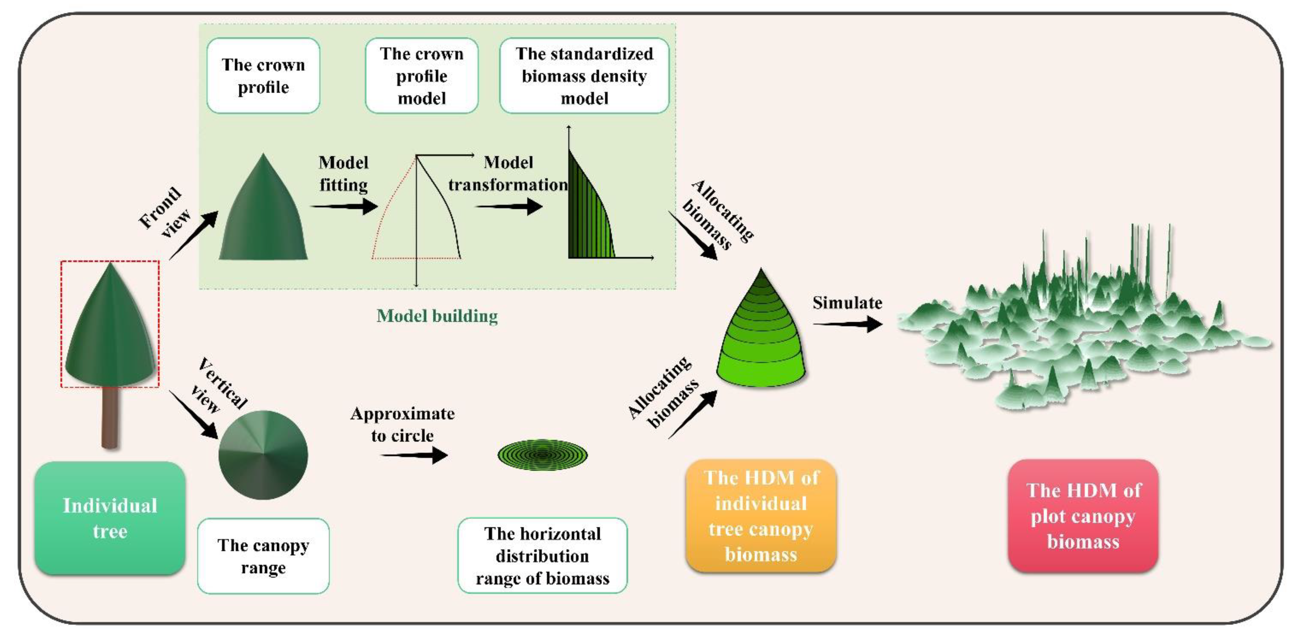
2.2.1. The Basic Idea of the HDM Construction

In this study, the individual tree biomass of Simao pine was divided into two parts: stem and crown biomass, where the crown biomass included branch and leaf biomass. The vertical projection area of the stem is small, so the difference in biomass distribution at different horizontal positions of the stem can be ignored. Therefore, the study focuses on constructing a model for the horizontal distribution of individual tree crown biomass.

For ease of study and calculation, the canopy is assumed to be a spatial geometry formed by the rotation of the outer CPM along the central axis of the stem (Figure 2). The canopy biomass is uniformly dense in the canopy space, the biomass is isotropically distributed in the horizontal plane, and all trees have the same standard distribution. The variation of the internal biomass distribution depends only on the shape variation of the outer CPM. Therefore, this study was prepared to construct a model of the profile of the individual tree canopy of Simao pine, followed by converting it into an HDM of individual tree canopy biomass. The canopy biomass distribution was combined with the trunk biomass distribution to simulate the horizontal distribution of AGB within the plot.

In this study, the canopy extent of each tree was divided into 1 cm × 1 cm rasters, and the canopy biomass was distributed according to a biomass HDM. From the center of the canopy circle, it is distributed along the radius of the canopy towards the edge of the canopy, forming several concentric circles of varying biomass. The canopy biomass distribution of each tree is then distributed within each circle. The stem biomass distribution of each tree was matched to the canopy biomass distribution to obtain the AGB horizontal distribution of each tree. Finally, the biomass distribution of all trees in the plot was superimposed on the coordinate positions to obtain the AGB distribution of the whole plot.

2.2.2. Construction of the CPM for Simao Pine

The dependent variable of the crown profile model is the crown radius (CR), and the independent variable is the relative depth into the crown (RDINC). Their calculation is shown in Equations (5) and (6), respectively. According to the relevant research [37,38,41,42], the power function, quadratic parabolic function, and logarithmic function are simple in model form, flexible, and easy to apply, and they were used to fit the CPM. The equations of the three models are shown in Equations (7)–(9), respectively.

$$\mathrm{CR}=\mathrm{BCL}·\sin \mathrm{BA}$$

(5)

$$\mathrm{RNDIC}=\left(\mathrm{DINC}-\mathrm{BCL}·\cos \mathrm{BA}\right)/\mathrm{CL}$$

(6)

$$\mathrm{CR}=\mathrm{a}·{\mathrm{RDINC}}^{\mathrm{b}}$$

(7)

$$\mathrm{CR}=\mathrm{a}+\mathrm{b}·\mathrm{RDINC}+\mathrm{c}·{\mathrm{RNDIC}}^2$$

(8)

$$\mathrm{CR}=\mathrm{a}+\mathrm{b}·\mathrm{lnRNDIC}$$

(9)

where: a, b, and c are constants.

The biomass horizontal distribution model established in this study has two aspects of error: the model fitting error on the one hand and the model prediction error on the other. Coefficient of determination (R²) and root mean square error (RMSE) were used to evaluate the model fitting error, and mean absolute error (MAE) and prediction accuracy (P) were used to evaluate the prediction error.

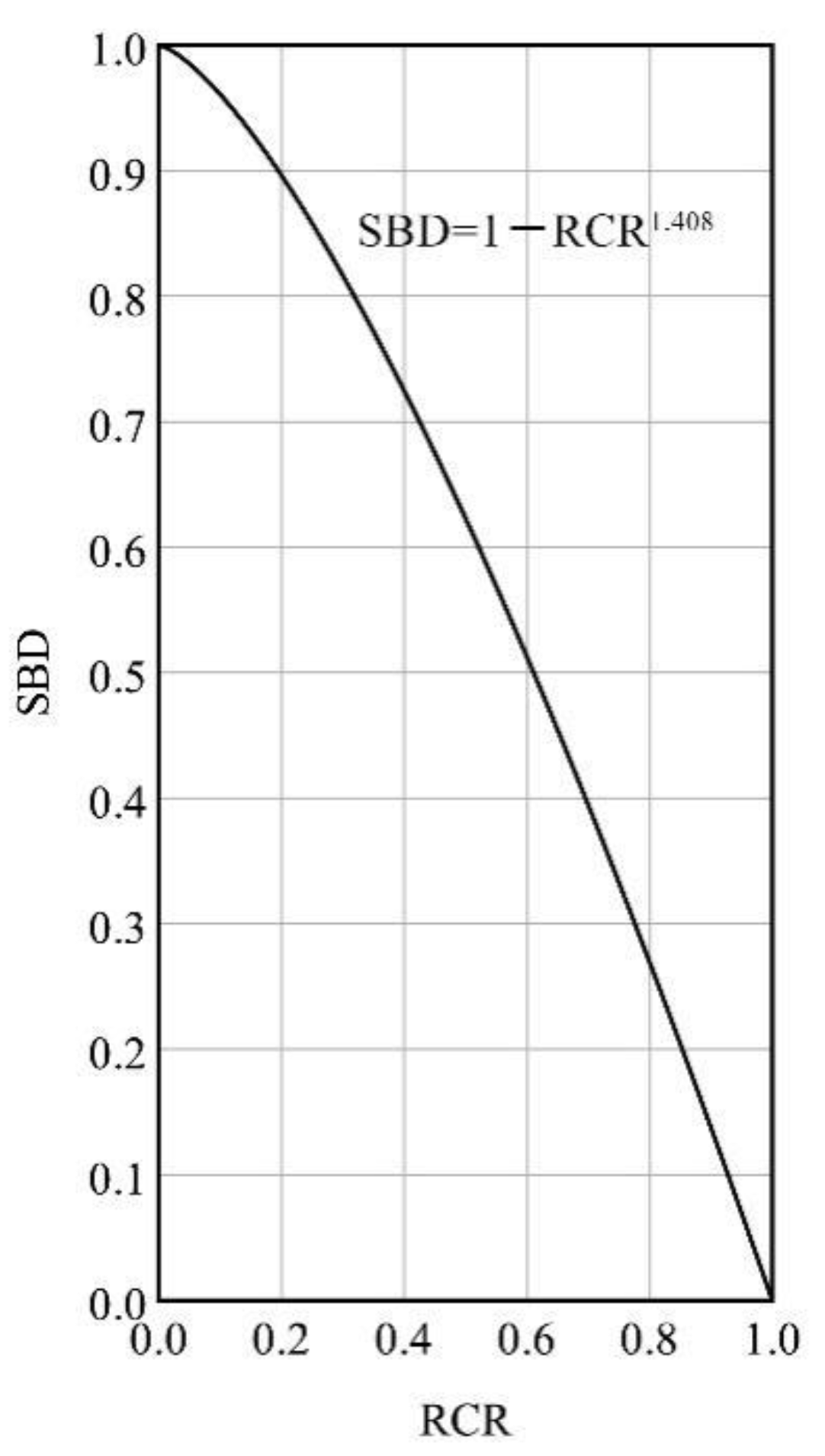
2.2.3. Construction of the HDM for the Canopy Biomass of Simao Pine

Based on the assumption that canopy biomass is distributed horizontally according to the CPM, the model (Equation (10)) needs to be converted for ease of calculation. The conversion process was as follows: the CR is converted to the relative crown radius (RCR) based on the maximum crown radius (CR_max), and the RDINC is converted to the standardized biomass density (SBD). The quantitative relationships between them are shown in Equations (11) and (12). Ultimately, an HDM of crown biomass for Simao pine, with the dependent variable being the relative radius of the crown and the independent variable being the standardized biomass density, was obtained (Equation (13)).

$$\mathrm{CR}=f\left(\mathrm{RDINC}\right)$$

(10)

$$\mathrm{RCR}=\mathrm{CR}/{\mathrm{CR}}_{\max }$$

(11)

$$\mathrm{SBD}=1-\mathrm{RDINC}$$

(12)

$$\mathrm{SBD}=f\left(\mathrm{RCR}\right)$$

(13)

2.3. Sampling Design

2.3.1. Sampling Methods

In this study, different sampling methods were combined with different biomass distribution models to form a variety of sampling schemes. The sampling method uses the simple random sampling method (SRS) and the stratified sampling method (STS). In this case, STS uses the biomass within the sampling unit as a stratification marker. The total was divided into five strata by the cumulative equivalent square root method [43,44], with random sampling within each stratum to minimize both within-stratum variance and sampling costs. According to the Technical Regulations for Continuous Forest Inventory (GB/T 38590-2020) [45], this study’s reliability index was 95%, and the sampling accuracy was set at 90%. In order to weaken the randomness of the sampling, 1000 replicate samples were taken for each data set. The sampling process was implemented through R software.

2.3.2. Sample Shape and Sample Unit Scale

In this study, the typical square shape of the sample unit is used, and ten scales of sampling units (1 m × 1 m, 2 m × 2 m, 3 m × 3 m, 4 m × 4 m, 5 m × 5 m, 6 m × 6 m, 7 m × 7 m, 8 m × 8 m, 9 m × 9 m and 10 m × 10 m) are set. Forty sampling plans were designed by combining 10 sample unit scales, two biomass distribution models, and two sampling methods. The best solution for biomass estimation was preferred by comparing different sampling plans.

2.3.3. Calculation of Sample Size

The sample size for simple random sampling is commonly calculated using Equation (14), and the sample size for stratified sampling is determined using the proportional allocation method, which is calculated using Equation (15). In practical sampling, however, calculations must be made based on the relationship between the sampled population (N) and the sample size (n). Firstly, the approximate sample size (n₀) value is calculated according to Equation (14). Secondly, the sampling ratio (f) is calculated. If the sampling ratio is less than 0.05, the difference between n₀ and n can be ignored, and the sample size is taken as n₀; otherwise, a correction is made to n₀ by Equation (16). However, in this study, the sampling range is stand scale, and there will be cases where the sampling ratio is more significant than 0.05 at different sampling unit sizes. In this case, therefore, the sample size calculation needs to be corrected using Equation (16) to improve the sampling accuracy.

$$n_0={\left(\frac{t\left(\alpha ,\mathrm{df}\right)C}{E}\right)}^2$$

(14)

$$n_0=\frac{t{\left(\alpha ,\mathrm{df}\right)}^2\sum w_h{\sigma }_h^2}{E^2{\left(\sum w_h{\overline{y}}_h\right)}^2}$$

(15)

$$n=\frac{n_0}{1+\frac{n_0}{N}}$$

(16)

where: $t\left(\alpha ,\mathrm{df}\right)$ denotes the reliability indicator, also known as probabilistic assurance, which is determined from the reliability index by which confidence intervals can be calculated with probability 1 − α; α is the critical value, which is 0.05 in this study; df is the degree of freedom, which is equal to n − 1; $w_h$ denotes the h-th strata weight; ${\sigma }_h^2$ denotes the variance of the h-th strata; C denotes the coefficient of variation; and E denotes the relative error limit.

2.3.4. Evaluation of Sampling Efficiency

Sampling efficiency needs to be evaluated in two aspects: sampling precision and sampling cost. In this study, the mean sampling estimation precision (MP), the mean relative error (MRE), and the mean coefficient of variation (MCV) were used to evaluate the sampling precision. The MP is used to assess the accuracy of sampling results. The MRE is used to evaluate the relative error of sampling results. Moreover, the MCV measures the stability of sampling results. They are calculated in Equations (17)–(19).

$$\mathrm{MP}=\frac{1}{m}{\displaystyle \sum }_{i=1}^m{P}_i$$

(17)

$$\mathrm{MRE}=\frac{1}{m}{\displaystyle \sum }_{i=1}^m\frac{\left|{\widehat{Y}}_i-Y\right|}{Y}\times 100\%$$

(18)

$$\mathrm{MCV}=\frac{1}{m}{\displaystyle \sum }_{i=1}^m\frac{\sqrt{v\left({\widehat{Y}}_i\right)}}{{\widehat{Y}}_i}\times 100\%$$

(19)

where: $P_i$ denotes the precision of the i-th sampling estimate; m denotes the number of repetitions of the sample, and m equals 1000 in this study; ${\widehat{Y}}_i$ denotes the population estimation of forest AGB for the i-th sampling; Y denotes the actual value of the overall forest AGB; and $v\left({\widehat{Y}}_i\right)$ denotes the variance of the population estimation of forest AGB for the i-th sampling.

The sample size (n) and the sampling ratio (f) were used to evaluate the sampling cost comprehensively. With the 95% reliability target and 90% sampling precision set in advance, the sampling estimation precision of 90% can theoretically be achieved for each plan. Therefore, the sampling efficiency evaluation depends primarily on the sampling cost.

3. Results

3.1. Result of the HDM Construction for the Crown Biomass of Simao Pine

The power function model, the quadratic parabolic model, and the logarithmic model were used to fit the Simao pine crown profile. The parameter estimation and model evaluation results are shown in

Table 3. The parameter estimation and model evaluation for three CPMs.

Model	Parameter Estimation			Model Fitting			Test of Independence
	a	b	c	R2	p-Value	RMSE	MAE	P (%)
Power Function	3.996	0.710	—	0.631	<0.001	0.627	0.508	66.36
Quadratic Parabolic Function	0.288	5.010	−1.338	0.628	<0.001	0.630	0.509	68.72
Logarithmic Function	2.858	0.825	—	0.541	<0.001	0.700	0.651	47.29

, and the canopy outer profile curves fitted by the three models are shown in Figure 3. As can be seen from Table 3, the R² of the power function and the quadratic parabolic model are similar and both above 0.6, which is significantly higher than that of the logarithmic function. The RMSE and MAE of the power function are the smallest among the three models, but the difference with the quadratic parabolic model is not significant. The quadratic parabola has the largest P at 68.72%, slightly higher than the power function and significantly higher than the logarithmic function. Therefore, considering the model evaluation indicators together, it can be concluded that the power function model and the quadratic parabolic model are the more effective of the three models. Among them, the power function model is slightly better. It is also clear from Figure 3 that the power function model has a CR of 0 m when RDINC is 0, which is consistent with the biological properties of the canopy. In summary, the power function model in this study was the best model for fitting the crown profile of Simao pine.

The preferred CPM was converted to the canopy biomass HDM according to the quantitative relationships in Equations (11) and (12), and the results are shown in Figure 4.

3.2. Comparison of AGB Distributions Simulated by Different Distribution Models

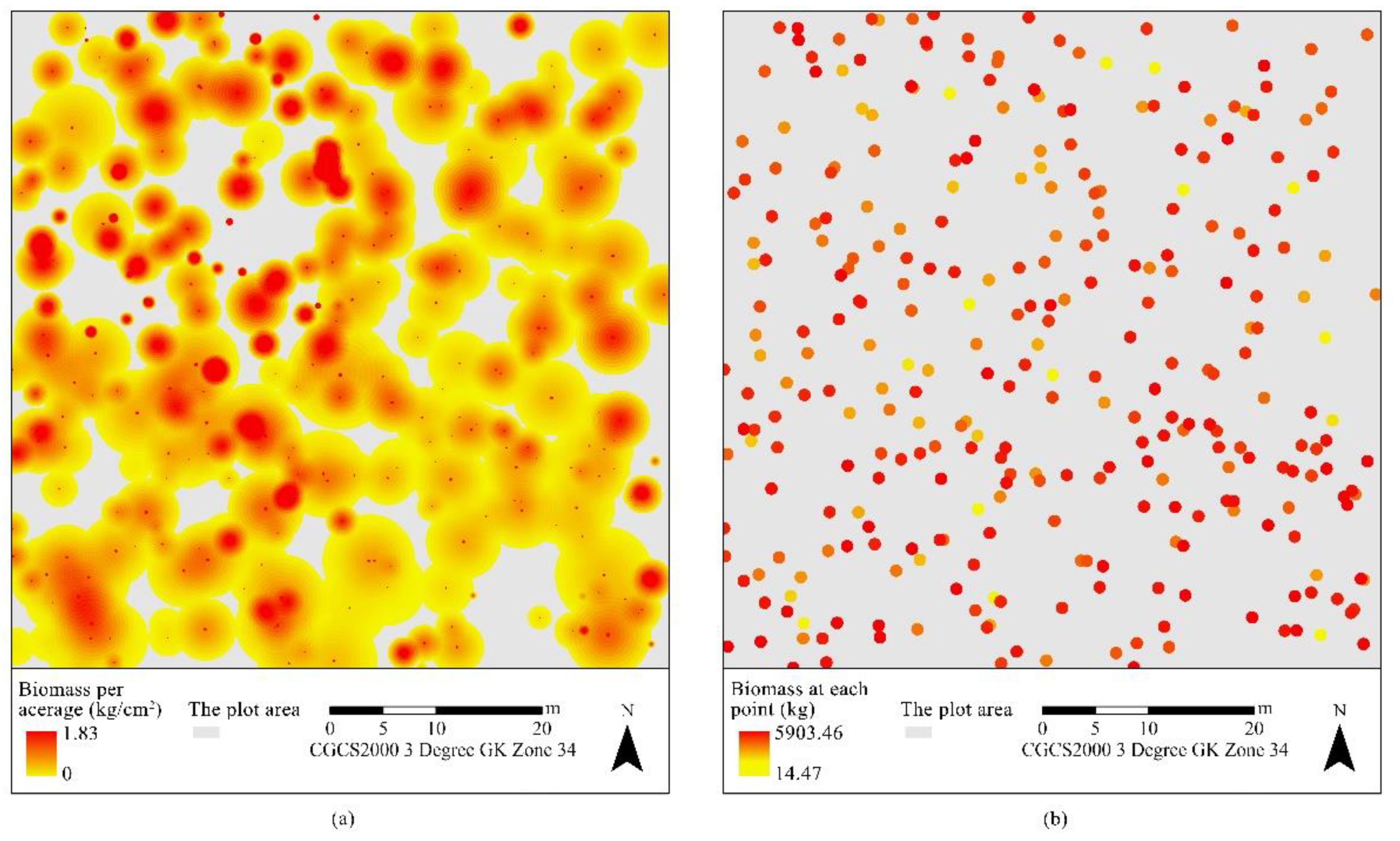
3.2.1. Visual Comparison

The AGB distribution of the plot simulated by the two biomass distribution models is shown in Figure 5. The visual comparison revealed that the AGB distribution within the HDM-based simulations was more homogeneous than that of the LDM, with a larger distribution area, continuous distribution, and less variation in biomass within adjacent ranges. However, the AGB distribution in the plot based on LDM simulation is more concentrated. The distribution area is tiny (just some points), showing sporadic distribution, and the biomass changes significantly and violently in the adjacent range. Therefore, the AGB distribution of sample plots simulated by HDM is more consistent with the biological characteristics of continuous and gradual biomass distribution of Simao pine and closer to the actual situation of plot AGB distribution.

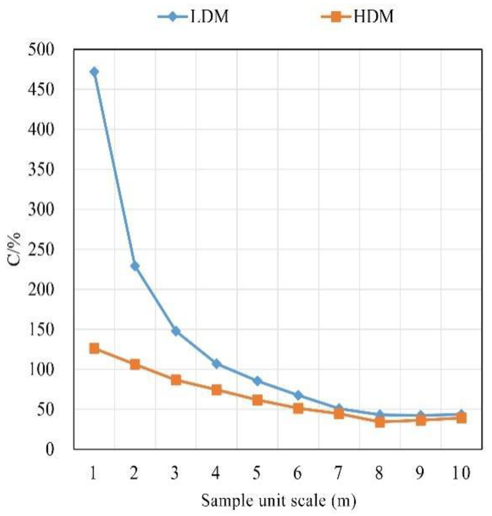
3.2.2. Analysis of Coefficients of Variation

Figure 6 shows the variation coefficient of AGB of the sample plots simulated by different biomass distribution models with the size of the sample unit. As seen in Figure 6, under the two biomass distribution models, the variation coefficient decreases with the increase in sample unit size and finally tends to be stable. Among them, the AGB variation coefficient based on the LDM distribution decreases sharply when the side length of the sample unit is 1–4 m, the decreasing trend is slightly moderate when the side length of the sample unit is 4–7 m, and it is stable at 7–10 m. The variation coefficient of AGB based on HDM distribution decreases considerably when the side length of the sample unit is 1–6 m, and the change rate is low and tends to be stable when the side length is 6–10 m. In addition, the coefficient of variation of the LDM method is always higher than that of the HDM method in the sample units of ten scales. The difference between the two is evident at 1–5 m, while the difference between the two is slight at 6–10 m. It shows that the AGB distribution based on the HDM method is more uniform in each sample unit at 1–5 m, and the advantages are apparent compared with the LDM method. However, with the increase in the scale of the sample unit, the distribution of biomass values in each sample unit tends to be consistent under the two distribution methods.

3.3. Sampling Efficiency Evaluation

3.3.1. Effect on Sample Size

Under the condition that the reliability index is 95% and the sampling accuracy is 90%, the sample sizes of four sampling schemes (SRS-HDM, STS-HDM, SRS-LDM, STS-LDM) are calculated to the variation coefficients of different sampling unit sizes. Then, the sample sizes of the two biomass distribution models are analyzed. The sample size of each scheme design is shown in Figure 7. It can be seen from Figure 7a that among the four sampling schemes, the SRS-LDM scheme has the largest sample capacity in each scale sample unit, followed by the SRS-HDM and STS-LDM schemes, and the STS-HDM scheme is the smallest. In each group of sampling plans, the sample size decreases with the increase in the size of the sample unit, which reduces significantly at 1–5 m and tends to be stable at 6–10 m. Combined with Figure 7b, we can see that when the sampling method and the scale of the sampling unit are the same, the sample size of the scheme with HDM distribution is generally smaller than that of LDM. Moreover, as the sample unit scale decreases, the saving ratio of sample size ((sample size of LDM − sample size of HDM)/sample size of LDM) increases for HDM versus LDM, up to a maximum of 89.24%. It is evident that under different sampling designs, the biomass distribution method using the HDM method can be used for a better saving of sample size.

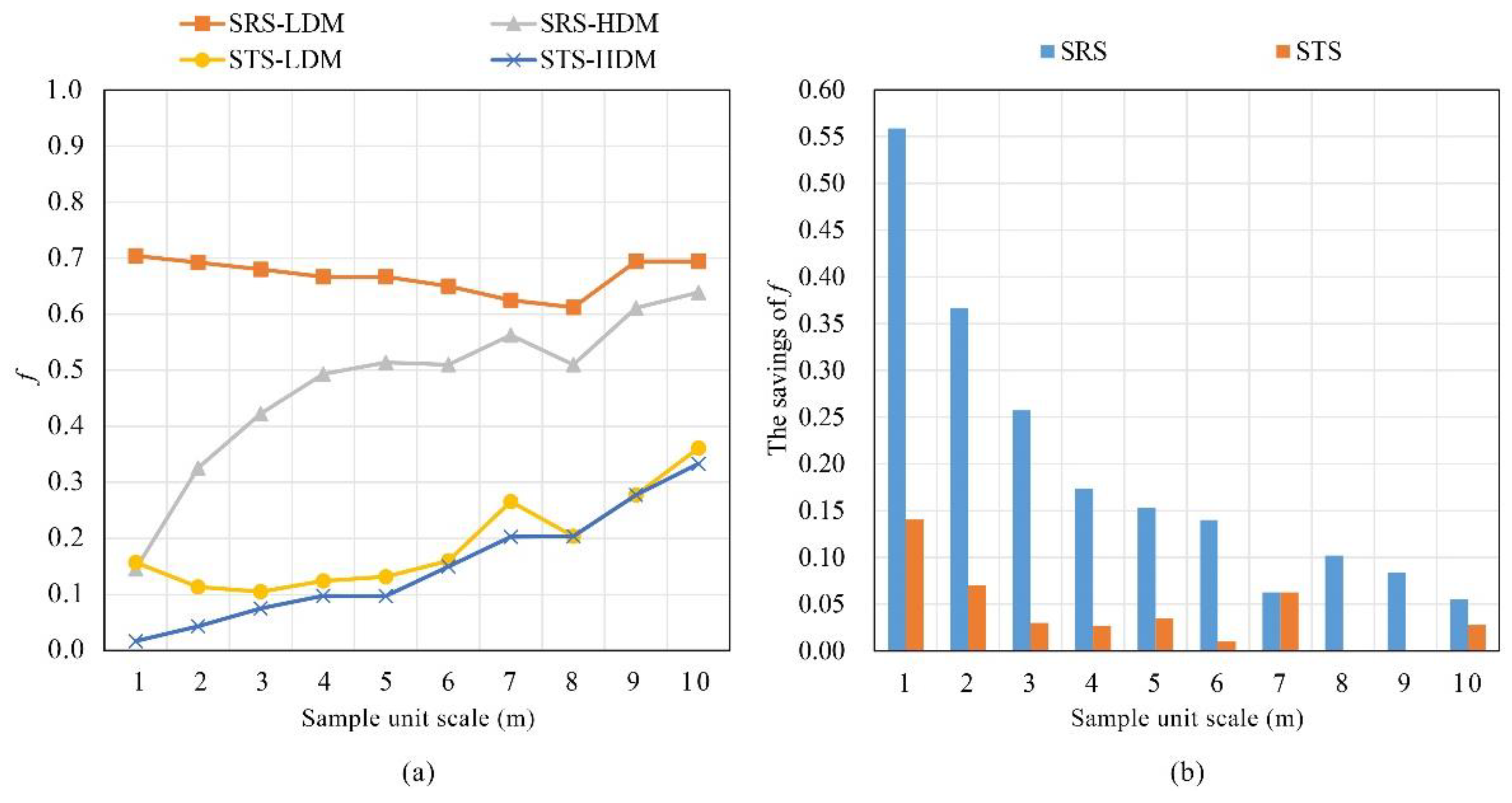
3.3.2. Effect on Sampling Ratio

The sampling ratio designed under each sampling scheme is shown in Figure 8. It can be seen from Figure 8a that under the sample units of each scale, the scheme with the highest sampling ratio is the SRS-LDM scheme, followed by the SRS-HDM and STS-LDM schemes, and the STS-HDM plan has the smallest sampling ratio. Combined with Figure 8b, it can be seen that the sampling ratio of the scheme with distribution method HDM is always smaller than that of LDM with the same sampling method and sampling unit size, and the maximum sampling ratio difference can be up to 0.56. Therefore, under different sampling designs, the biomass distribution method with HDM can effectively reduce the sampling ratio.

3.3.3. Optimization of Sampling Plans

Based on the 60 m × 60 m plot of Simao pine, different biomass distribution methods, sampling methods, and sample unit sizes were combined to form 40 various plot-scale biomass sampling schemes. Each scheme was repeated 1000 times. Their sampling efficiency evaluation indicators are shown in

Table 4. Evaluation of sampling efficiency of different biomass sampling estimation schemes.

Sample Unit Size (m)	Sample Method	Biomass Distribution	N	C (%)	Sampling Cost		Sampling Precision
					n	f	MP (%)	MRE (%)	MCV (%)
1	SRS	LDM	3600	472.05	2535	0.70	90.01	4.02	5.09
		HDM	3600	126.17	524	0.15	90.02	4.03	5.08
	STS	LDM	3600	472.05	567	0.16	91.37	3.64	4.40
		HDM	3600	126.17	61	0.02	91.15	3.65	4.42
2	SRS	LDM	900	229.22	623	0.69	89.98	4.15	5.10
		HDM	900	106.06	293	0.33	89.97	4.35	5.09
	STS	LDM	900	229.22	102	0.11	91.07	3.71	4.50
		HDM	900	106.06	39	0.04	91.52	3.50	4.18
3	SRS	LDM	400	147.85	272	0.68	89.99	3.98	5.08
		HDM	400	86.59	169	0.42	90.00	4.05	5.06
	STS	LDM	400	147.85	42	0.11	91.77	3.30	4.06
		HDM	400	86.59	30	0.08	91.70	3.36	4.03
4	SRS	LDM	225	107.03	150	0.67	90.00	4.09	5.05
		HDM	225	74.44	111	0.49	90.01	3.98	5.03
	STS	LDM	225	107.03	28	0.12	91.19	3.55	4.26
		HDM	225	74.44	22	0.10	91.65	3.38	3.96
5	SRS	LDM	144	85.42	96	0.67	89.94	4.15	5.05
		HDM	144	61.68	74	0.51	89.98	4.14	5.01
	STS	LDM	144	85.42	19	0.13	90.88	3.55	4.25
		HDM	144	61.68	14	0.10	90.98	3.19	3.99
6	SRS	LDM	100	67.40	65	0.65	90.01	4.11	4.97
		HDM	100	51.18	51	0.51	89.85	3.98	5.03
	STS	LDM	100	67.40	16	0.16	91.45	3.31	3.88
		HDM	100	51.18	15	0.15	91.66	3.34	3.74
7	SRS	LDM	64	50.89	40	0.63	89.89	4.02	4.96
		HDM	64	44.43	36	0.56	89.94	3.94	4.92
	STS	LDM	64	50.89	17	0.27	92.26	3.07	3.55
		HDM	64	44.43	13	0.20	92.24	2.92	3.37
8	SRS	LDM	49	43.01	30	0.61	89.80	3.99	4.94
		HDM	49	34.19	25	0.51	89.92	3.84	4.83
	STS	LDM	49	43.01	10	0.20	91.50	2.73	3.31
		HDM	49	34.19	10	0.20	93.56	2.11	2.50
9	SRS	LDM	36	42.34	25	0.69	90.06	3.93	4.75
		HDM	36	36.29	22	0.61	89.70	4.05	4.88
	STS	LDM	36	42.34	10	0.28	92.06	2.53	3.09
		HDM	36	36.29	10	0.28	94.25	1.81	2.24
10	SRS	LDM	36	43.57	25	0.69	89.83	3.87	4.86
		HDM	36	39.07	23	0.64	89.59	3.98	4.95
	STS	LDM	36	43.57	13	0.36	93.08	2.45	3.00
		HDM	36	39.07	12	0.33	92.43	2.86	3.20

. As can be seen in Table 4, the average sampling prediction accuracy of 40 groups of sampling plans is basically up to 90% (in the case of keeping integers), and the average relative error is less than 5%. These two indicators meet the requirements set in advance in this study. Under the LDM method and the HDM method, the coefficient of variation tends to be stable when the side length of the sample unit is greater than 6 m and 7 m, respectively.

Furthermore, according to the principle of saving sampling costs as much as possible, the most efficient sample unit size of the SRS-LDM and STS-LDM scheme in this study is 8 m, and the optimal sample unit size of the SRS-HDM and STS-HDM plan is 6 m. Among them, the sampling ratio of the scheme STS-HDM-6 m is the smallest, which is 0.15, indicating that its sampling cost is the smallest. Therefore, on the premise that the sampling accuracy meets the estimation accuracy requirements, the scheme STS-HDM-6 m is the optimal scheme.

4. Discussion

Most of the existing studies on forest biomass sampling estimation [46,47,48,49] focus on large-scale research areas, and the minimum sample unit size of these studies is generally the plot scale. However, when considering the biomass in the sample unit at the plot scale, the biomass in the sample unit is usually regarded as a whole. The detailed distribution of the biomass of individual trees in it on the horizontal plane is not considered. The refined management of forestry carbon sinks has put forward new requirements for accurately estimating forest biomass at a small scale. Sampling technology can meet its reliability requirements. Therefore, when using sampling methods to estimate forest biomass at the plot scale, it is necessary to consider the horizontal distribution of biomass of an individual tree in the sample plot.

By evaluating the sampling efficiency under different biomass distribution models, this study verified that the AGB estimation method combining HDM and sampling techniques could effectively improve the efficiency of AGB estimation in plot-scale forests. Under the condition that the preset reliability index is 95% and the sampling accuracy is 90%, the sampling accuracy of 40 sampling plans according to different sampling methods, different biomass distribution methods, and different sampling unit size combinations all meet the set requirements. Therefore, the main difference between the programs is the difference in sampling cost. It is known from each scheme’s sample size and sampling ratio contrasts that the HDM scheme offers different degrees of sampling cost-saving than that of the LDM scheme, and the smaller the sample unit, the more cost-saving. This may be since the difference in biomass among small-scale sample units based on HDM distribution is smaller than that based on LDM distribution. Under the small-scale sample unit, the sample biomass simulated by HDM is more representative of the total biomass of the sample plot than that of LDM. Therefore, using HDM to simulate the biomass distribution in the sample plot can significantly reduce the sampling cost and improve the sampling efficiency.

The model in this study was constructed based on the tree CPM. Under this distribution model, the sampling efficiency of different plans has been improved, which indicates that the horizontal distribution model of single-tree biomass based on the CPM can reflect the actual biomass distribution of single-tree biomass of Simao pine to a certain extent. The application of the CPM to describe the distribution of canopy biomass is based on a series of assumptions, such as the vertical projection of the canopy being a circle and the biomass density in the canopy space being consistent. However, these assumptions are not entirely consistent with the actual situation of the canopy biomass distribution. Therefore, to further improve the accuracy and authenticity of the horizontal distribution model of single-tree biomass, it is necessary to construct a more accurate single-tree horizontal distribution model of biomass by measuring the canopy biomass in the next step. Referring to the method of Kleinn et al. [27], the biomass distribution model of each part can be constructed according to the analysis data of tree stem, branch, and leaf and then integrated into a single-tree biomass horizontal distribution model according to the positional relationship.

In terms of modeling data acquisition, constructing a CPM model requires destructive measurements of a certain number of trees to obtain branch resolution data. In contrast, the remote sensing modeling method uses remote sensing means, such as airborne multispectral, terrestrial laser scanning, and airborne laser scanning [28], to acquire data, which can effectively avoid destroying trees and significantly improve efficiency and accuracy with tremendous potential for application [50] but may also bring problems such as rising costs. As for the type of models, this study chose parametric models for the convenience of the research. These models may only be adapted to the region and are not very generalizable. In order to improve the estimation capability of the model, machine learning methods such as support vector machine, random forest and gradient boosted regression tree [51,52,53] can be applied to the construction of biomass horizontal distribution models as a next step to further improve the robustness of the models.

5. Conclusions

This study used a 60 m × 60 m sample plot of Simao pine as the study object. The HDM of canopy biomass was constructed based on the CPM. The canopy biomass of Simao pine is allocated to the vertical projection plane of the canopy according to this model, and the distribution of stem biomass is superimposed to obtain the AGB distribution of the sample plot. The biomass distribution characteristics of different models were compared visually and by the coefficient of variation. The biomass sampling estimation scheme was optimized according to the sampling cost and accuracy. The conclusions are as follows:

(1)

The power function model is the best model to fit the contour curve of the individual tree canopy of Simao pine in this study. The CPM, based on the power function, can describe the actual distribution of the canopy biomass to a certain extent and can lay the foundation for constructing the horizontal distribution model of the individual tree biomass.

(2)

The AGB distribution of the sample plot simulated by HDM is more uniform and continuous than that of LDM, which is more in line with the actual AGB distribution of the sample plot. Under the sampling units of each scale, the difference between the AGB sampling units of the HDM-based sample plots is more negligible than that of the LDM, the sampling unit changes are more stable, and the representativeness of the total AGB of the sample plots is stronger.

(3)

The biomass estimation method combining HDM and sampling techniques proposed in this study can significantly reduce the sample size and sampling ratio, effectively improving the sampling efficiency and meeting the need for rapid, accurate, and reliable estimation of forest biomass at the sample plot scale.

References

1. Sun, W.; Liu, X. Review on Carbon Storage Estimation of Forest Ecosystem and Applications in China. For. Ecosyst. 2020, 7, 37–50. [Google Scholar] [CrossRef] [Green Version]
2. Zhao, M.; Yang, J.; Zhao, N.; Liu, Y.; Wang, Y.; Wilson, J.P.; Yue, T. Estimation of China’s Forest Stand Biomass Carbon Sequestration Based on the Continuous Biomass Expansion Factor Model and Seven Forest Inventories From 1977 to 2013. For. Ecol. Manag. 2019, 448, 528–534. [Google Scholar] [CrossRef]
3. Fang, J.; Wang, G.G.; Liu, G.; Xu, S. Forest Biomass of China: An Estimate Based on the Biomass-volume Relationship. Ecol. Appl. 1998, 8, 1084–1091. [Google Scholar]
4. Shao, G.; Shao, G.; Gallion, J.; Saunders, M.R.; Frankenberger, J.R.; Fei, S. Improving Lidar-based Aboveground Biomass Estimation of Temperate Hardwood Forests with Varying Site Productivity. Remote Sens. Environ. 2018, 204, 872–882. [Google Scholar] [CrossRef]
5. Zeng, P.; Zhang, W.; Li, Y.; Shi, J.; Wang, Z. Forest Total and Component Above-ground Biomass (AGB) Estimation Through C- and L-band Polarimetric Sar Data. Forests 2022, 13, 442. [Google Scholar] [CrossRef]
6. Zhu, Y.; Feng, Z.; Lu, J.; Liu, J. Estimation of Forest Biomass in Beijing (China) Using Multisource Remote Sensing and Forest Inventory Data. Forests 2020, 11, 163. [Google Scholar] [CrossRef] [Green Version]
7. Fang, J.; Wang, Z. Forest Biomass Estimation at Regional and Global Levels, with Special Reference to China’s Forest Biomass. Ecol. Res. 2001, 16, 587–592. [Google Scholar] [CrossRef]
8. Su, Y.; Guo, Q.; Xue, B.; Hu, T.; Alvarez, O.; Tao, S.; Fang, J. Spatial Distribution of Forest Aboveground Biomass in China_ Estimation Through Combination of Spaceborne Lidar, Optical Imagery, and Forest Inventory Data. Remote Sens. Environ. 2016, 173, 187–199. [Google Scholar] [CrossRef] [Green Version]
9. Yu, Y.; Pan, Y.; Yang, X.G.; Fan, W.Y. Spatial Scale Effect and Correction of Forest Aboveground Biomass Estimation Using Remote Sensing. Remote Sens. 2022, 14, 2828. [Google Scholar] [CrossRef]
10. Lu, D.; Chen, Q.; Wang, G.; Liu, L.; Li, G.; Moran, E. A Survey of Remote Sensing-based Aboveground Biomass Estimation Methods in Forest Ecosystems. Int. J. Digit. Earth 2016, 9, 63–105. [Google Scholar] [CrossRef]
11. Abbas, S.; Wong, M.S.; Wu, J.; Shahzad, N.; Irteza, S.M. Approaches of Satellite Remote Sensing for the Assessment of Above-ground Biomass Across Tropical Forests: Pan-tropical to National Scales. Remote Sens. 2020, 12, 3351. [Google Scholar] [CrossRef]
12. Silva, C.A.; Duncanson, L.; Hancock, S.; Neuenschwander, A.; Thomas, N.; Hofton, M.; Fatoyinbo, L.; Simard, M.; Marshak, C.Z.; Armston, J.; et al. Fusing Simulated Gedi, ICESat-2 and Nisar Data for Regional Aboveground Biomass Mapping. Remote Sens. Environ. 2021, 253, 112234. [Google Scholar] [CrossRef]
13. Vafaei, S.; Soosani, J.; Adeli, K.; Fadaei, H.; Naghavi, H.; Pham, T.D.; Bui, D.T. Improving Accuracy Estimation of Forest Aboveground Biomass Based on Incorporation of ALOS-2 PALSAR-2 and Sentinel-2A Imagery and Machine Learning: A Case Study of the Hyrcanian Forest Area (Iran). Remote Sens. 2018, 10, 172. [Google Scholar] [CrossRef] [Green Version]
14. Ou, G.; Li, C.; Lv, Y.; Wei, A.; Xiong, H.; Xu, H.; Wang, G. Improving Aboveground Biomass Estimation of Pinus densata Forests in Yunnan Using Landsat 8 imagery By Incorporating Age Dummy Variable and Method Comparison. Remote Sens. 2019, 11, 738. [Google Scholar] [CrossRef] [Green Version]
15. Chen, Q.; Laurin, G.V.; Valentini, R. Uncertainty of Remotely Sensed Aboveground Biomass Over an African Tropical Forest: Propagating Errors from Trees to Plots to Pixels. Remote Sens. Environ. 2015, 160, 134–143. [Google Scholar] [CrossRef]
16. Hill, A.; Mandallaz, D.; Langshausen, J. A Double-sampling Extension of the German National Forest Inventory for Design-based Small Area Estimation on Forest District Levels. Remote Sens. 2018, 10, 1052. [Google Scholar] [CrossRef] [Green Version]
17. Strîmbu, V.F.; Ene, L.T.; Gobakken, T.; Gregoire, T.G.; Astrup, R.; Næsset, E. Post-stratified Change Estimation for Large-area Forest Biomass Using Repeated Als Strip Sampling. Can. J. For. Res. 2017, 47, 839–847. [Google Scholar] [CrossRef] [Green Version]
18. Nelson, R.; Gobakken, T.; Næsset, E.; Gregoire, T.; Ståhl, G.; Holm, S.; Flewelling, J. Lidar Sampling—Using an Airborne Profiler to Estimate Forest Biomass in Hedmark County, Norway. Remote Sens. Environ. 2012, 123, 563–578. [Google Scholar] [CrossRef]
19. Ene, L.T.; Næsset, E.; Gobakken, T. Simulation-based Assessment of Sampling Strategies for Large-area Biomass Estimation Using Wall-to-wall and Partial Coverage Airborne Laser Scanning Surveys. Remote Sens. Environ. 2016, 176, 328–340. [Google Scholar] [CrossRef]
20. Parrott, D.L.; Lhotka, J.M.; Fei, S.; Shouse, B.S. Improving Woody Biomass Estimation Efficiency Using Double Sampling. Forests 2012, 3, 179–189. [Google Scholar] [CrossRef] [Green Version]
21. Knapp, N.; Huth, A.; Fischer, R. Tree Crowns Cause Border Effects in Area-based Biomass Estimations from Remote Sensing. Remote Sens. 2021, 13, 1592. [Google Scholar] [CrossRef]
22. Kershaw, J.A.; Maguire, D.A. Crown Structure in Western Hemlock, Douglas-Fir, and Grand Fir in Western Washington: Trends in Branch-Level Mass and Leaf Area. Can. J. For. Res. 1996, 25, 1897–1912. [Google Scholar] [CrossRef]
23. Xu, M.; Harrington, T.B. Foliage Biomass Distribution of Loblolly Pine as Affected by Tree Dominance, Crown Size, and Stand Characteristics. Can. J. For. Res. 1998, 28, 887–892. [Google Scholar] [CrossRef]
24. Nielsen, C.C.N.; Mackenthum, G. Die horizontale Varia-tion der Feinwurzelintensität in Waldböden in Abhängigkeit vonder Bestockungsdichte. Einerechnerische Methode zur Bestimmung der “Wurzelintensitätsglocke” an Einzelbäumen. Allg. Forst Und Jagdztg. 1991, 162, 112–119. [Google Scholar]
25. Fehrmann, L.; Kuhr, M.; von Gadow, K. Zur Analyse Der Grobwurzelsysteme Großer Waldbäume and Fichte [Picea abies (L.) Karst.] Und Buche [Fagus sylvatica L.] (In German: “Analyis of the Coarse Root Systems of Large Trees at Spruce [Picea abies (L.) Karst.] and Beech [Fagus sylvatica L.]”). Forstarchiv 2003, 74, 96–102. [Google Scholar]
26. Mascaro, J.; Detto, M.; Asner, G.P.; Muller-Landau, H.C. Evaluating Uncertainty in Mapping Forest Carbon with Airborne LiDAR. Remote Sens. Environ. 2011, 115, 3770–3774. [Google Scholar] [CrossRef]
27. Kleinn, C.; Magnussen, S.; Nölke, N.; Magdon, P.; Álvarez-gonzález, J.G.; Fehrmann, L.; Pérez-cruzado, C. Improving Precision of Field Inventory Estimation of Aboveground Biomass Through an Alternative View on Plot Biomass. For. Ecosyst. 2020, 7, 760–769. [Google Scholar] [CrossRef]
28. Pérez-cruzado, C.; Kleinn, C.; Magdon, P.; Álvarez-gonzález, J.G.; Magnussen, S.; Fehrmann, L.; Nölke, N. The Horizontal Distribution of Branch Biomass in European beech: A Model Based on Measurements and TLS based Proxies. Remote Sens. 2021, 13, 1041. [Google Scholar] [CrossRef]
29. Carvalho, J.P.; Parresol, B.R. Additivity in Tree Biomass Components of Pyrenean Oak (Quercus pyrenaica Willd.). For. Ecol. Manag. 2003, 179, 269–276. [Google Scholar] [CrossRef]
30. Stenberg, P.; Kuuluvainen, T.; Kellomäki, S.; Grace, J.C.; Jokela, E.J.; Gholz, H.L. Crown Structure, Light Interception and Productivity of Pine Trees and Stands. Ecol. Bull. 1994, 43, 20–34. [Google Scholar]
31. Kellomäki, S. A Model for the Relationship between Branch Number and Biomass in Pinus Sylvestris Crowns and the Effect of Crown Shape and Stand Density on Branch and Stem Biomass. Scand. J. For. Res. 1986, 1, 455–472. [Google Scholar] [CrossRef]
32. Wang, D.; Yang, L.; Shi, C.; Li, S.; Tang, H.; He, C.; Cai, N.; Duan, A.; Gong, H. QTL Mapping for Growth-related Traits By Constructing the first Genetic Linkage Map in Simao Pine. BMC Plant Biol. 2022, 22, 48. [Google Scholar] [CrossRef] [PubMed]
33. Ou, G.; Wang, J.; Xu, H.; Chen, K.; Zheng, H.; Zhang, B.; Sun, X.; Xu, T.; Xiao, Y. Incorporating Topographic Factors in Nonlinear Mixed-effects Models for Aboveground Biomass of Natural Simao Pine in Yunnan, China. J. For. Res. 2016, 27, 119–131. [Google Scholar] [CrossRef]
34. Zhu, L.M.; Xu, H. Study on Single Biomass Model for Pinus kesiya var. langbianensis. For. Sci. Technol. 2009, 34, 19–23. [Google Scholar]
35. Zhou, L.; Ou, G.L.; Wang, J.F.; Xu, H. Light Saturation Point Determination and Biomass Remote Sensing Estimation of Pinus kesiya var. langbianensis Forest Based on Spatial Regression Models. Sci. Silvae Sin. 2020, 56, 38–47. [Google Scholar]
36. Ou, G.; Xiao, Y.; Wang, J.; Xu, H.; Liu, Z. Modeling Tree Crown Structure of Simao Pine (Pinus kesiya var. langbianensis) Natural Forest. Acta Ecol. 2014, 34, 1663–1671. [Google Scholar]
37. Gao, H.; Bi, H.; Li, F. Modelling Conifer Crown Profiles as Nonlinear Conditional Quantiles: An Example with Planted Korean Pine in Northeast China. For. Ecol. Manag. 2017, 398, 101–115. [Google Scholar] [CrossRef]
38. Sun, Y.; Gao, H.; Li, F. Using Linear Mixed-effects Models with Quantile Regression to Simulate the Crown Profile of Planted Pinus Sylvestris Var. Mongolica Trees. Forests 2017, 8, 446. [Google Scholar] [CrossRef] [Green Version]
39. Baldwin, V.C.; Peterson, K.D. Predicting the Crown Shape of Loblolly Pine Trees. Can. J. For. Res. 1997, 27, 102–107. [Google Scholar] [CrossRef]
40. LY/T 2908—2017; Regulations for Age-Class and Age-Group Division of Main Tree-Species. Chinese National Technical Committee for the Standardization of Forest Resources, Standards Press of China: Beijing, China, 2017.
41. Dong, C.; Wang, C.; Wu, B.; Guo, Y.; Han, Y. Study on Crown Profile Models for Chinese Fir (Cunninghamia lanceolata) in Fujian Province and Its Visualization Simulation. Scand. J. For. Res. 2016, 31, 302–313. [Google Scholar] [CrossRef]
42. Gao, H.; Dong, L.; Li, F. Modeling Variation in Crown Profile with Tree Status and Cardinal Directions for Planted Larix olgensis Henry Trees in Northeast China. Forests 2017, 8, 139. [Google Scholar] [CrossRef] [Green Version]
43. Wang, D.; Zhou, Q.; Yang, P.; Zhong, X. Design of a Spatial Sampling Scheme Considering the Spatial Autocorrelation of Crop Acreage Included in the Sampling Units. J. Integr. Agric. 2018, 17, 2096–2106. [Google Scholar] [CrossRef]
44. Wang, D.; Li, Z.; Zhou, Q.; Yang, P.; Chen, Z. An Optimized Two-stage Spatial Sampling Scheme for Winter Wheat Acreage Estimation Using Remotely Sensed Imagery. Int. J. Remote Sens. 2018, 40, 2014–2033. [Google Scholar] [CrossRef]
45. GB/T 38590—2020; Technical Regulations for Continuous Forest Inventory. Chinese National Technical Committee for the Standardization of Forest Resources, Standards Press of China: Beijing, China, 2020.
46. Andersena, H.; Breidenbach, J. Statistical Properties of Mean Stand Biomass Estimators in a Lidar-based Double Sampling Forest Survey Design. Int. Arch. Photogramm. Remote Sens. Spat. Inf. Sci. 2007, 36, 8–13. [Google Scholar]
47. Hawbaker, T.J.; Keuler, N.S.; Lesak, A.A.; Gobakken, T.; Contrucci, K.; Radeloff, V.C. Improved Estimates of Forest Vegetation Structure and Biomass with a Lidar-optimized Sampling Design. J. Geophys. Res. Atmos. 2009, 114, G00E04. [Google Scholar] [CrossRef]
48. Næsset, E.; Gobakken, T.; Bollandsås, O.M.; Gregoire, T.G.; Nelsonc, R.; Ståhl, G. Comparison of Precision of Biomass Estimates in Regional field Sample Surveys and Airborne Lidar-assisted Surveys in Hedmark County, Norway. Remote Sens. Environ. 2013, 130, 108–120. [Google Scholar] [CrossRef] [Green Version]
49. Ståhl, G.; Holm, S.; Gregoire, T.G.; Gobakken, T.; Næsset, E.; Nelson4, R. Model-based Inference for Biomass Estimation in a Lidar Sample Survey in Hedmark County, Norway. Can. J. For. Res. 2011, 41, 96–107. [Google Scholar] [CrossRef] [Green Version]
50. Wirasatriya, A.; Pribadi, R.; Iryanthony, S.B.; Maslukah, L.; Sugianto, D.N.; Helmi, M.; Ananta, R.R.; Adi, N.S.; Kepel, T.L.; Ati, R.N.A.; et al. Mangrove Above-Ground Biomass and Carbon Stock in the Karimunjawa-Kemujan Islands Estimated from Unmanned Aerial Vehicle-Imagery. Sustainability 2022, 14, 706. [Google Scholar] [CrossRef]
51. López-Serrano, P.M.; Domínguez, J.L.C.; Corral-Rivas, J.J.; Jiménez, E.; López-Sánchez, C.A.; Vega-Nieva, D.J. Modeling of Aboveground Biomass with Landsat 8 OLI and Machine Learning in Temperate Forests. Forests 2020, 11, 11. [Google Scholar] [CrossRef] [Green Version]
52. Chen, L.; Wang, Y.; Ren, C.; Zhang, B.; Wang, Z. Assessment of Multi-Wavelength SAR and Multispectral Instrument Data for Forest Aboveground Biomass Mapping Using Random Forest Kriging. For. Ecol. Manag. 2019, 447, 12–25. [Google Scholar] [CrossRef]
53. Zhang, J.; Lu, C.; Xu, H.; Wang, G. Estimating Aboveground Biomass of Pinus densata-Dominated Forests Using Landsat Time Series and Permanent Sample Plot Data. J. For. Res. 2019, 30, 1689–1706. [Google Scholar] [CrossRef]
Figure 1. The location distribution of Simao pines in the plot. The tree icons’ different sizes indicate the DBH’s relative size.
Forests 13 01612 g001
Figure 2. Simulation process of horizontal distribution of canopy biomass in the plot.
Forests 13 01612 g002
Figure 3. Fitting curves of three CPMs. (a) Power function; (b) quadratic parabolic function; (c) logarithmic function. RDINC is the relative depth into the crown; and CR is the crown radius.
Forests 13 01612 g003
Figure 4. The HDM of canopy biomass. SBD is the standardized biomass density; and RCR is the relative crown radius.
Forests 13 01612 g004
Figure 5. The AGB distributions in the plot simulated by different distribution models of biomass. (a) Simulated by HDM; and (b) simulated by LDM.
Forests 13 01612 g005
Figure 6. Trends of the coefficient of variation for AGB under different models.
Forests 13 01612 g006
Figure 7. Effects of different biomass distribution models on the sample size. (a) Variation of sample size; and (b) The savings in the sample size of the HDM method schemes compared to the LDM method schemes.
Forests 13 01612 g007
Figure 8. Effect of different biomass sampling estimation schemes on sampling ratios. (a) Variation of sampling ratio; and (b) the savings in sampling ratio of the HDM method schemes compared to the LDM method schemes.
Forests 13 01612 g008