
Occurrence Prediction of Pine Wilt Disease Based on CA–Markov Model

1
Beijing Key Laboratory of Precision Forestry, Forestry College, Beijing Forestry University, Beijing 100083, China
2
Key Laboratory of Forest Cultivation and Protection, Ministry of Education, Beijing Forestry University, Beijing 100083, China
*
Author to whom correspondence should be addressed.
Forests 2022, 13(10), 1736; https://doi.org/10.3390/f13101736
Submission received: 27 September 2022
/
Revised: 17 October 2022
/
Accepted: 17 October 2022
/
Published: 20 October 2022
(This article belongs to the Topic Challenges, Development and Frontiers of Smart Agriculture and Forestry)
Abstract
:Pine wilt disease (PWD) has become a devastating disease that impacts China’s forest management. It is of great significance to accurately predict PWD on a geospatial scale to prevent its spread. Using the Cellular Automata (CA)–Markov model, this study predicts the occurrence area of PWD in Anhui Province in 2030 based on PWD-relevant factors, such as weather, terrain, population, and traffic. Using spatial autocorrelation analysis, direction analysis and other spatial analysis methods, we analyze the change trend of occurrence data of PWD in 2000, 2010, 2020 and 2030, reveal the propagation law of PWD disasters in Anhui Province, and warn for future prevention and control direction and measures. The results show the following: (1) the overall accuracy of the CA–Markov model for PWD disaster prediction is 93.19%, in which the grid number accuracy is 95.19%, and the Kappa coefficient is 0.65. (2) In recent 20 years and the next 10 years, the occurrence area of PWD in Anhui Province has a trend of first decreasing and then increasing. From 2000 to 2010, the occurrence area of disasters has a downward trend. From 2010 to 2020, the disaster area has increased rapidly, with an annual growth rate of 140%. In the next 10 years, the annual growth rate of disasters will slow down, and the occurrence area of PWD will reach 270,632 ha. (3) In 2000 and 2010, the spatial aggregation and directional distribution characteristics of the map spots of the PWD pine forest were significant. In 2020 and 2030, the spatial aggregation is still significant after the expansion of the susceptible area, but the directional distribution is no longer significant. (4) The PWD center in Anhui Province shows a significant trend of moving southward. From 2010 to 2020, the PWD center moved from Chuzhou to Anqing. (5) PWD mainly occurs in the north slope area below 700 m above sea level and below 20° slope in Anhui Province. The prediction shows that the PWD disaster will break through the traditional suitable area in the next 10 years, and the distribution range will spread to high altitude, high slope, and sunny slope. The results of this study can provide scientific support for the prevention and control of PWD in the region and help the effective control of PWD in China.
1. Introduction
PWD is caused by the pinewood nematode Bursaphelenchus xylophilus, known as the “cancer” of pine trees (Pinus spp.), and is the most dangerous and destructive disease in the forest ecosystem in China and Southeast Asia. It has strong diffusivity and destructiveness and is one of the diseases that causes the most significant forestry losses in China [1]. It is presumed that PWD originated in North America and was spread to Japan in the early 20th century, and it is now outbreaking in pine forests around the world [2]. China quarantined PWD for the first time in Nanjing in 1982, and PWD has since infested 19 provinces, which has caused direct economic losses and ecological service value losses of up to hundreds of billions of yuan in the past 40 years [3,4]. PWD has become a major threat to China’s ecological security, biosafety, and economic development. It is significant for disaster prevention, control, and loss reduction to carry out fine-grained PWD area prediction and early warning of PWD in large areas.
The growth and development of pests and disease pathogens relate to their living environment. The traditional pest and disease prediction mainly use their life history rhythm dependence on meteorological elements. For example, disasters can occur when environmental elements such as temperature, precipitation, or humidity meet the developmental conditions of pests or pathogens. Researchers have predicted the probability and area of disasters according to the measured or predicted environmental element data [5,6,7,8]. With the increasing trend of global warming, climate change causes a series of chain reactions such as temperature, precipitation, and humidity, which will have a direct impact on the distribution of vegetation [9,10], and indirectly affects pest pathogens and invasive plants by affecting harmful species such as insects that inhabit the vegetation. Therefore, it is becoming increasingly difficult to predict pest outbreaks based on traditional methods using only meteorological elements [10,11,12,13,14,15,16]. In order to cope with the uncertainty challenge of climate change on the prediction of vegetation diseases and insect pests, niche models [17,18,19,20] and machine learning models [21,22,23,24,25,26,27,28] have been used to predict the spatial and temporal prediction of vegetation diseases and insect pests in multi-situation and multi-factor conditions and satisfactory accuracy has been obtained.
PWD prediction has received more and more attention because it can effectively guide disaster prevention and formulate preventive measures in advance. Using satellite or unmanned aerial vehicle remote sensing data to identify the diseased trees in the early stage of PWD infection at the regional or individual scale and mapping the distribution of the infected trees can achieve early disease control [29,30]. However, this is still an overly passive and less effective early intervention. According to the influencing factors of PWD infection and transmission, it is an effective early warning and control method to predict the possible infection area [31]. This method can let people know the possible occurrence area of the disease earlier, and help the forestry management department to formulate the disease prevention and control measures in advance, so as to avoid more pine trees being destroyed. Based on traditional climate predictions, PWD is mainly concentrated in eastern and southern China, with the colder north being less suitable for its life [32]. However, according to the Chinese government’s monitoring data, the epidemic area of pine wilt nematode disease has developed in Jilin and Liaoning provinces in northern China, with the northernmost point located in Kaiyuan, Tieling, Liaoning Province [4]. Therefore, it is difficult to accurately predict the habitat of pests only by using the prediction method of meteorological elements. At present, the CART model [33,34], CLIMEX model [35,36], evapotranspiration model [37], climate scenario simulation [38,39], spatiotemporal network model [40,41], MaxEnt model [42,43], random forest model [31], spatially explicit model [44], disaster spread model [45,46,47,48] and other methods [49,50,51] are mainly used to predict PWD based on meteorological and habitat factors to predict and simulate the disaster-prone areas. However, due to less consideration of biological and human factors, obtaining superior simulation accuracy and guiding PWD prevention and control is challenging.
This research primarily concentrates on disease mechanism, the interaction between nematodes and vector beetles, ecological impact, prevention strategies, risk area based on meteorological components, and habitat prediction—biological, natural, and human activity all impact PWD catastrophes. As a result, it is currently a significant problem that needs to be solved, and it will also be the primary focus of PWD research in the future The objectives of this study are the following: (1) based on the field survey data collected by forestry patches in Anhui Province in 2000, 2010, and 2020, the CA–Markov model will be used to predict the occurrence of PWD in Anhui Province in 2030; (2) to analyze the occurrence, distribution, and characteristics of the disease in these four periods. This study is of great significance to grasp the spatio-temporal distribution, change the law, and future development trend of PWD in Anhui Province, scientifically and effectively carry out epidemic prevention and control, reduce the risk of epidemic spread and reduce the losses caused by disasters.
2. Materials and Methods
2.1. Study Area
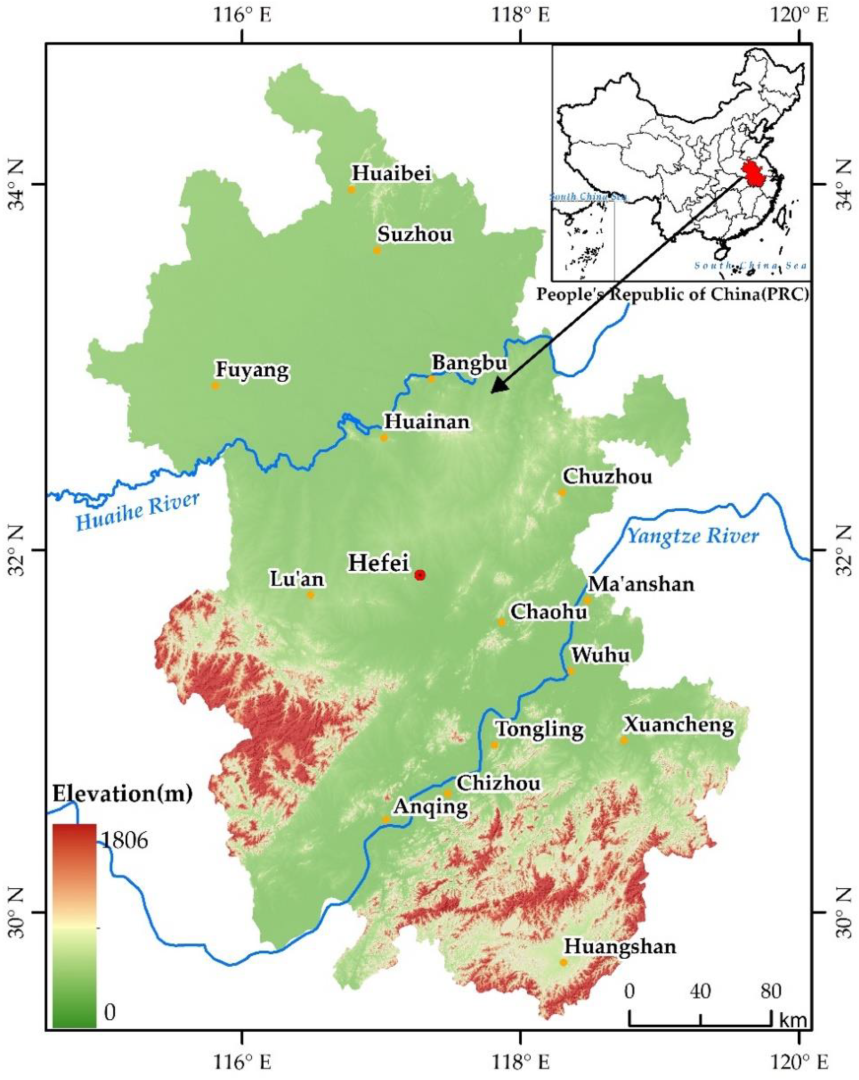
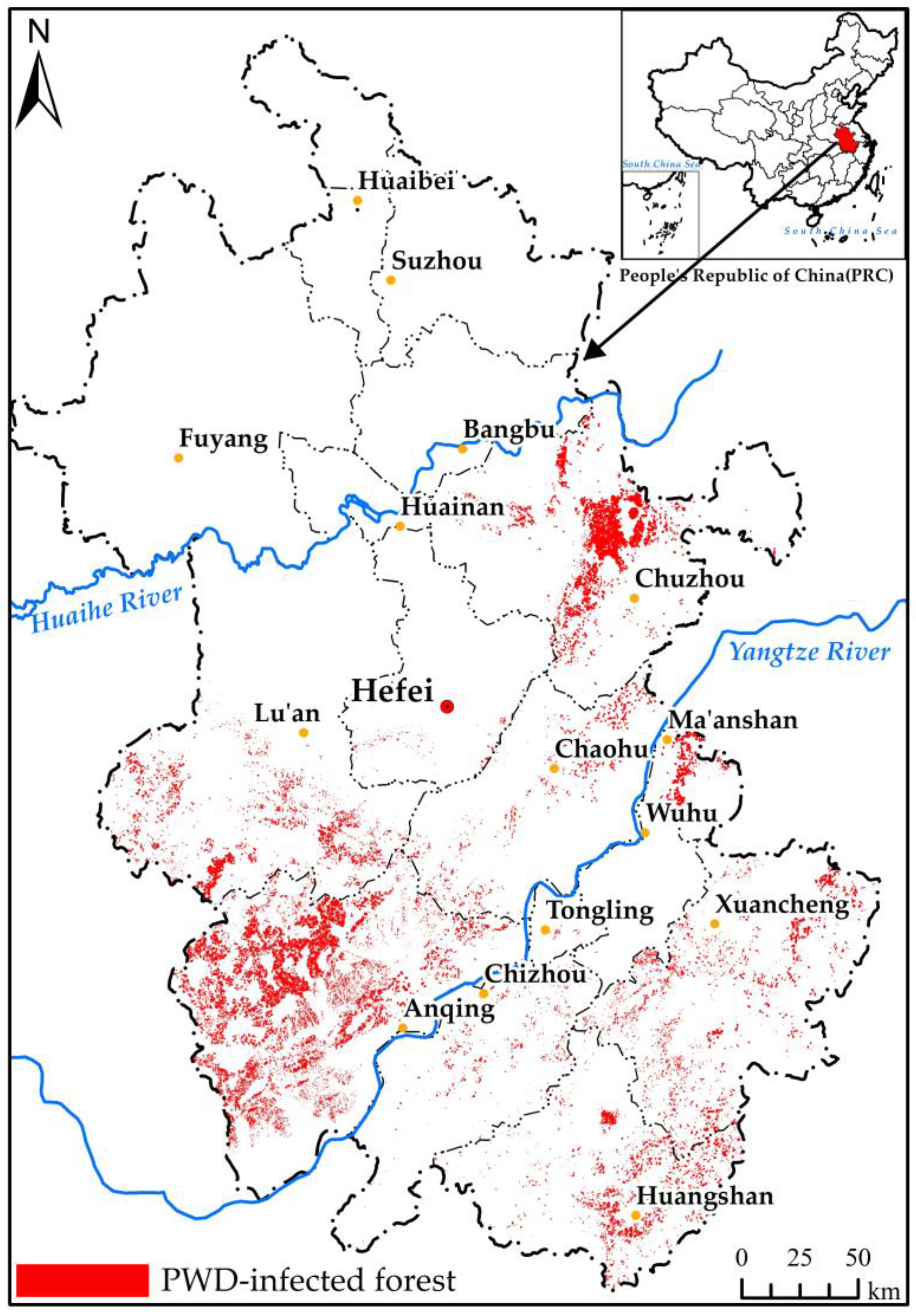
Anhui is located in East China, belonging to the lower reaches of the Yangtze River economic belt and the hinterland of the Yangtze River Delta. Its geographical location is 114°54′–119°37′ E and 29°41′–34°38′ N, with a total area of 140,100 km2. In terms of climate, it belongs to the transitional area between warm temperate zone and subtropical zone. The north of Huaihe River belongs to warm temperate zone semi-humid monsoon climate, and the south of Huaihe River belongs to sub-hot-humid monsoon climate. The annual frost-free period is 200–250 days, the accumulated temperature above 10 °C is 4600–5300 °C, the annual average temperature is 14–17 °C, and the annual average precipitation is 800–1800 mm, which is characterized by more in the south and less in the north, and more in the mountains and less in the plains and hills (Figure 1). The province has a forest area of 4.17 × 10⁶ ha, with a forest coverage rate of 30.22%.
PWD was first discovered in Anhui Province in 1988. As the environmental conditions in Anhui Province are very suitable for the prevalence and spread of PWD, there is a widespread distribution of PWD in Anhui Province. By the end of 2020, the total area of PWD is 99,603 ha, and 77.01 × 10⁴ infected pines are found in Anhui Province.
2.2. Data Acquisition
2.2.1. Distribution of Pine Forest and PWD Data
The data on the distribution of pine forests and the occurrence of PWD of Anhui Province are vector data at chart patch level, which are from the field survey of counties summarized by the Anhui Forestry Administration in 2000, 2010 and 2020, respectively, and the data format is shapefile (Figure 2). These data are used for the risk forecast of the occurrence of PWD of Anhui Province.
2.2.2. Normalized Vegetation Index (NDVI)
NDVI comes from Google Earth Engine (GEE) platform (https://earthengine.google.com) (accessed on 4 February 2021) Landsat5 and Landsat-8 OLI 32-Day data have a spatial resolution of 30 m and a temporal resolution of 32 d. The time of pine tree discoloration caused by PWD in the study area is from November of the current year to February of the next year. Therefore, the NDVI data collected the average number of November and December of the current year in 2000, 2010 and 2020, and January and February of the next year.
2.2.3. DEM
DEM comes from Geospatial Data Cloud (https://www.gscloud.cn/) (accessed on 4 February 2021) ASTER GDEM V3 product. The spatial resolution is 30 m, and the data format is TIFF.
2.2.4. Meteorological Data
The raster data of meteorological elements are derived from the monthly climate and water balance dataset of the global land surface (TerraClimate). The spatial resolution of the raster is 5000 m, the temporal resolution is month, and the data format is TIFF. The meteorological data include the monthly average wind speed, monthly maximum temperature, and monthly accumulated rainfall in 2000, 2010, and 2020. The data of sunshine hours come from National Meteorological Information Center (http://data.cma.cn/) (accessed on 4 February 2021), using the Kriging difference method to obtain the raster data, and then calculate the meteorological data of each county. Since the short-distance transmission of PWD mainly depends on the vector insect Monochamus alternatus Hope (Coleoptera Cerambycidae) (Japanese pine sawyer beetle) [52], the dormancy period of Monochamus alternatus Hope is from October of the current year to March of the next year [53]; therefore, the mean value of each meteorological factor from April to September of each year is taken as the explanation factor of meteorological elements in this study. In order to keep consistent with the spatial resolution of land use data and NDVI data in the study area, the spatial resolution of meteorological data grid is uniformly resampled to 30 m.
2.2.5. Population Distribution Data
Population and GDP distribution data comes from Global Change Research Data Publishing & Repository (http://www.geodoi.ac.cn/) (accessed on 4 February 2021), with a collection cycle of every five years. The nationwide grid data of 2000, 2010 and 2020 are obtained, respectively. The grid spatial resolution is 1 km, and the data format is TIFF. The Anhui Provincial boundary is used to cut the grid, and the spatial resolution of the grid is resampled to 30 m to be consistent with NDVI.
2.2.6. Road Distribution Data
Road distribution data comes from the Geographic Data Platform of College of Urban and Environmental Science, Peking University (http://geodata.pku.edu.cn) (accessed on 4 February 2021), the data format is shapefile, including national roads, provincial roads, county roads, township roads, expressways, railways, and urban level-1, level-2, level-3, and level-4 roads. The collected time is 2000, 2010 and 2020, respectively.
2.3. Methodology
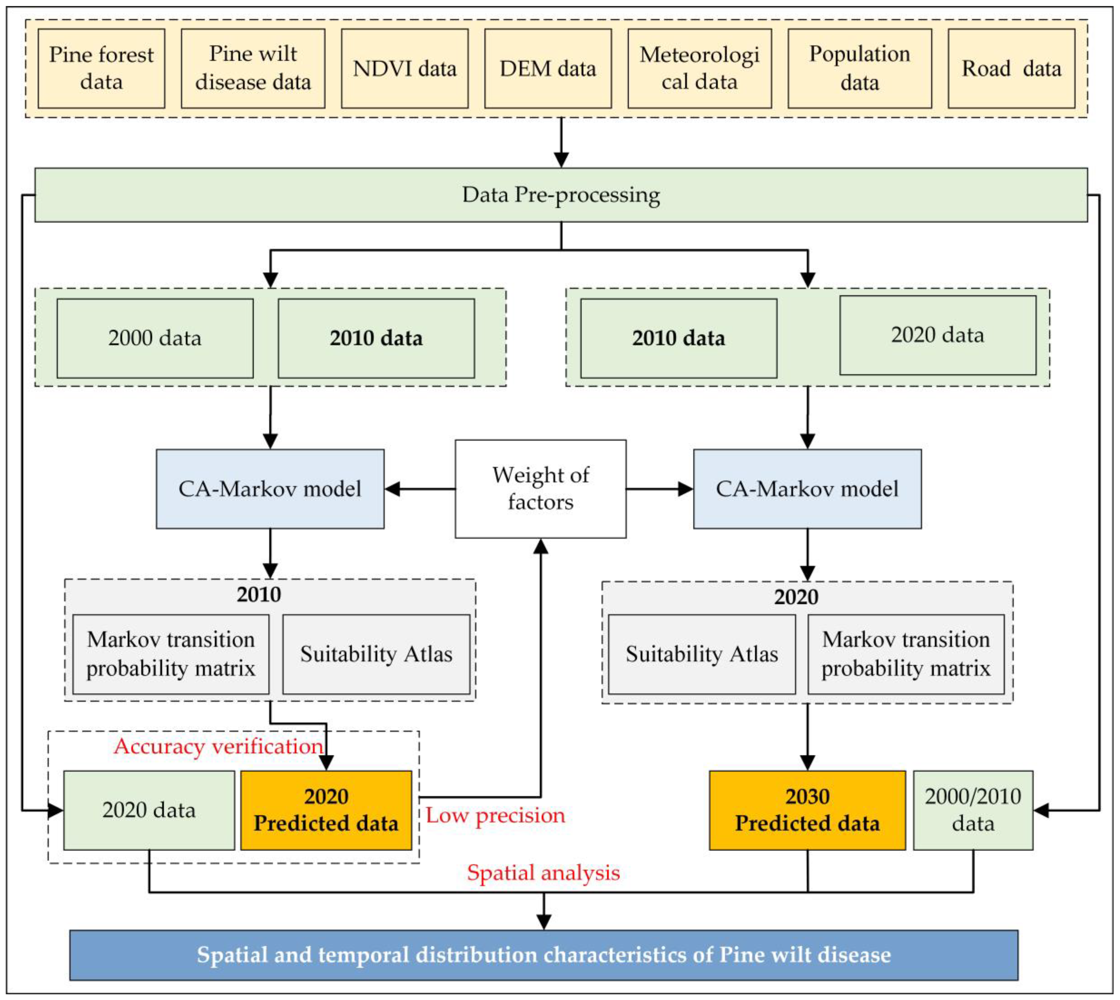
In this study, CA–Markov model is used to predict the occurrence of PWD in Anhui Province, and spatial analysis method is used to analyze the spatial and temporal distribution. The overall technical roadmap is shown in Figure 3 and Figure S1. Firstly, Markov transformation and multi-criteria evaluation (MCE) were carried out by using the patch data (grid) of pine forest and PWD disasters in 2000 and 2010, to obtain the disaster transfer (change) area, probability matrix and the suitability atlas of PWD prediction in 2000 and 2010, in Anhui Province. Secondly, CA–Markov prediction is used to obtain the prediction map of PWD occurrence in 2020. The grid quantity accuracy and Kappa coefficient accuracy of the prediction map are verified by using the patch data (grid) of pine forest and PWD disaster occurrence in 2020 and the field survey data. If the accuracy is low (Kappa < 0.4), the influencing factors and weights of PWD occurrence need to be re-evaluated, and the above two steps should be repeated. If the accuracy meets the actual application requirements, it shall be considered that CA–Markov model can be used to predict the occurrence of PWD, and the influencing factors and weights of PWD are reasonable, which can be used to predict the next decade (2030). Thirdly, based on the patch data (grid) of pine forest and PWD disasters in 2010 and 2020, Markov transformation and MEC evaluation are also carried out to obtain the suitability atlas of PWD prediction in 2020, then Markov transfer (change) area and probability matrix are conducted, respectively, and further, CA–Markov prediction is used to obtain the prediction map of PWD occurrence in 2030; Finally, the spatial analysis of the occurrence data of PWD in the four periods (2000, 2010, 2020 and 2030) is carried out to reveal the propagation law of the disaster in Anhui Province and warn the future prevention and control direction and measures.
2.3.1. CA–Markov Model
CA model is a spatiotemporal dynamic simulation model based on discontinuity, which is generated by some very simple local rules [54]. CA system generally includes four elements [55], i.e., unit, state, neighborhood range and conversion rule, whose formula is:
where S is the state set of discrete and finite units (i.e., cells), N is the neighborhood of cells, t and t + 1 represent two different moments, and f is the cell state conversion rule.
Markov model is a model to study the probability of things changing from one state to another with the relevant knowledge of probability theory, and predict the future state of things. The model focuses on the prediction of future quantity.
where St + 1 is the state of things in the moment of t + 1, St is the state of things in the moment of t, and Pij is the probability that a thing changes from one state to another.
CA–Markov model: The prediction of the random change state of Markov model is mainly a quantitative prediction, not spatial prediction; CA model has the concept of spatial information and the ability to simulate dynamic evolution; CA–Markov model combines the Markov model and CA model, and it highlights the advantages of the two, which can better simulate the spatiotemporal changing pattern of things.
In this study, the states of random change in the CA–Markov model are divided into three states: healthy pine forest, infected pine forest (pine forest infected with PWD) and non-pine forest. In this way, the three states of pine forest can be predicted both in time and space.
- (1)
- Markov Transition Matrix
The Markov transfer area matrix reflects the amount of area interconverted between healthy pine forests, affected pine forests, and non-pine forests in different periods and the probability of interconversion, which is generated based on the transfer area matrix. The transfer matrix is the basis of the Markov model for prediction. In this study, the small-group data (raster) of pine forest and pine wood nematode occurrence in Anhui Province in 2000, 2010, and 2020 were used as input data, and Markov transfer matrices were generated for 2000–2010 and 2010–2020 using the Markov module of IDRISI software, respectively (Table 1).
- (2)
- Designation of suitability Atlas
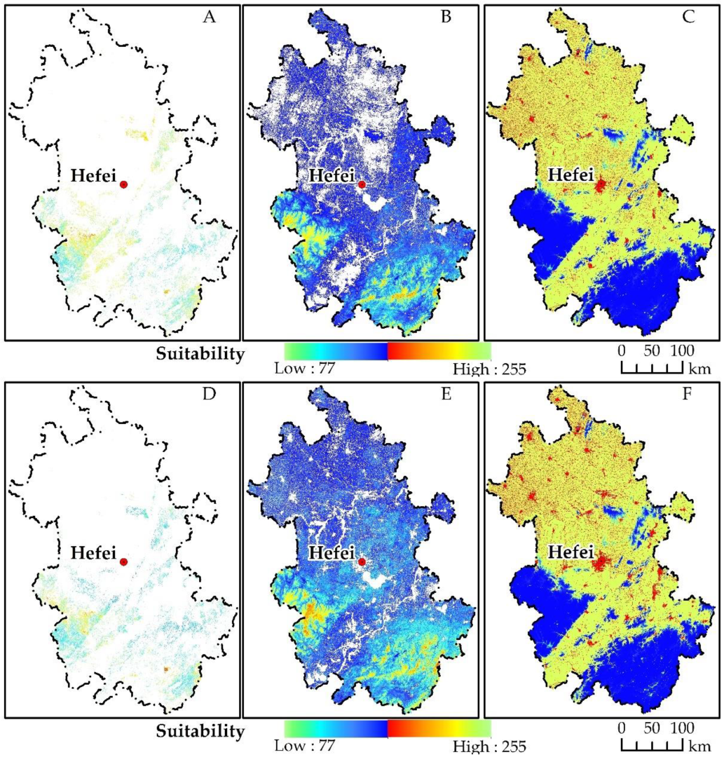
Suitability atlas is a spatial representation of the suitability of pine forest state transformation, that is, the comprehensive transformation rule of healthy pine forest, infected pine forest and non-pine forest, which refers to the degree of different types to which the region is suitable for development in a certain period of time in the future. When making the suitability atlas, it is necessary to consider two factors, limiting conditions and influencing conditions, in which the limiting factors specify whether pine forest state changes can occur in the region, and the influencing factors determine the change trend of suitable pine forest state, which is a continuous process.
According to the state of healthy pine forest, infected pine forest and non-pine forest, set the limiting conditions and influencing conditions, respectively, to make the suitability atlas, and then combine the suitability atlas to generate the model-readable suitability atlas (Figure 4). The multi-criteria evaluation (MCE) model is used to set the limiting factors and influencing factors of the suitability atlas (Table 2). The limiting factor of the infected pine forest (pine forest infected with PWD) is the construction land (from the artificial surface in the land use map), that is, PWD is unlikely to occur in this land type; the influencing factors are NDVI (average value in November and December of the current year and January and February of the next year), average wind speed, solar radiation intensity, population density, average relative humidity, average rainfall, maximum temperature, DEM, and distance from the road. The limiting factors of “healthy pine forest” and “non-pine forest” are all set with construction land. The influencing factors are NDVI and DEM, with weights of 0.6 and 0.4, respectively. The three pine forest states of healthy pine forest, infected pine forest and non-pine forest are transformed into each other according to the conditions set in Table 2 (i.e., limiting factors, influencing factors, functional relationships, and weights).
- (3)
- CA–Markov Prediction
CA–Markov prediction is based on the transition probability matrix, area matrix and suitability atlas of “pine forest state” of healthy pine forest, infected pine forest, and non-pine forest. Firstly, according to the transition probability matrix and area matrix of “pine forest state” in 2000 and 2010 and the 2010 suitability atlas, the occurrence of PWD in 2020 (Figure 5) is predicted, and the accuracy is verified according to the true value of the investigation of PWD in 2020, so as to evaluate whether the model can be used in this study and verify the rationality of the suitability atlas. After verifying that the model is usable and the suitability atlas is reasonable, based on the transition probability matrix and area matrix of “pine forest state” in 2010 and 2020 and the suitability atlas in 2020 as input data, the disaster occurrence in 2030 is predicted. In the prediction process, the CA–Markov model has two cycles, that is, the PWD in 2020 is predicted based on the relevant data in 2000 and 2010, and then the occurrence distribution map of PWD in 2030 is predicted based on the relevant data in 2010 and 2020, The setting of the number of cycles depends on the time interval between the base period year and the forecast year, which is usually a multiple of the study period interval. The research periods of this paper are 2000, 2010, 2020 and 2030, the time interval is 10, and the cycle number is set as 1, that is, the model is run at an interval of 10 years.
- (4)
- Simulation Accuracy Verification
The grid number error and error matrix (or “confusion matrix”) are used to verify the simulation accuracy.
where ri is the grid number error of class i, Sim is the actual number of pixels of class i, and Sin is the number of simulated pixels of class i.
The basic statistical indicators of the error matrix are: Overall accuracy (OA), User accuracy (UA), Product accuracy (PA), and Kappa coefficient (Kappa).
where r is the total number of columns in the error matrix (i.e., the total number of categories); is the number of pixels on the i row and i column of the error matrix (i.e., the number of analog types is the same as the real type, which is generally located on the diagonal of the error matrix); and are the sum of i row (analog type) and i column (real category), respectively; and N is the total number of samples. According to pertinent study [56], simulation accuracy can be evaluated according to Kappa. If Kappa is less than 0.4, it indicates that the simulation accuracy is too low, and if it is greater than 0.60, the simulation accuracy is high.
The result shows that the numerical accuracy error of disaster simulation grid is 4.81%, the OA is 93.19%, and the Kappa is 0.65. The comprehensive analysis shows that the CA–Markov model has high simulation accuracy for PWD in Anhui Province in 2020, and can be used to predict and simulate the occurrence of PWD in 2030. The prediction results are shown in Figure 6.
2.3.2. Directional Distribution
D. Welty Lefever proposed the directional distribution (standard deviation ellipse) algorithm, which expressed the spatial distribution trend of samples with parameters such as ellipse center and rotation angle in 1926. In this study, the standard deviation ellipse algorithm was used to reveal the spatial distribution characteristics of PWD infection spots. The formulas of standard deviation ellipse are:
where xi and yi are the spatial coordinates of each element; is the arithmetic mean center of the element; SDEx and SDEy are calculated variances of the ellipse; and n is the total number of elements. This study is the number of pine forest patch infected by PWD in each stage.
where θ refers to the clockwise rotation angle with the x-axis as the criterion and the true north (12 o’clock direction) as 0°, that is, the long axis direction of the standard deviation ellipse; and and are the differences between the average center and x-axis and y-axis coordinates of each patch.
The formula for calculating the standard deviation of x-axis and y-axis is as follows:
where and are the standard deviations of the X, Y axis.
where s is the confidence value; we can query the chi square probability table according to the number of elements. In spatial statistics, the direction of the ellipse is determined by the long and short semi-axes. The greater the oblateness of the ellipse, that is, the difference between the long and short semi-axes, indicating that the more obvious the directionality of the spatial distribution of the data, the higher the degree of aggregation and, on the contrary, the greater the degree of dispersion.
In this study, the direction distribution (standard deviation ellipse) tool in ArcGIS 10.3 software was used to analyze the direction trend of PWD infection spots in 2000, 2010, 2020 and 2030, that is, the major axis, minor axis, and oblateness of ellipse within 68% of the elements of PWD infection spots in each period were calculated according to the model.
2.3.3. Spatial Autocorrelation Analysis Method
Spatial autocorrelation analysis method refers to the correlation degree between a certain geographical phenomenon or an attribute value in a certain spatial region and the same phenomenon or attribute value in adjacent spatial regions [57]. Global spatial autocorrelation mainly studies the global spatial characteristics of attribute values, it is used to determine whether a phenomenon has spatial correlation. Moran’s I is usually used as the spatial autocorrelation index [58,59], as shown in Formula (15):
where is the overall Moran index, is the total number of spots of pine forest infected by PWD at each stage, is the spatial weight element value, and are the areas of infected spots of PWD, and is the average area of pine forest spots infected by PWD at each stage.
In this study, ArcGIS 10.3 software was used to analyze the global spatial autocorrelation of the infected spots of PWD, and to clarify the spatial distribution characteristics and spatial dependence of the infected spots of pine forest.
2.3.4. Topographic Analysis
(1) The influence of altitude on the distribution of pine trees is mainly reflected in the temperature and light conditions. In high altitude areas, the temperature is low and the soil is poor, which is not suitable for the growth of pine trees. Similarly, the relationship between PWD and altitude shows the same trend. When the altitude is less than 400 m, PWD occurs seriously; when the altitude is between 400–700 m, PWD occurs; when the altitude is more than 700 m, dead trees caused by PWD are rarely seen [60]. Therefore, combined with previous studies and field investigations, the altitude of pine forest distribution in the study area is divided into 15 intervals at an interval of 50 m.
(2) The impact of slope gradient on the distribution area of PWD is reflected in the aggregation and loss rate of soil nutrients, water content and other substances, which may affect the distribution or growth status of pine forests, due to inappropriate conditions, and then affect the spread of PWD. This study uses ArcGIS software to calculate the slope grid based on DEM data. Because the distribution gradient of pine forest in the study area is 0–50°, this study divides the slope of PWD in the study area into 5 intervals with an interval of 10°.
3. Results
Based on the spot survey of pine forest and PWD in Anhui Province in 2000, 2010 and 2020, the occurrence and spread of disasters in 2030 were predicted and simulated by using the CA–Markov model, and the spatial-temporal dynamic changes and distribution characteristics of disaster distribution in each period were analyzed.
3.1. Spatiotemporal Dynamic Changes in PWD
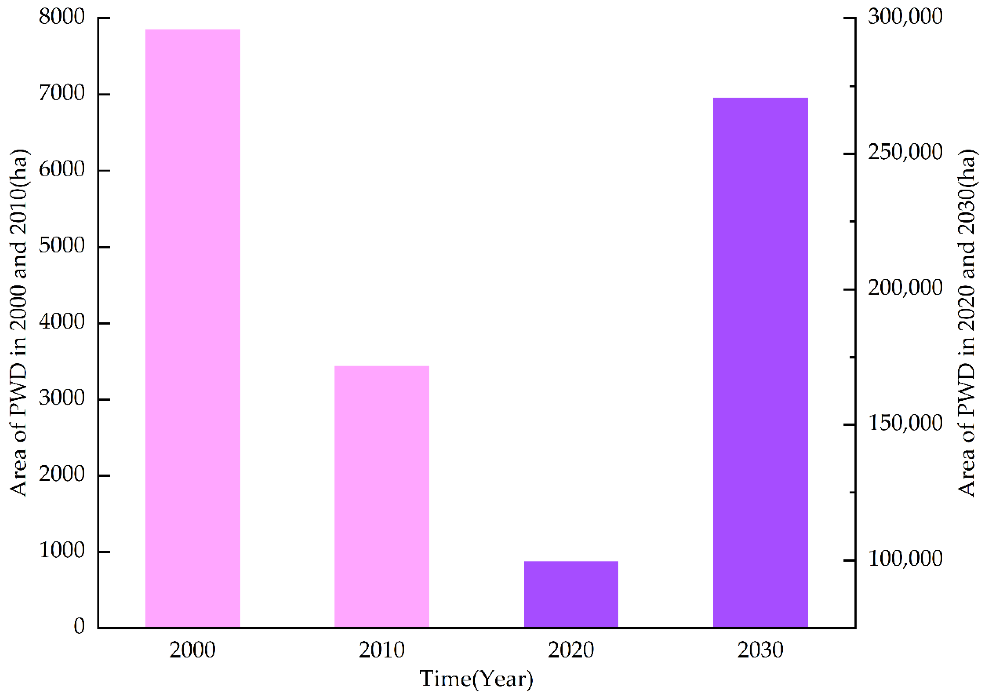
In the last 20 years, the occurrence area of PWD in Anhui Province has shown a trend of first decreasing and then increasing (Figure 5). After 2010, it witnessed a large outbreak trend. The disaster area increased rapidly, with an annual growth rate of 140%. By 2020, the disaster area had reached 29 times that of 2010. As the disaster base in 2020 is large, the annual growth rate of disaster (11%) in the next 10 years will slow down, but the growth trend is still rapid, and the occurrence area in 2030 will be 2.7 times that in 2020.
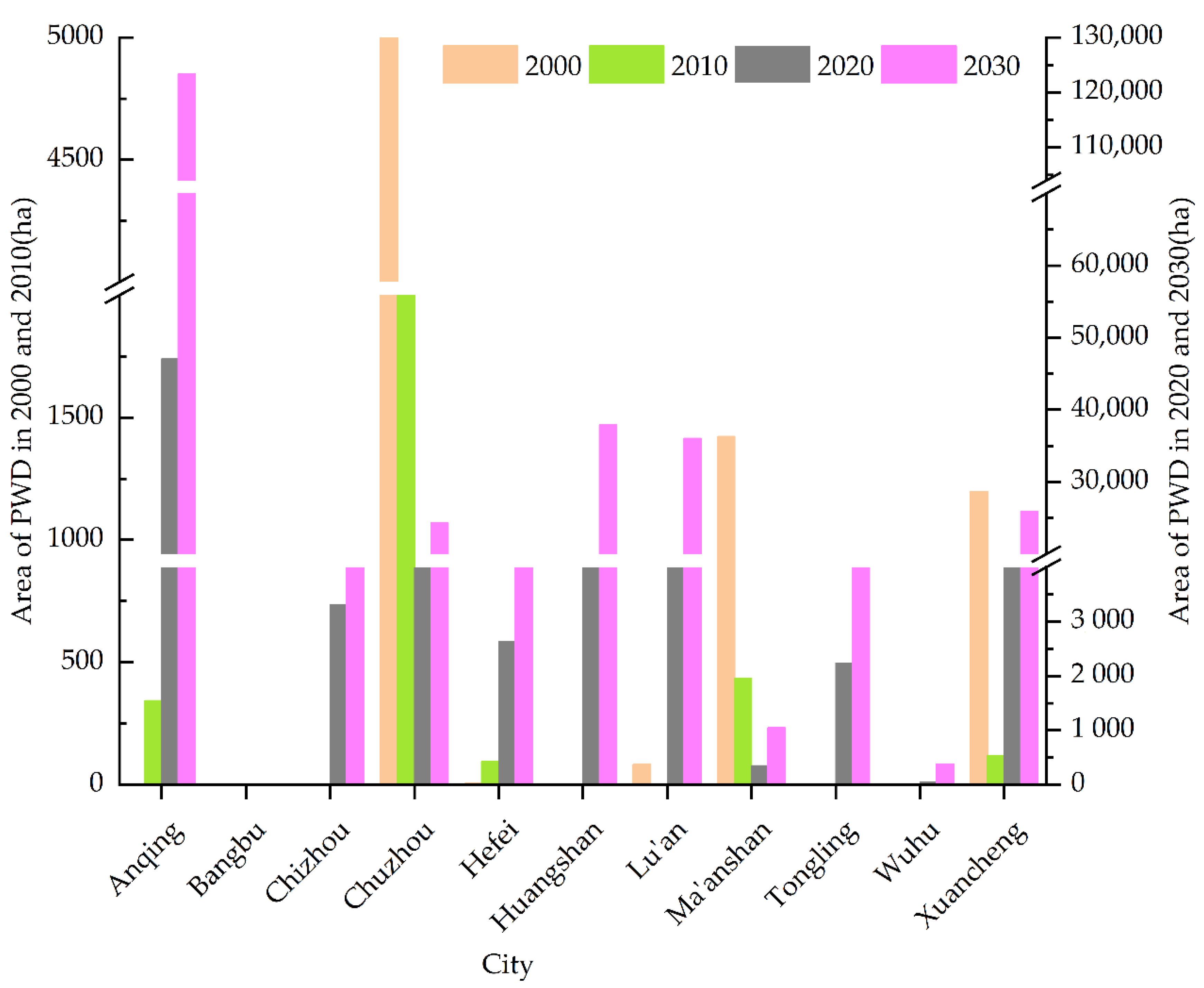
According to Figure 6 and Figure 7, the infected pine forests are widely distributed in the south of the study area, especially in the southwest, and there are many in Anqing, Lu’an, Chuzhou, and Xuancheng. The counties and districts with distribution of infected pine forests increased from 15, in 2000, to 47, in 2020 (see in Supplementary Table S1), showing an explosive growth. According to the forecast, it may reach 57 in 2030, covering almost all pine forest distribution counties (districts) in Anhui Province.
3.2. Spatial Autocorrelation Characteristics of PWD
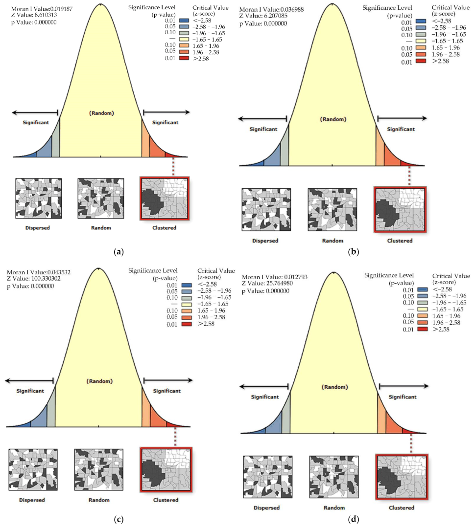
It can be seen from Figure 8 and Table 3 that the overall Moran’s I index in the distribution area of PWD in each year is greater than 0, and all of them pass the test of p value (≥1.96), indicating that the patches of PWD in each year presents a trend of concentrated distribution in space. In terms of time, Moran’s I and z-score first increased and then decreased, with the strongest in 2020. This shows that the occurrence areas of PWD in 2000, 2010 and 2020 are relatively concentrated, and there is a relatively clear source of occurrence, rather than a scattered disorderly dot-like occurrence, which is more conducive to post-disaster prevention and control. The further spread of the epidemic can be controlled by cutting down and destroying the infected trees. In 2030, the occurrence area of PWD still showed a trend of agglomeration. However, due to the large occurrence area and large diffusion range, the aggregation degree decreased compared with the first three stages.
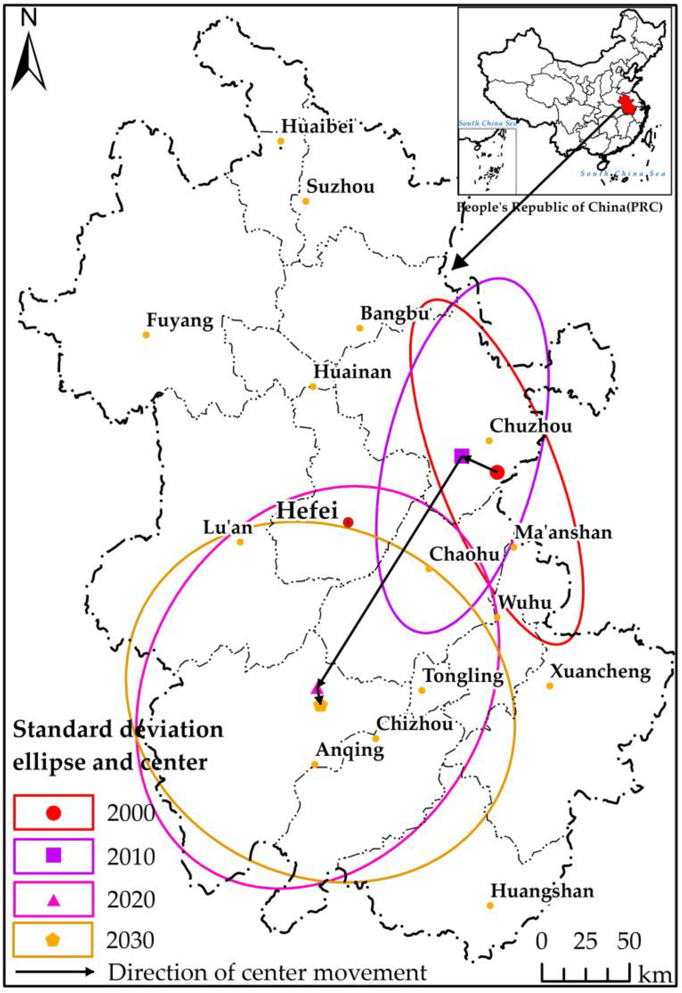
3.3. Characteristics of Directional Distribution and Center Movement of PWD
It can be seen from Figure 9 that the spatial distribution of the infected spots of PWD in 2000 and 2010 has significant directionality, which is northwest–southeast and northeast–southwest, respectively. With the continuous spread of the disease, the occurrence area and scope of PWD in 2020 and 2030 are larger than those in the previous two periods, and the spatial distribution directionality of the infected spots is gradually weakened. By 2030, the standard deviation ellipse is approximately circular.
As seen in Figure 9, in the past 20 years, the distribution center of PWD has a trend of moving southward. From 2000 to 2010, the disease occurrence center moved from inside Chuzhou to its northwest. From 2010 to 2020, the occurrence area changed significantly, that is, from Chuzhou to Anqing. By 2030, the occurrence area of PWD has further spread, and the focus of the disaster area is still in Anqing.
3.4. Distribution Characteristics of PWD According to Topographic Conditions
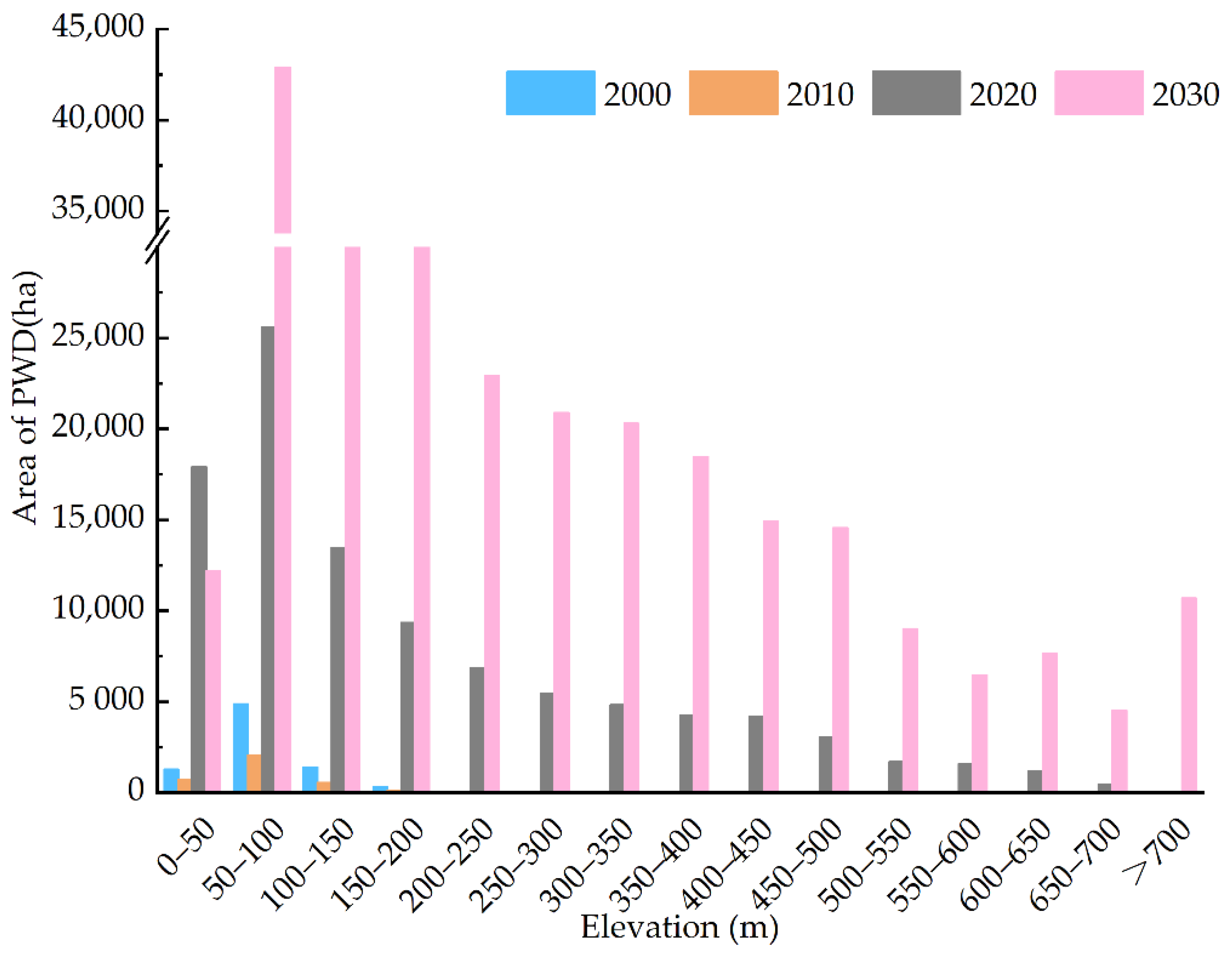
3.4.1. PWD Distribution along Elevation
According to Figure 10, by 2020, PWD occurs in the area below 700 m above sea level, and the frequency of PWD below 300 m is very high, with frequency values of 1.07% and approximately 0.00%, respectively. Therefore, 700 m can be regarded as the upper edge of the spatial distribution of PWD. Within the range of 0–700 m above sea level, the interval with the highest distribution frequency is 50–100 m, followed by 0–50 m and 100–150 m, with the frequencies of 29.30%, 17.89% and 13.86%, respectively. The three intervals account for 61.04% in total, indicating that nearly two-thirds of PWDs are distributed in the vertical space of 150 m, indicating that the spatial pattern of PWD and pine forest distribution is restricted by topographic factors such as altitude. Above 100 m, the distribution of PWD gradually decreases with the increase in altitude, especially in the area above 450 m, there is a sharp change trend. The prediction shows that the upper edge of the spatial distribution of PWD will break through 700 m in 2030. With the increase in altitude, the distribution area of the infected pine forest will gradually decrease.
Based on the data of the distribution of infected pine forests with altitude from 2000 to 2030, it is found that with the passage of time, the distribution altitude of PWD has gradually climbed, and the upward trend has become increasingly prominent.
3.4.2. PWD Distribution along Slope Gradient
According to Table 4, the proportion below 10° accounts for 53.16%, taking up the largest proportion; 10–20° accounts for 34.31%, 20–30° accounts for 11.37%, and 30–40° accounts for 1.09%. It can be seen that the slope condition in the region is more conducive to the growth and distribution of PWD, and it is not the main factor limiting the spread of PWD. With the passage of time, the average gradient of the distribution of infected pine forests has increased, especially after 2010, and the proportion of the distribution within 10° has decreased significantly. In 2030, the distribution of infected pine forests within 10° will account for less than 50%, indicating that with the influence of climate warming and other factors, the suitable range of PWD has expanded.
3.4.3. Distribution of PWD along Aspect
Table 5 shows that there are significant differences in the area distribution of infected pine forests in each aspect. Among them, the north slope accounts for 17.62%, with the highest proportion; the northwest slope accounts for 15.17%, holding the second highest; and the east slope and southeast slope account for 8.09% and 7.32%, respectively. It can be seen that the slope conditions in the region have a certain impact on the distribution of PWD. Sunshine in sunny slope is relatively abundant, which is more conducive to the spread of PWD. Compared with 2000, the proportion of infected pine forests in sunny slope increases in 2020. The forecast shows that the proportion of infected pine forests on sunny slope will further increase in 2030, and the proportion on shady slope will decrease significantly.
3.5. Relationship between the Occurrence Area and Road of PWD
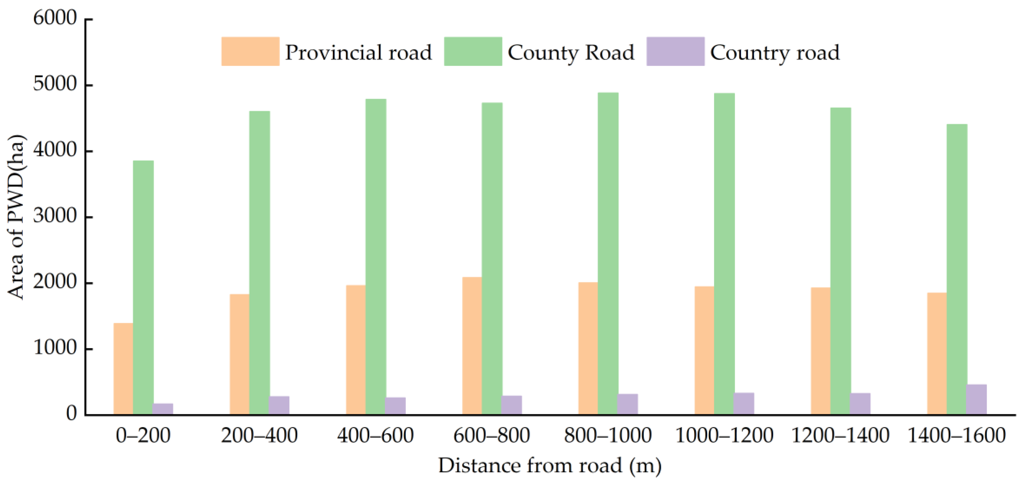
PWB (Monochamus alternatus) is the vector of PWD. During the transportation of wood or infected wood, PWB carrying the disease source of PWD will migrate to both sides of the transportation road [61], which will also cause PWD to spread along both sides of the road. By analyzing the buffer zone of the same grade roads of and superimposing the PWD map in each period, the infected area within different road distances (Figure 11 and Figure 12) is counted, and the Pearson correlation analysis method is used to quantitatively analyze the relationship between the occurrence area of PWD and road distance.
Figure 12 shows that the occurrence area of PWD on both sides of provincial and county roads is the largest within 800–1000 m away from the highway, and the infected area on both sides of township roads decreases gradually. While the infected area on both sides of township roads increases with the increase in distance, which may be related to the migration distance of PWB, and is similar to the research conclusion of Xiao [62]; that is, the migration distance of adults of PWB can generally reach 1.0–2.4 km.
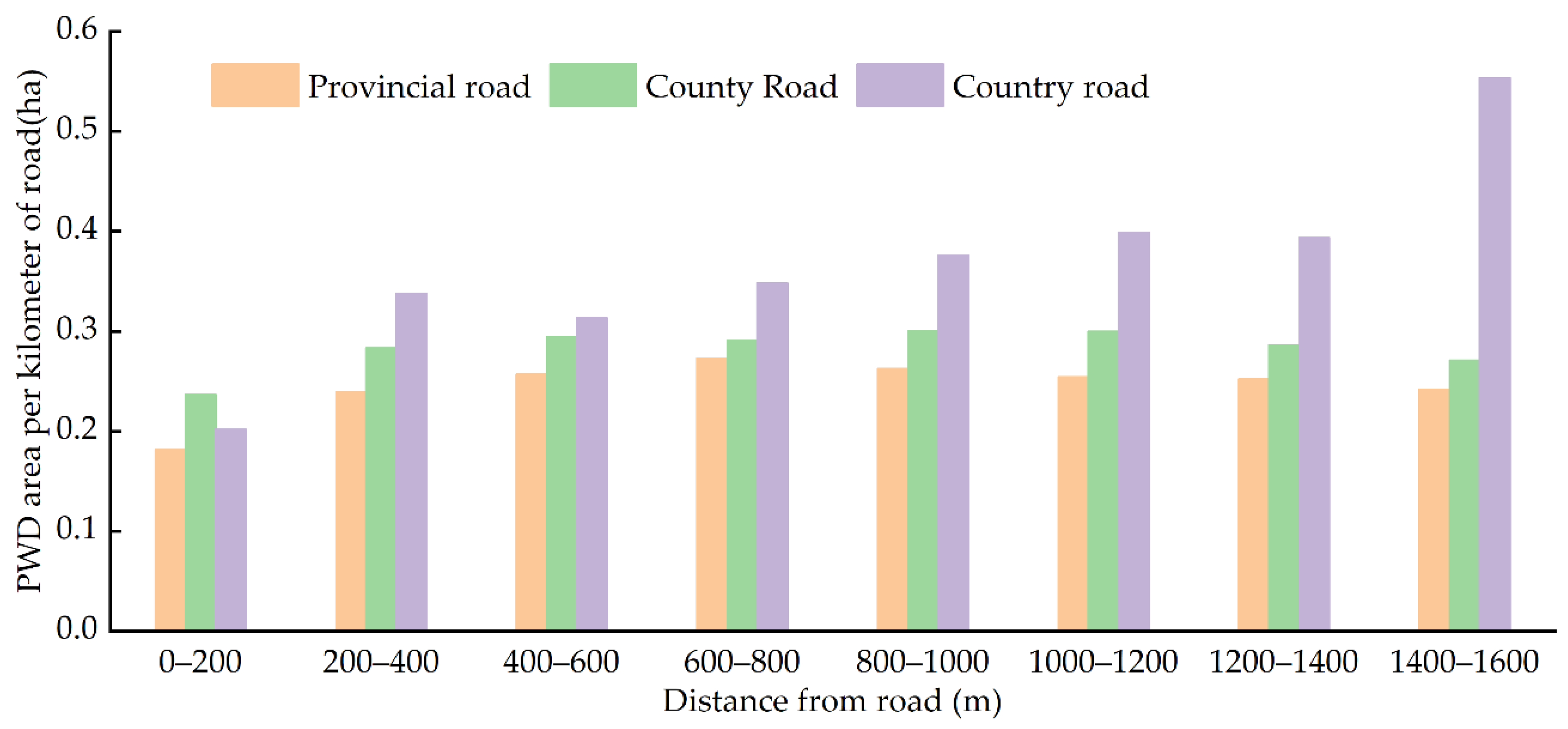
In order to compare the occurrence area of PWD in different types of highways, the total area in different distances and the total length of different grades of highways are used to obtain the occurrence area of PWD in unit distance of different types of highways. Figure 12 shows that the occurrence area of PWD in unit length of township roads is the largest, followed by county roads, and the smallest is provincial roads. The infected area of township roads increases with the increase in distance. In combination with Table 6, there is a significant correlation between the occurrence area of PWD and township roads, and the correlation is 0.896 and 0.950, respectively. This may be mainly because PWB may escape, or some infected branches and leaves may fall during the transportation of wood or infected wood on low-grade roads, and then the epidemic will spread along the way. With the increase in highway grade, the higher requirements on transport vehicles and goods appearance (such as the goods should be wrapped by tarpaulins) leads to the reduction in the number of escaping PWB, which may also be related to fewer vehicles transporting wood or infected wood on high-grade roads.
4. Discussion
4.1. Research Contributions
Based on the spot patch data of pine forest and PWD survey, this study creatively applied the CA–Markov model to forest disease prediction research, and realized the patch-level PWD occurrence prediction mapping in a province. The CA–Markov model combines all the advantages of the Cellular Automata model (CA) and the Markov model. It was first introduced into the field of geoscience by Tobler [63]. After continuous development, it is now widely used in land use/land cover (LULC) [64,65,66,67,68] and the study of urban landscape pattern evolution and prediction [69]. At present, there is a lack of research on the prediction of PWD, and the prediction of large-scale disease suitable areas [43] has been unable to meet the needs of precise and efficient prevention and control of multi-point frequently-occurring PWD. The simulation ability of the CA–Markov model to spatiotemporal dynamic change can not only meet the needs of LULC change simulation research, but also apply to the prediction of affected areas of land cover change caused by pests. In this study, the CA–Markov model is applied to the prediction of PWD for the first time, and the large-scale (provincial scale) fine-grained (map spot level) PWD occurrence prediction mapping is realized, with an accuracy of 93.19%. Our prediction result is that it is strictly limited to the pine forest coverage area, which is of great help to guide the PWD disaster prevention and control in Anhui Province in the next 10 years. This method is not only used in this study area, but can also be applied to PWD prediction in other areas.
4.2. Limitations and Prospects
It is worth noting that this paper has limitations for further research. Firstly, it is difficult to obtain historical data of pine forest and PWD distribution based on patches. Not all regions can obtain such detailed data, which limits the wide application of this method. Secondly, the spatial resolution of some data used in this paper is not high (for example, the spatial resolution of meteorological data is 5000 m), which may lead to the neglect of some spatial heterogeneity features in the prediction process of PWD, and may ultimately affect the prediction accuracy. However, this effect may only occur in areas with significant elevation changes. As we all know, elevation can redistribute temperature and precipitation.
With the continuous enrichment of remote sensing big data resources and the improvement of temporal and spatial resolution, the patch-based pine forest and PWD distribution data provided by the forestry department in this paper may be replaced by the big data remote sensing interpretation results, which has great potential for the wide application of PWD prediction based on the CA–Markov model.
4.3. Countermeasures and Suggestions
PWD is known as the “cancer” of pine trees [70]. Once pine trees are infected, they will perish. We hope to control the spread of PWD and reduce its losses to pine forests and ecosystems by strengthening the timely monitoring, early warning, and decisive management of PWD. According to the findings in Section 3.5, we suggest that during the removal and transportation of PWD infected trees, all the litter of the trees should be completely cleaned to avoid the risk of PWD transmission caused by the fall of pine branches infected with PWD during the transportation.
5. Conclusions
In this study, taking Anhui Province as the study area, the CA–Markov model was used to predict and calculate the occurrence area of PWD in Anhui Province in 2030. Spatial autocorrelation analysis, standard deviation ellipse (direction) analysis and other spatial analysis methods are used to analyze the occurrence data of PWD in 2000, 2010, 2020 and 2030, and to clarify the spatio-temporal dynamic changes and distribution laws of PWD in Anhui Province. (1) The CA–Markov model can be used to predict the disaster of PWD, and can accurately predict the location and area of the disease in the next decade; (2) the infected area of PWD in Anhui province increased rapidly, with the characteristics of clustering distribution, and the disease center spread from northeast to southwest; (3) the topography has certain restrictions on the spatial distribution of PWD. In the next 10 years, the infected areas will break through the traditional suitable areas and spread to high altitude, high slope, and sunny slope areas.
Supplementary Materials
The following supporting information can be downloaded at: https://www.mdpi.com/article/10.3390/f13101736/s1, Supplementary Table S1: Area of pine wood nematode disease by county and city in Anhui Province, by year. Figure S1: Workflow of PWD prediction based on CA–Markov model.
Author Contributions
Conceptualization, D.L. and X.Z.; methodology, D.L. and X.Z.; formal analysis, D.L. and X.Z.; investigation, D.L. and X.Z.; resources, D.L. and X.Z.; data curation, D.L.; writing—original draft preparation, D.L.; writing—review and editing, D.L.; visualization, D.L.; supervision, D.L. and X.Z.; project administration, X.Z.; funding acquisition, X.Z. All authors have read and agreed to the published version of the manuscript.
Funding
This research was funded by the National Natural Science Foundation of China (Fund No. 31870534).
Data Availability Statement
Data are available from the authors upon reasonable request as the data need further use.
Acknowledgments
We appreciate the critical and constructive comments from three anonymous reviewers and thank all editors that participated in the revision process.
Conflicts of Interest
The authors declare no conflict of interest.
References
- Olsson, P.; Heliasz, M.; Jin, H.; Eklundh, L. Mapping the reduction in gross primary productivity in subarctic birch forests due to insect outbreaks. Biogeosciences 2017, 14, 1703–1719. [Google Scholar] [CrossRef] [Green Version]
- Bergdahl, D.R. Impact of pinewood nematode in North America: Present and future. J. Nematol. 1988, 20, 260–265. [Google Scholar] [PubMed]
- Li, Y.; Zhang, X. Analysis on the trend of invasion and expansion of Bursaphelenchus xylophilus. For. Pest Dis. 2018, 37, 1–4. [Google Scholar]
- State Forestry and Grassland Administration. 2022 Announcement of Pine Wood Nematode Epidemic Area. Available online: http://www.gzhs.gov.cn/zfbm/hsxlyj_5721086/zcwj_5721053/202205/t20220511_73990365.html (accessed on 29 July 2022).
- Gent, D.H.; Schwartz, H.F. Validation of potato early blight disease forecast models for Colorado using various sources of meteorological data. Plant Dis. 2003, 87, 78–84. [Google Scholar] [CrossRef] [PubMed]
- Roubal, C.; Regis, S.; Nicot, P.C. Field models for the prediction of leaf infection and latent period of Fusicladium oleagineum on olive based on rain, temperature and relative humidity. Plant Pathol. 2013, 62, 657–666. [Google Scholar] [CrossRef]
- Kumar, A.; Agrawal, R.; Chattopadhyay, C. Weather based forecast models for diseases in mustard crop. Mausam 2013, 64, 663–670. [Google Scholar] [CrossRef]
- Valdez-Torres, J.B.; Soto-Landeros, F.; Osuna-Enciso, T.; Baez-Sanudo, M.A. Phenological prediction models for white corn (Zea mays L.) and fall armyworm (Spodoptera frugiperda J.E. Smith). Agrociencia 2012, 46, 399–410. [Google Scholar]
- Schwartz, M.W. Potential effects of global climate change on the biodiversity of plants. For. Chron. 1992, 68, 462–471. [Google Scholar] [CrossRef]
- Laderach, P.; Ramirez-Villegas, J.; Navarro-Racines, C.; Zelaya, C.; Martinez-Valle, A.; Jarvis, A. Climate change adaptation of coffee production in space and time. Clim. Chang. 2017, 141, 47–62. [Google Scholar] [CrossRef] [Green Version]
- Dukes, J.S.; Pontius, J.; Orwig, D.; Garnas, J.R.; Rodgers, V.L.; Brazee, N.; Cooke, B.; Theoharides, K.A.; Stange, E.E.; Harrington, R.; et al. Responses of insect pests, pathogens, and invasive plant species to climate change in the forests of northeastern North America: What can we predict? Can. J. For. Res. 2009, 39, 231–248. [Google Scholar] [CrossRef]
- Brown, N.; Vanguelova, E.; Parnell, S.; Broadmeadow, S.; Denman, S. Predisposition of forests to biotic disturbance: Predicting the distribution of Acute Oak Decline using environmental factors. For. Ecol. Manag. 2018, 407, 145–154. [Google Scholar] [CrossRef]
- Giliba, R.A.; Mpinga, I.H.; Ndimuligo, S.A.; Mpanda, M.M. Changing climate patterns risk the spread of Varroa destructor infestation of African honey bees in Tanzania. Ecol. Process. 2020, 9, 48. [Google Scholar] [CrossRef]
- Guru-Pirasanna-Pandi, L.G.; Choudhary, J.S.; Chemura, A.; Basana-Gowda, G.; Annamalai, M.; Patil, N.; Adak, T.; Rath, P.C. Predicting the brown planthopper, Nilaparvata lugens (Stal) (Hemiptera: Delphacidae) potential distribution under climatic change scenarios in India. Curr. Sci. India 2021, 121, 1600–1609. [Google Scholar] [CrossRef]
- Bosso, L.; Di Febbraro, M.; Cristinzio, G.; Zoina, A.; Russo, D. Shedding light on the effects of climate change on the potential distribution of Xylella fastidiosa in the Mediterranean basin. Biol. Invasions 2016, 18, 1759–1768. [Google Scholar] [CrossRef]
- Bosso, L.; Russo, D.; Di Febbraro, M.; Cristinzio, G.; Zoina, A. Potential distribution of Xylella fastidiosa in Italy: A maximum entropy model. Phytopathol. Mediterr. 2016, 55, 62–72. [Google Scholar] [CrossRef]
- Poutsma, J.; Loomans, A.; Aukema, B.; Heijerman, T. Predicting the potential geographical distribution of the harlequin ladybird, Harmonia axyridis, using the CLIMEX model. BioControl 2008, 53, 103–125. [Google Scholar] [CrossRef]
- Phillips, S.J.; Anderson, R.P.; Schapire, R.E. Maximum entropy modeling of species geographic distributions. Ecol. Model. 2006, 190, 231–259. [Google Scholar] [CrossRef] [Green Version]
- Peterson, A.T.; Papes, M.; Eaton, M. Transferability and model evaluation in ecological niche modeling: A comparison of GARP and Maxent. Ecography 2007, 30, 550–560. [Google Scholar] [CrossRef]
- Beaumont, L.J.; Hughes, L.; Poulsen, M. Predicting species distributions: Use of climatic parameters in BIOCLIM and its impact on predictions of species’ current and future distributions. Ecol. Model. 2005, 186, 250–269. [Google Scholar] [CrossRef]
- Kelly, M.; Meentemeyer, R.K. Landscape dynamics of the spread of sudden oak death. Photogramm. Eng. Remote Sens. 2002, 68, 1001–1010. [Google Scholar]
- Volpi, I.; Guidotti, D.; Mammini, M.; Marchi, S. Predicting symptoms of downy mildew, powdery mildew, and gray mold diseases of grapevine through machine learning. Ital. J. Agrometeorol. 2021, 2, 57–69. [Google Scholar] [CrossRef]
- BenDor, T.K.; Metcalf, S.S.; Fontenot, L.E.; Sangunett, B.; Hannon, B. Modeling the spread of the emerald ash borer. Ecol. Model. 2006, 197, 221–236. [Google Scholar] [CrossRef]
- Howell, B.E.; Burns, K.S.; Kearns, H.S. Biological Evaluation of a Model for Predicting Presence of White Pine Blister Rust in Colorado Based on Climatic Variables and Susceptible White Pine Species Distribution: USDA Forest Service, Rocky Mountain Region, Renewable Resources. 2006. Available online: http://www.fs.usda.gov/Internet/FSE_DOCUMENTS/fsbdev3_039457.pdf (accessed on 20 September 2022).
- Wang, S.H.; Dai, J.G.; Zhao, Q.Z.; Cui, M.N. Application of grey systems in predicting the degree of cotton spider mite infestations. Grey Syst. Theory Appl. 2017, 7, 353–364. [Google Scholar] [CrossRef]
- Aparecido, L.; Rolim, G.D.; De Moraes, J.; Costa, C.; de Souza, P.S. Machine learning algorithms for forecasting the incidence of Coffea arabica pests and diseases. Int. J. Biometeorol. 2020, 64, 671–688. [Google Scholar] [CrossRef]
- Fabre, F.; Pierre, J.S.; Dedryver, C.A.; Plantegenest, M. Barley yellow dwarf disease risk assessment based on Bayesian modelling of aphid population dynamics. Ecol. Model. 2006, 193, 457–466. [Google Scholar] [CrossRef]
- Hanks, E.M.; Hooten, M.B.; Baker, F.A. Reconciling multiple data sources to improve accuracy of large-scale prediction of forest disease incidence. Ecol. Appl. 2011, 21, 1173–1188. [Google Scholar] [CrossRef] [PubMed]
- Iordache, M.; Mantas, V.; Baltazar, E.; Pauly, K.; Lewyckyj, N. A machine learning approach to detecting pine wilt disease using airborne spectral imagery. Remote Sens. 2020, 12, 2280. [Google Scholar] [CrossRef]
- Wu, W.; Zhang, Z.; Zheng, L.; Han, C.; Wang, X.; Xu, J.; Wang, X. Research Progress on the Early Monitoring of Pine Wilt Disease Using Hyperspectral Techniques. Sensors 2020, 20, 3729. [Google Scholar] [CrossRef]
- Lee, D.; Choi, W.I.; Nam, Y.; Park, Y. Predicting potential occurrence of pine wilt disease based on environmental factors in South Korea using machine learning algorithms. Ecol. Inform. 2021, 64, 101378. [Google Scholar] [CrossRef]
- Han, Y.; Wang, Y.; Xiang, Y.; Ye, J. Prediction of potential distribution of Bursaphelenchus xylophilus in China based on Maxent ecological niche model. J. Nanjing For. Univ. (Nat. Sci. Ed.) 2015, 39, 6–10. [Google Scholar] [CrossRef]
- Li, M.Y.; Liu, M.L.; Liu, M.; Ju, Y.W. Prediction of Pine Wilt Disease in Jiangsu Province Based on Web Dataset and GIS. In Web Information Systems and Mining; Springer: Berlin/Heidelberg, Germany, 2010; Volume 6318, pp. 146–153. [Google Scholar]
- Ju, Y.; Li, M.; Wu, W. Predictive Methods of Pine Wilt Disease in Jiangsu Province. Sci. Silvae Sin. 2010, 46, 91–96. [Google Scholar]
- He, S.; Wen, J.; Luo, Y.; Zong, S.; Zhao, Y.; Han, J. The predicted geographical distribution of Bursaphelenchus xylophilus in China under climate warming. Chin. J. Appl. Entomol. 2012, 49, 236–243. [Google Scholar]
- Zhao, J.; Han, X.; Shi, J. Potential distribution of Bursaphelenchus xylophilus in China due to adaptation cold conditions. J. Biosaf. 2017, 26, 191–198. [Google Scholar]
- Gruffudd, H.R.; Jenkins, T.A.R.; Evans, H.F. Using an evapo-transpiration model (ETpN) to predict the risk and expression of symptoms of pine wilt disease (PWD) across Europe. Biol. Invasions 2016, 18, 2823–2840. [Google Scholar] [CrossRef]
- An, H.; Lee, S.; Cho, S.J. The Effects of Climate Change on Pine Wilt Disease in South Korea: Challenges and Prospects. Forests 2019, 10, 486. [Google Scholar] [CrossRef] [Green Version]
- Hirata, A.; Nakamura, K.; Nakao, K.; Kominami, Y.; Tanaka, N.; Ohashi, H.; Takano, K.T.; Takeuchi, W.; Matsui, T. Potential distribution of pine wilt disease under future climate change scenarios. PLoS ONE 2017, 12, e0182837. [Google Scholar] [CrossRef]
- de la Fuente, B.; Saura, S.; Beck, P. Predicting the spread of an invasive tree pest: The pine wood nematode in Southern Europe. J. Appl. Ecol. 2018, 55, 2374–2385. [Google Scholar] [CrossRef]
- de la Fuente, B.; Saura, S. Long-Term Projections of the Natural Expansion of the Pine Wood Nematode in the Iberian Peninsula. Forests 2021, 12, 849. [Google Scholar] [CrossRef]
- Hao, Z.; Fang, G.; Huang, W.; Ye, H.; Zhang, B.; Li, X. Risk Prediction and Variable Analysis of Pine Wilt Disease by a Maximum Entropy Model. Forests 2022, 13, 342. [Google Scholar] [CrossRef]
- Tang, X.; Yuan, Y.; Li, X.; Zhang, J. Maximum Entropy Modeling to Predict the Impact of Climate Change on Pine Wilt Disease in China. Front. Plant Sci. 2021, 12, 652500. [Google Scholar] [CrossRef]
- Nguyen, T.V.; Park, Y.; Jeoung, C.; Choi, W.; Kim, Y.; Jung, I.; Shigesada, N.; Kawasaki, K.; Takasu, F.; Chon, T. Spatially explicit model applied to pine wilt disease dispersal based on host plant infestation. Ecol. Model. 2017, 353, 54–62. [Google Scholar] [CrossRef]
- Takasu, F. Individual-based modeling of the spread of pine wilt disease: Vector beetle dispersal and the Allee effect. Popul. Ecol. 2009, 51, 399–409. [Google Scholar] [CrossRef]
- Robinet, C.; Van Opstal, N.; Baker, R.; Roques, A. Applying a spread model to identify the entry points from which the pine wood nematode, the vector of pine wilt disease, would spread most rapidly across Europe. Biol. Invasions 2011, 13, 2981–2995. [Google Scholar] [CrossRef] [Green Version]
- Yoshimura, A.; Kawasaki, K.; Takasu, F.; Togashi, K.; Futai, K.; Shigesada, N. Modeling the spread of pine wilt disease caused by nematodes with pine sawyers as vector. Ecology 1999, 80, 1691–1702. [Google Scholar] [CrossRef]
- Choi, W.I.; Song, H.J.; Kim, D.S.; Lee, D.; Lee, C.; Nam, Y.; Kim, J.; Park, Y. Dispersal Patterns of Pine Wilt Disease in the Early Stage of Its Invasion in South Korea. Forests 2017, 8, 411. [Google Scholar] [CrossRef] [Green Version]
- Aslam, A.; Ozair, M.; Hussain, T.; Awan, A.U.; Tasneem, F.; Shah, N.A. Transmission and epidemiological trends of pine wilt disease: Findings from sensitivity to optimality. Results Phys. 2021, 26, 104443. [Google Scholar] [CrossRef]
- Shi, X.; Song, G. Analysis of the Mathematical Model for the Spread of Pine Wilt Disease. J. Appl. Math. 2013, 2013, 184054. [Google Scholar] [CrossRef] [Green Version]
- Dimitrijevic, D.D.; Bacic, J. Mathematical analysis of dynamic spread of Pine Wilt disease. Commun. Agric. Appl. Biol. Sci. 2013, 78, 389–399. [Google Scholar]
- Kobayashi, F.; Yamane, A.; Ikeda, T. The Japanese pine sawyer beetle as the vector of pine wilt disease. Annu. Rev. Entomol. 1984, 29, 115–135. [Google Scholar] [CrossRef]
- Deng, R.; Guo, F. Occurrence regularity and control strategy of pine wood nematode in Shangyou County. J. Green Sci. Technol. 2019, 21, 204–205. [Google Scholar]
- Jing, Y.; Zhang, F.; Zhang, Y. Change and prediction of the land use /cover in Ebinur Lake Wetland Nature Reserve based on CA-Markov model. Chin. J. Appl. Ecol. 2016, 27, 3649–3658. [Google Scholar] [CrossRef]
- Zhou, C.; Ou, Y.; Ma, T.; Tan, B. Theoretical Perspectives of CA-based Geographical System Modeling. Prog. Geogr. 2009, 28, 833–838. [Google Scholar]
- Xin, F.; Wang, X.; Yang, Y.J. Deriving suitability factors for CA-Markov land use simulation model based on local historical data. J. Environ. Manag. 2017, 206, 10–19. [Google Scholar]
- Jossart, J.; Theuerkauf, S.J.; Wickliffe, L.C.; Morris, J.A., Jr. Applications of Spatial Autocorrelation Analyses for Marine Aquaculture Siting. Front. Mar. Sci. 2020, 6, 806. [Google Scholar] [CrossRef]
- Rangel, T.; Diniz-Filho, J.; Bini, L.M.; Rangel, T.; Diniz-Filho, J.A.F.; Bini, L.M. Towards an integrated computational tool for spatial analysis in macroecology and biogeography. Glob. Ecol. Biogeogr. 2006, 15, 321–327. [Google Scholar] [CrossRef]
- Hao, Z.; Huang, J.; Zhou, Y.; Fang, G. Spatiotemporal Pattern of Pine Wilt Disease in the Yangtze River Basin. Forests 2021, 12, 731. [Google Scholar] [CrossRef]
- Zhang, X. Major Biological Disaster of Forest in China; China Forestry Press: Beijing, China, 2003. [Google Scholar]
- Li, Y. Landscape Patterns on Influence of Population Density and Genetic diversity of Monochamus alternatus Hope (Coleoptera: Cerambycidae). Master’s Thesis, Fujian Agriculture and Forestry University, Fuzhou, China, 2020. [Google Scholar] [CrossRef]
- Xiao, G. Forest Insects in China, 2nd ed.; China Forestry Press: Beijing, China, 1992. [Google Scholar]
- Tobler, W.R. A computer movie simulating urban growth in the Detroit region. Econ. Geogr. 1970, 46, 234–240. [Google Scholar] [CrossRef]
- Zhang, X.; Zhou, J.; Li, M. Analysis on spatial and temporal changes of regional habitat quality based on the spatial pattern reconstruction of land use. Acta Geogr. Sin. 2020, 75, 160–178. [Google Scholar]
- Zhao, J.; Zhang, H.; Qiao, Z.; Zhang, Z.; Hou, G. Dynamic simulation of land cover change in Xianghai wetland based on CA-Markov model. J. Nat. Resour. 2009, 24, 2178–2186. [Google Scholar]
- Cui, L.; Zhao, Y.H.; Liu, J.C.; Wang, H.Y.; Han, L.; Li, J.; Sun, Z.H. Vegetation Coverage Prediction for the Qinling Mountains Using the CA-Markov Model. ISPRS Int. J. Geo-Inf. 2021, 10, 679. [Google Scholar] [CrossRef]
- Rimal, B.; Zhang, L.F.; Keshtkar, H.; Wang, N.; Lin, Y. Monitoring and Modeling of Spatiotemporal Urban Expansion and Land-Use/Land-Cover Change Using Integrated Markov Chain Cellular Automata Model. ISPRS Int. J. Geo-Inf. 2017, 6, 288. [Google Scholar] [CrossRef]
- Mondal, M.S.; Sharma, N.; Kappas, M.; Garg, P.K. Modeling of spatio-temporal dynamics of land use and land cover in a part of Brahmaputra River basin using Geoinformatic techniques. Geocarto Int. 2013, 28, 632–656. [Google Scholar] [CrossRef]
- Luo, Z.; Hu, X.; Wei, B.; Cao, P.; Cao, S.; Du, X. Urban Landscape Pattern Evolution and Prediction Based on Multi-Criteria CA-Markov Model:Take Shanghang County as an Example. Econ. Geogr. 2020, 40, 58–66. [Google Scholar] [CrossRef]
- Lu, X.; Huang, J.; Li, X.; Fang, G.; Liu, D. The interaction of environmental factors increases the risk of spatiotemporal transmission of pine wilt disease. Ecol. Indic. 2021, 133, 108394. [Google Scholar] [CrossRef]
Figure 1.
Location of the study area.

Figure 2.
Map of pine forest and PWD.
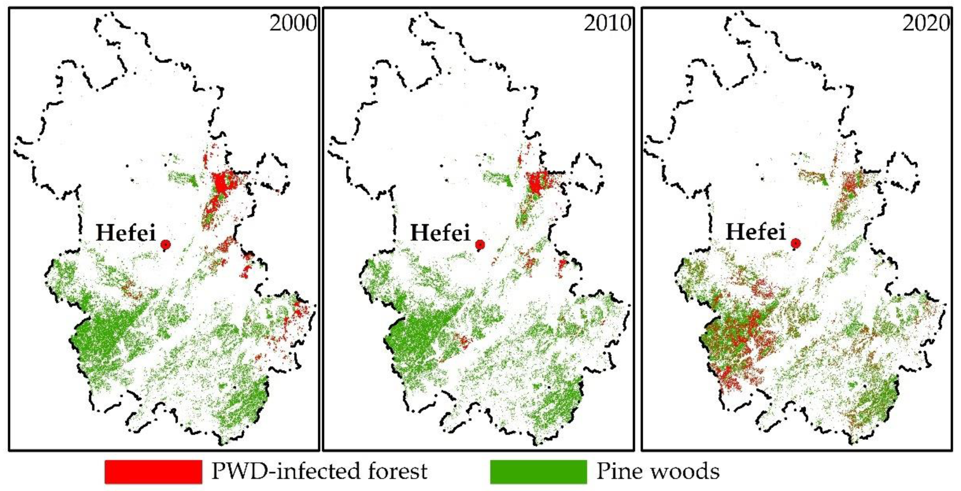
Figure 3.
The technical framework of the proposed method.

Figure 4.
Pine state suitability atlas (A,D) are non-healthy pine forests in 2010 and 2020, respectively; (B,E) are health pine forests in 2010 and 2020, respectively; (C,F) are non-pine forest in 2010 and 2020, respectively.
Figure 4.
Pine state suitability atlas (A,D) are non-healthy pine forests in 2010 and 2020, respectively; (B,E) are health pine forests in 2010 and 2020, respectively; (C,F) are non-pine forest in 2010 and 2020, respectively.

Figure 5.
The annual occurrence area of PWD in Anhui Province.

Figure 6.
Occurrence area of PWD in different periods in cities of Anhui Province.

Figure 7.
Spatial distribution of PWD in Anhui Province (superposition of 4 periods).

Figure 8.
Spatial autocorrelation analysis results of PWD distribution in different years ((a–d) are 2000, 2010, 2020 and 2030, respectively).
Figure 8.
Spatial autocorrelation analysis results of PWD distribution in different years ((a–d) are 2000, 2010, 2020 and 2030, respectively).

Figure 9.
Map of directional distribution and center movement of PWD in different periods.

Figure 10.
Statistics of vertical distribution of PWD along altitude.

Figure 11.
Relationship between occurrence area of PWD and road distance in Anhui province in 2020.

Figure 12.
Relationship between occurrence area of PWD per unit length of road and distance of road in 2020.
Figure 12.
Relationship between occurrence area of PWD per unit length of road and distance of road in 2020.


Table 1.
Markov transition probability matrix.
| Time | 2010 | Time | 2020 | ||||||
|---|---|---|---|---|---|---|---|---|---|
| States of Pine Forest | Healthy Pine Forest | Infected Pine Forest | Non-Pine Forest | States of Pine Forest | Healthy Pine Forest | Infected Pine Forest | Non-Pine Forest | ||
| 2000 | healthy pine forest | 0.8472 | 0.1528 | 0 | 2010 | healthy pine forest | 0.7682 | 0.2318 | 0 |
| infected pine forest | 0 | 0 | 1 | infected pine forest | 0 | 0 | 1 | ||
| non-pine forest | 0.065 | 0.0125 | 0.9225 | non-pine forest | 0.0439 | 0.0202 | 0.9359 | ||
Table 2.
The elements and weights table of PWD suitability atlas.
| Limiting Factors | Influencing Factors | Functional Relationships | Weights |
|---|---|---|---|
| Building up | NDVI | Diminishing—J Shape | 0.205 |
| / | Average wind speed | Diminishing—Sigmoidal | 0.203 |
| / | Solar radiation intensity | Diminishing—Sigmoidal | 0.104 |
| / | Population density | Diminishing—J Shape | 0.073 |
| / | Average relative humidity | Diminishing—J Shape | 0.052 |
| / | Average rainfall | Diminishing—Sigmoidal | 0.034 |
| / | Maximum temperature | Diminishing—Sigmoidal | 0.032 |
| / | DEM | Diminishing—Sigmoidal | 0.007 |
| / | Distance from the road | Diminishing—Sigmoidal | 0.29 |
Table 3.
Spatial autocorrelation Moran’s I report of PWD distribution in each year.
| Years | Moran’s I | Z-Score | p Value |
|---|---|---|---|
| 2000 | 0.019187 | 8.610313 | 0.000000 |
| 2010 | 0.036988 | 6.207085 | 0.000000 |
| 2020 | 0.043532 | 100.330302 | 0.000000 |
| 2030 | 0.012793 | 25.764980 | 0.000000 |
Table 4.
Distribution area of PWD along slope gradient in different years.
| Year | Distribution Area of PWD on Different Grade Slope/ha | |||||
|---|---|---|---|---|---|---|
| 1 | 2 | 3 | 4 | 5 | Total | |
| 2000 | 7066 | 665 | 126 | 7857 | ||
| 2010 | 3190 | 206 | 43 | 3440 | ||
| 2020 | 64,695 | 26,884 | 7385 | 640 | 0.41 | 99,605 |
| 2030 | 127,888 | 103,165 | 35,824 | 3509 | 245 | 270,632 |
| Total | 202,839 | 130,920 | 43,378 | 4149 | 245 | 381,532 |
Table 5.
Distribution area of PWD along aspect in each year in the study area.
| Year | Distribution Area of PWD on Different Grade Aspect/ha | ||||||||
|---|---|---|---|---|---|---|---|---|---|
| North | Northeast | East | Southeast | South | Southwest | West | Northwest | Total | |
| 2000 | 1229 | 864 | 618 | 481 | 841 | 1094 | 1500 | 1231 | 7857 |
| 2010 | 595 | 427 | 211 | 285 | 344 | 456 | 526 | 597 | 3440 |
| 2020 | 17,718 | 12,083 | 8145 | 7349 | 10,879 | 13,677 | 14,761 | 14,993 | 99,605 |
| 2030 | 32,116 | 22,449 | 16,676 | 28,875 | 40,058 | 42,158 | 45,328 | 42,972 | 270,632 |
| Total | 51,658 | 35,822 | 25,649 | 36,990 | 52,122 | 57,384 | 62,115 | 59,792 | 381,533 |
Table 6.
Correlation analysis between PWD area and road distance.
| Road Type | 2020 Correlation | 2030 Correlation |
|---|---|---|
| Provincial road | 0.491 | 0.626 |
| County Road | 0.392 | 0.270 |
| Country road | 0.896 ** | 0.950 ** |
** indicates a significant correlation at the 0.01 level (two-tailed).
Publisher’s Note: MDPI stays neutral with regard to jurisdictional claims in published maps and institutional affiliations. |
© 2022 by the authors. Licensee MDPI, Basel, Switzerland. This article is an open access article distributed under the terms and conditions of the Creative Commons Attribution (CC BY) license (https://creativecommons.org/licenses/by/4.0/).
Share and Cite
MDPI and ACS Style
Liu, D.; Zhang, X. Occurrence Prediction of Pine Wilt Disease Based on CA–Markov Model. Forests 2022, 13, 1736. https://doi.org/10.3390/f13101736
AMA Style
Liu D, Zhang X. Occurrence Prediction of Pine Wilt Disease Based on CA–Markov Model. Forests. 2022; 13(10):1736. https://doi.org/10.3390/f13101736
Chicago/Turabian StyleLiu, Deqing, and Xiaoli Zhang. 2022. "Occurrence Prediction of Pine Wilt Disease Based on CA–Markov Model" Forests 13, no. 10: 1736. https://doi.org/10.3390/f13101736
Note that from the first issue of 2016, this journal uses article numbers instead of page numbers. See further details here.