1. Introduction
Pu-erh tea is one of the typical representatives of Chinese black tea, a unique local tea in Yunnan, and it is attracting more and more attention due to its unique taste and pharmacological effects. It contains a highly complex composition and, as a post-fermented tea, has a unique flavor and multiple health benefits due to the various microorganisms involved in the post-fermentation process, which interact with the gut microbiota (GMs) [
1,
2,
3,
4,
5]. The ecological and climatic environment of tea regions is closely related to the quality of tea leaves, and changes in soil conditions affect the biochemical content of tea leaves and influence the grade and flavor of tea leaves. It is important to study the effect of soil environment changes on the main inclusions within tea leaves. The study of significant correlation factors affecting the soil environmental quality of tea through statistical correlation theory and the quality classification grade of Pu’er tea is predicted and analyzed using a deep learning correlation algorithm model. This research work will help to improve the quality of tea and stabilize the supply of tea products, which can help to manage tea production scientifically, and will effectively avoid agro-meteorological disasters and ensure stable tea quality.
With the combination of big data and agriculture, deep learning is also widely used in the field of tea research [
6,
7,
8,
9,
10]. At present, the most used scope is to identify the type of tea, identify pests and diseases, etc. Some studies used a convolutional neural network algorithm to train the network in the set of extracted tea images in order to identify the status of tea leaves, and eventually, the status of tea leaves could be accurately identified [
11,
12,
13,
14,
15,
16,
17,
18,
19,
20]. Among them are studies that built a convolutional neural network recognition model based on a 7-layer structure, which improved the training performance of the system by sharing weights and gradually decreasing the learning efficiency, and achieving automatic recognition and sorting of fresh tea leaves. Some studies used a deep learning-based target detection algorithm YOLO to apply the detection of tea shoot images [
21,
22,
23,
24,
25,
26,
27,
28], completing the input from the original image to the output of the target location and category, providing a basis for the study of intelligent picking equipment for tea shoots in complex contexts.
For the study of tea climate environmental quality, it is still stuck in the traditional calculation method. Some studies used the method of agrometeorology to study the relationship between meteorological conditions and tea quality, designed the tea climate environmental quality certification index, and divided the tea climate Environmental quality into four classes to facilitate the subsequent production and operation [
29,
30,
31,
32,
33,
34,
35]. Some studies used multiple regression methods to analyze the relationship between meteorological elements, and the main biochemical indexes of tea quality determined the climatic indexes of tea quality, and combined with the taste and appearance scores of tea leaves to finally establish a comprehensive evaluation system of tea Soil Environmental Quality [
36,
37,
38,
39,
40,
41].
With the continuous development of artificial intelligence, the combination of artificial intelligence and tea research can promote the continuous development of the tea field. Pavel Puławiak [
35] and others used an innovative system based on feedforward and recurrent neural networks to classify tea specimens, and their proposed system is a combination of data preprocessing methods, genetic algorithms, and algorithms used to learn feedforward and recurrent neural networks, thus eliminating random selection of network weights and biases and improving system efficiency. The extensive development of deep learning has led to a growing interest in image recognition techniques, and Gayatri [
36] and others applied the deep Convolutional Neural Network (CNN) of LeNet in order to detect tea tree diseases from leaf image sets and thus reduce the extent of tea diseases and promote the tea growth. Khanali et al. [
37] used artificial neural networks for the prediction of water loss during tea production wilting, based on the data measured by the system, described the architecture of nodes and networks, developed a reduced prototype of the closed slot for performing tea wilting and finally obtained the prediction of water loss during tea wilting. Gibson Kimutai et al. [
38] proposed a deep learning model based on a convolutional neural network for detecting tea leaves during fermentation and compared CNN with other classifiers to obtain the optimal model for detecting tea fermentation, which improved the quality and value of tea production.
2. Materials and Methods
2.1. Study Area and Data
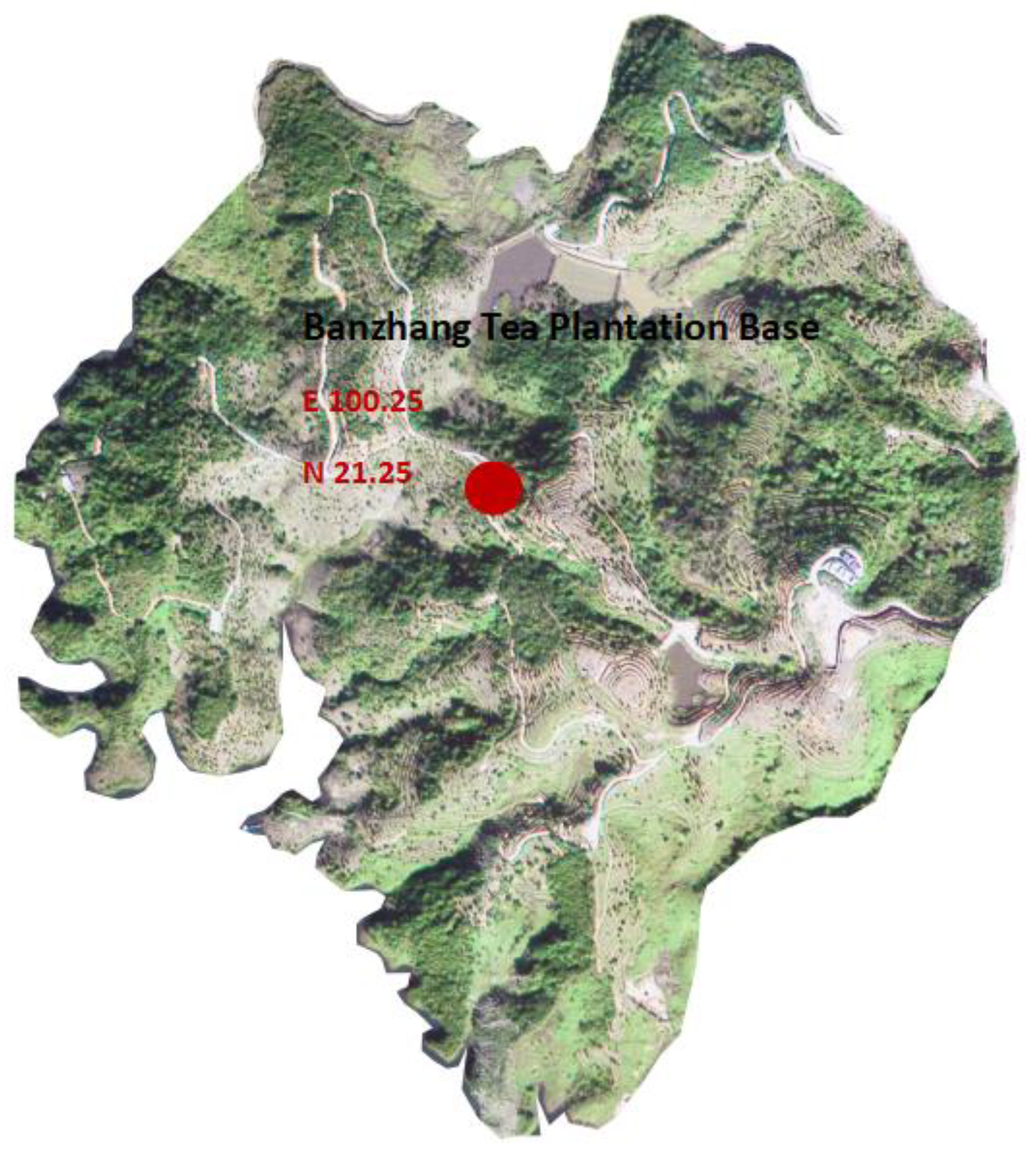
The study focuses on the relationship between soil conditions and the quality of Pu-erh tea, so it is necessary to obtain the soil environment data of the Pu-erh tea plantation base. The Pu-erh tea for the study came from the tea plantation base (
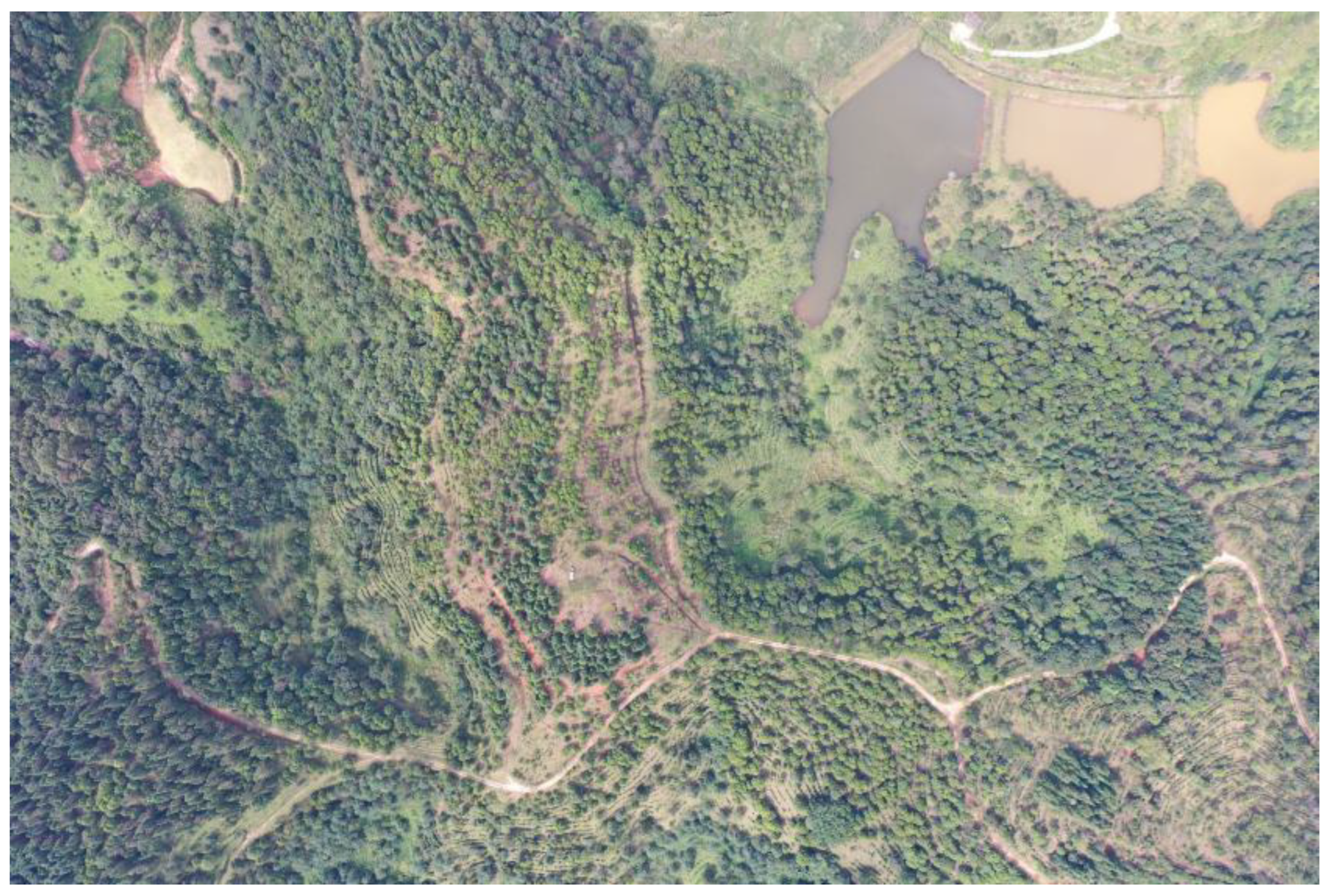
Figure 1.) in Menghai County, Xishuangbanna, Yunnan Province of China (Longitude 100.25, Latitude 21.25), The tea plantation base picture with drones is shown in
Figure 2.and the hour-by-hour data of soil temperature, soil humidity, and soil pH were obtained based on the meteorological station in Menghai County, with the data period from 1 June 2021, to 30 December 2021, which was obtained from the National Center for Meteorological Science and Technology. According to the study of tea Soil Environmental Quality, the soil environment data needed is the data of 15 days before picking, and the autumn tea picking time is from late September to the end of November, so the data time period used in this paper is from 5 September 2021, to 1 December 2021.
One bud and two new leaves were collected from the top, middle, and bottom of the slope in each slope direction to make sun-baked tea, and each sampling area was repeated three times. The sun-baked tea was used to determine the biochemical composition and to evaluate the sensory quality of the tea leaves. The soil collection area was between the tea picking site, and the topsoil of 4–5 cm of the soil surface was excavated, and the soil of the cultivation layer within 20 cm deep was taken vertically. The soil sample numbers are shown in
Table 1.
We conducted a preliminary screening of soil environmental factors, including soil pH, organic matter, and nutrient content in tea plantations, and the correlation coefficients are shown in
Figure 3. The formation of tea quality is closely related to the soil conditions, especially the soil environment conditions during the tea picking period directly affect the quality of tea, in which the average soil temperature, soil humidity, and soil pH in the first 15 days of the fresh leaf picking period are the main influencing factors.
- (1)
Temperature
The growing environment of high-quality Pu-erh tea belongs to a subtropical climate, where the year-round soil Kelvin temperature is maintained at about 288 k~300 k (15 °C~27 °C). If the temperature is lower or higher than this, the quality of Pu-erh tea produced will be very different.
- (2)
Humidity
The average annual rainfall of quality Pu’er tea mountains is maintained at 1200 mm to 1600 mm. Rainfall alone is not enough, but a certain amount of fog exposure is also needed, and the average annual fog exposure in quality Pu’er tea mountains ranges from 80 to 160 days. This provides favorable soil moisture nourishing conditions for the growth of Pu’er tea trees.
- (3)
Soil pH
The soils in China’s Yunnan Province are generally red loam, yellow loam, and brick red loam. In the Pu-erh tea-producing areas, suitable soils are loose, deep, well-drained, well-permeable, and slightly acidic soils with a pH value between 4 and 6. The average soil pH value in high-quality Pu-erh tea mountains is 4.5–5.5.
2.2. Methods
2.2.1. Tea Soil Environmental Quality Evaluation Method
Firstly, the soil element indexes that have an important influence on the key growth period of tea products are determined, the scoring threshold of each element is given, and then the comprehensive soil quality score of this tea product is calculated based on the influence weights of different soil environment elements, and finally, the soil environment quality is graded by combining with the physical and chemical index grading standard of Pu-erh tea.
denotes the tea soil environment quality evaluation index.
ai denotes the weights of average soil temperature, average soil relative humidity, and average soil pH value.
Mi denotes the average soil temperature, average soil relative humidity, and soil pH within 15 days of Pu-erh tea picking without the influence of agro-meteorological disasters (
Table 2). The range of
ai,
Mi coefficients in the model can be set according to the actual situation of the tea plantation.
2.2.2. Tea Soil Environmental Quality Grade Classification
According to the Soil Environmental Quality index of tea, we divided the tea climatic taste evaluation grade into four categories. It is shown in
Table 3 below.
The research firstly obtains the required dataset of soil conditions, analyzes the soil factors affecting tea quality by reviewing the data, determines the Soil Environmental Quality evaluation model according to the climatic factors, and classifies the tea quality into grades to facilitate our further in-depth learning research.
2.2.3. Deep Learning Methods
The application of deep learning, an emerging machine learning technique, has brought machine learning closer and closer to the original purpose of artificial intelligence, and its advantages are great in the fields of speech and image recognition [
42]. Deep learning allows machines to simulate behaviors such as seeing, hearing, and thinking, thus solving a large number of pattern recognition problems and enabling significant advances in artificial intelligence technology [
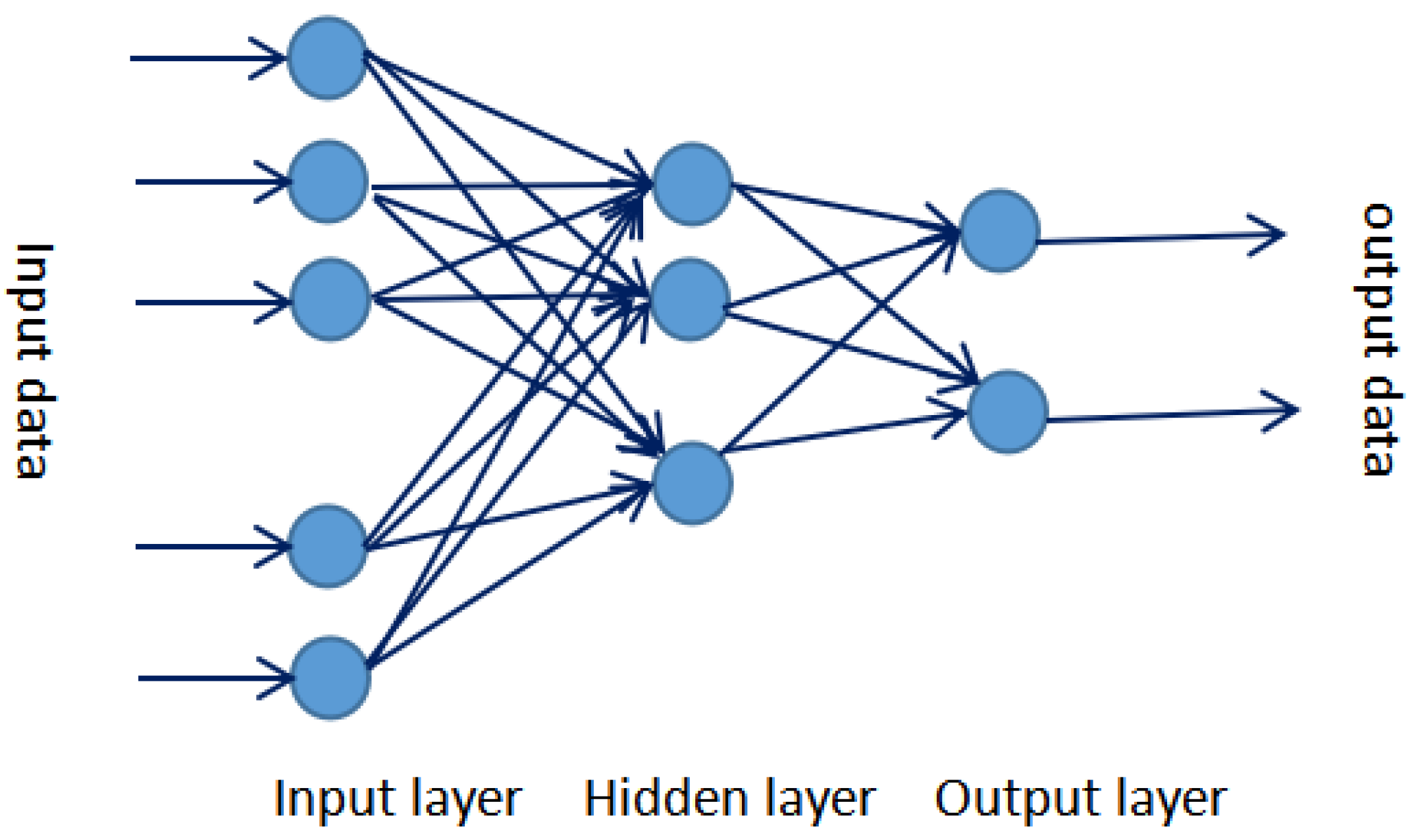
43]. Deep learning does not refer specifically to a particular algorithm, but is a generic term for a class of neural network learning [
44], and deep learning is an effective application-oriented practical approach [
45], the deep learning neural network model is shown in
Figure 4.
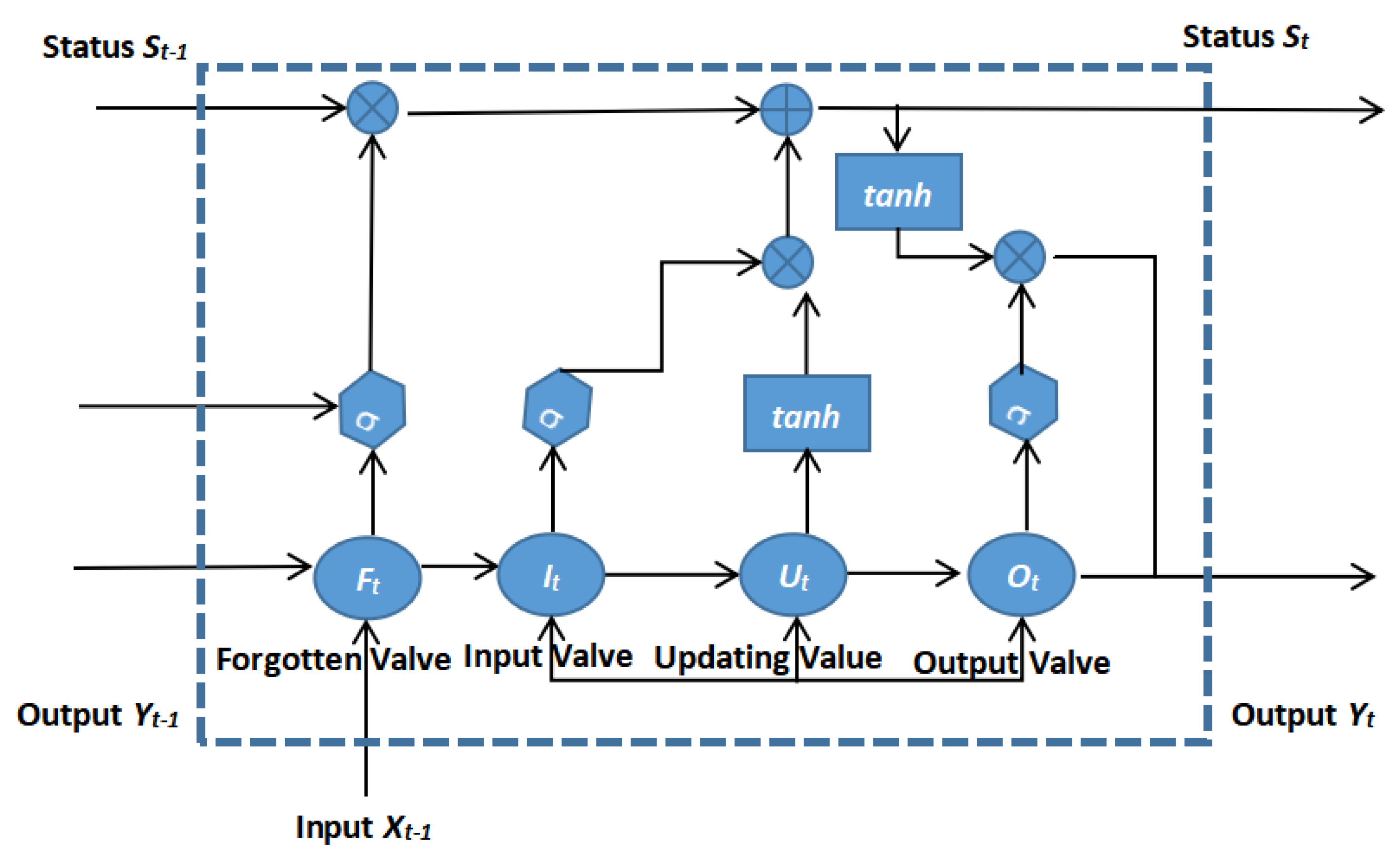
Long Short Term Memory (LSTM) is designed to address the gradient disappearance and explosion problems that arise when RNNs learn background information at large intervals, and its memory modules are added to the structure. These modules can be thought of as memory chips in a computer, each with a number of cyclically linked memory cells and three gates (input, output, and forget, equivalent to write, read, and reset). Only in each gate can information interact with neurons, so it is important to learn how to open and close these gates so that gradients do not explode or disappear. The extent to which past and present information is remembered and forgotten is controlled by these control gates, which gives the recurrent neural network a long-term memory function and the ability to use long-spaced information to solve current problems. Its structure is shown in
Figure 5.
The forgetting valve
(Forget Gate) Sigmoid activation function is used to control the amount of state S
t-1 input from the previous step to the current step, i.e., the degree to which the state of the previous step is forgotten, and its input is the output
of the previous step and the input
Xt of this step. The valve is calculated as follows:
The input valve (Input Gate) is used for input to the current state. This input valve uses the Sigmoid activation function to determine the current output value
Y on the one hand, and the tanh function to generate the current candidate vector
on the other hand, and this update valve decides whether to add this vector to the current state
. Such a valve is calculated as follows.
Update Gate
(Update Gate) determines whether the current unit should be updated from
to
state by multiplying the forgotten valve by the output valve. This valve is calculated according to the following method.
Output Valve
is used to determine the current cell state by analyzing the output value of the old cell and the input of the current cell using the Sigmoid activation function. Then, the current unit state
is processed by the tanh function and multiplied with the output
of the Sigmoid activation function, and finally, the output value
of the current unit is determined.
In the above equation, is the weight; is the parametric vector; is the Sigmoid activation function; is the hyperbolic tangent activation function.
3. Results
3.1. LSTM-Based Soil Environmental Quality Classification Model for Pu-erh Tea
The hardware experimental environment for the study is DESKTOP-96BC8BT, Intel(R) Core(TM) i5-10210U CPU @ 1.60 GHz (8 CPUs), 2.11 GHz, 8192 MB RAM, Windows 11 Professional Edition 22000.613 operating system. The software environment for the experiment is Python 3.7, The development tool is PyCharm2019.3.3x64.
From the previous study, we can conclude that the average soil temperature, average soil humidity, and soil pH are the main characteristics that affect the quality of tea leaves. However, the hour-by-hour temperature, humidity, and pH are available in the obtained meteorological data set, so data processing is also needed to calculate the average soil temperature, average soil humidity, and average soil pH for the 15 days before the picking date. After getting the processed features, it is necessary to classify the tea quality level. According to Equation (1) of the tea Soil Environmental Quality evaluation model, the assignment process is carried out to calculate the tea quality grade, and the implementation code of Average soil temperature assignment is as follows.
The code implementation of the average soil humidity assignment calculation is as follows:
if U >= 40:
M_list.append (3)
elif 30 <= U < 40:
M_list.append (2)
elif 20 <= U < 30:
M_list.append (1)
else:
M_list.append (0)
The code implementation of the soil pH calculation is as follows:
if 4.5 <= P < = 5.5:
M_list.append(3)
elif 5.5 <= P <= 6.5
M_list.append(2)
elif 6.5 < P <= 7.5
M_list.append(1)
else:
M_list.append(0)
Return M_list
According to
Table 2, the grade classification of tea quality is implemented with the following code.
def change_I (i):
if i >= 2.5:
return ’Special Grade’
elif 1.5 <= i < 2.5:
return ’Excellent Grade’
elif 0.5 <= i < 1.5:
return ’Good Grade’
else:
return ’General grade’
3.2. Training Model
The prediction task studied is a tea Soil Environmental Quality class classification task on time series, constructed using a neural network model of LSTM. A model is built using Keras. Sequential, which can easily stack multiple layers on top of each other. In the model structure, the LSTM layer consists of 50 neurons, and each layer is combined with a Dropout layer, which allows the output of randomly selected neurons to be ignored during training, thus reducing the sensitivity of individual neurons to certain weights and thus avoiding overfitting of the model. To prevent overfitting with guaranteed model accuracy, we usually set the dropout_rate to 20%. Add a relu activation function to the last layer of the fully connected layer. The following is the code to create the LSTM model.
def create_model (input_length):
model = Sequential ( )
model.add (LSTM (units = 50, return_sequences = True, input_shape = (input_length,1)))
model.add (Dropout (0.2))
model.add (LSTM (units = 50, return_sequence = False))
model.add (Dropout (0.2))
model.add (Dense(1, activation=’relu’))
Before the model is trained, the dataset needs to be divided into a training set and a test set. To better evaluate the performance of the model, the training set can be divided into a training set and a validation set. The training dataset is used to run the learning algorithm and train the model. The validation dataset can be used for model tuning, EarlyStopping, feature selection, etc. to select a suitable model. The test dataset is used to evaluate the performance of the selected model, but no corresponding changes are made to the learning algorithm or parameters.
In the experiments of this paper, 90% of the dataset is divided into a training set, 10% is divided into a test set, and then 10% of the training set is divided into a validation set. The model is trained by passing in the training set x, the training set label y, using the fit (fitting) method, and then splitting 10% of the validation set from the training set as a measure of early stopping. Where epochs are the number of iterations and batch_size is the number of training samples randomly sampled at each epoch. The implementation code is as follows, and the structure of the output LSTM model is shown in
Figure 6.
model = create_model (len (X_train [0]))
hist = model.fit (X_train, y_train, batch_size = 2, validation_split = 0.1, epochs = 200, shuffle = False, verbose = 1)
The final output model structure is a two-layer LSTM with one fully connected layer, specifying the number of neurons in the LSTM layer as 50, the number of parameters in the first LSTM layer as 10,400, the number of parameters in the second LSTM layer as 20,200, and the number of parameters in the fully connected layer as 51, for a total number of parameters in this model of 30,651.
4. Model Evaluation
The goal of machine learning is to minimize the loss function, not only to have a good predictive ability for the training data during the learning process but also to have a good predictive ability for the test set. To evaluate the model fitting effect, it is often expressed as underwriting, good fitting, and overfitting. Generally, a model that fits well has better generalization ability and has a better effect on the test set.
4.1. The Loss Function
The loss function is used to evaluate the difference between the prediction of the model and the actual value, and the deep learning model is used to calculate the loss function and update the model parameters so as to reduce the optimization error until the loss function value decreases to the target value or the training count is reached. Due to the different models, their loss functions are not the same.
Mean Square Error (MSE) is evaluated as the average of the squared difference between the predicted and actual values of the model, and the lower the MSE value, the better the performance of the prediction model. Its calculation is shown in (8).
where
y is the expected output,
is the predicted value of the deep learning model, and
N is the amount of information in a batch.
Mean Absolute Error (MAE) is used to measure the average of the absolute sum of the difference between the model prediction and the true value, which can be considered as the average error in the generic form. The MAE method can avoid generating positive and negative errors that cancel each other and therefore can reflect the degree of error more accurately. Its calculation Formula (9) shows.
Root Mean Squad Error (RMSE) is in essence the same as MSE, which is an expression of the MSE open root sign for a better description of the data. The calculation formula is shown in Equation (10).
4.2. Model Compilation
Deep learning is the learning goal of deep learning, which is to learn a “good” model to make decisions, usually, the error between the predicted value and the target value is as low as possible, and the function to measure this error is called the loss function. For different tasks, different loss functions are often needed to measure, and this paper uses the mean squared loss function for the regression task.
When the learning goal of deep learning is to greatly, reduce a certain loss function, however, the loss function of machine learning models is more complex, and it is difficult to directly find the formula solution for minimizing the loss function, then we can optimize the model parameters by finite iterations of optimization algorithms (such as gradient descent, stochastic gradient descent, Adam, etc.) to reduce the value of the loss function as much as possible and obtain a better parameter value. In this paper, we use the Adam optimization algorithm, which is a collection of the advantages of two stochastic gradient descents.
4.3. Model Predictive Analysis
MSE and MAE can be used as both the loss function and the indicator function. In this paper, MSE is used as a loss function and MAE is used as an indicator function to compare the model prediction effect in the study of tea soil environmental quality classification task.
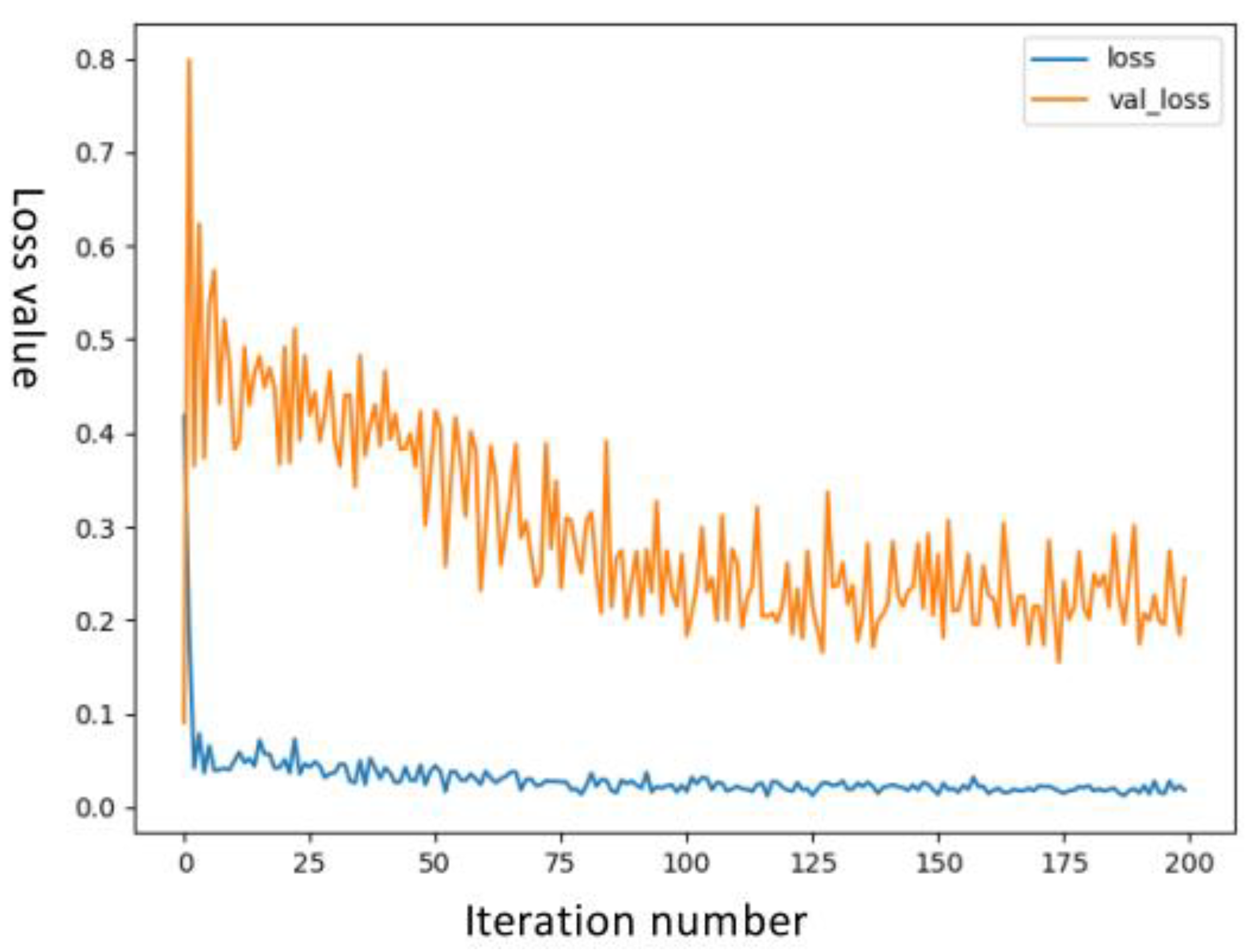
Figure 7 shows the resulting graph of MSE as a loss function, MSE has a low error on the training set, and validation set, the image tends to be smooth and the deviation on the training and validation set is small.
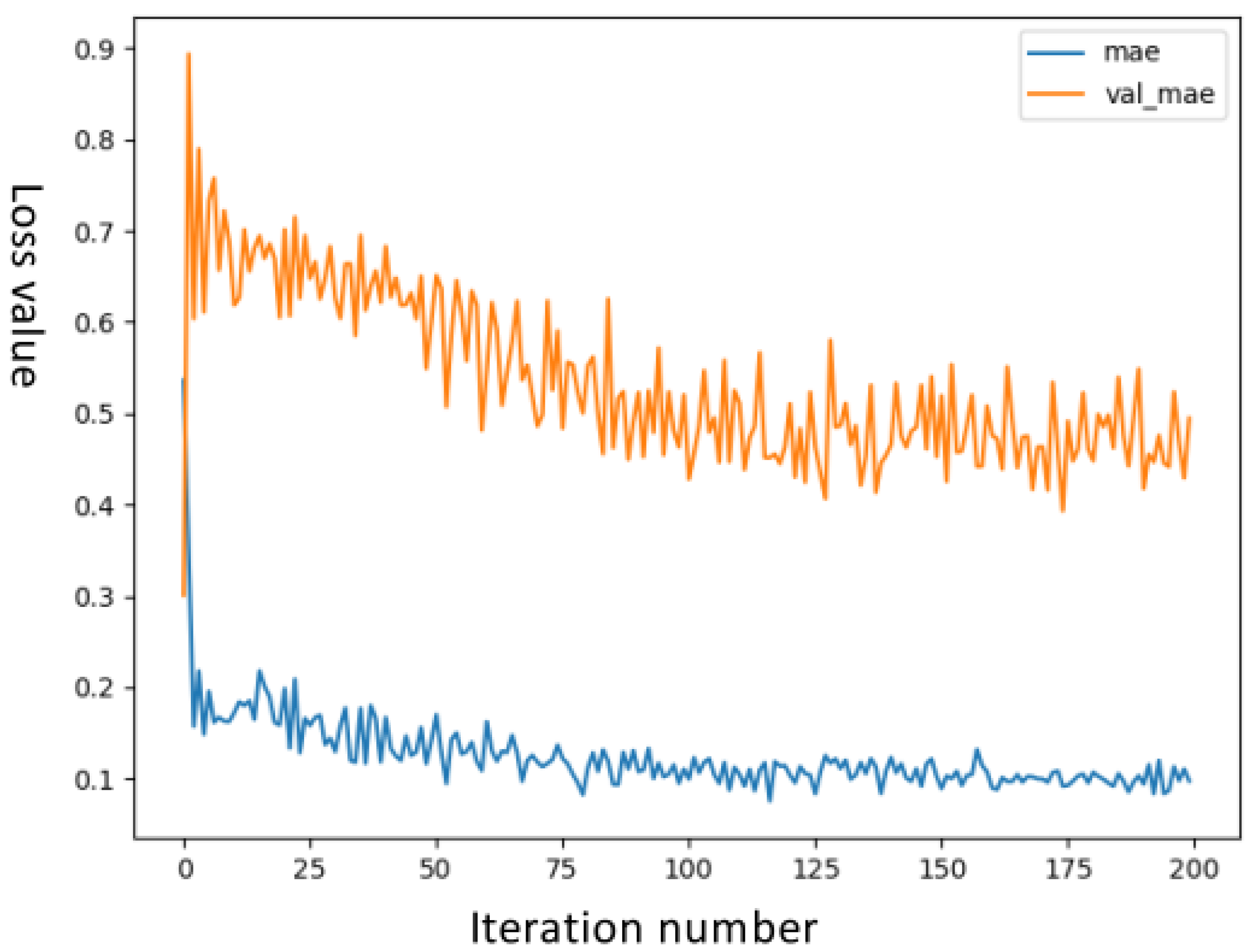
Figure 8 shows the plot of MAE as a function of the model’s metric, compared with the MSE images. The errors on the MAE training and validation sets are lower, the images tend to be smoother, and the deviations on the training and validation sets are smaller.
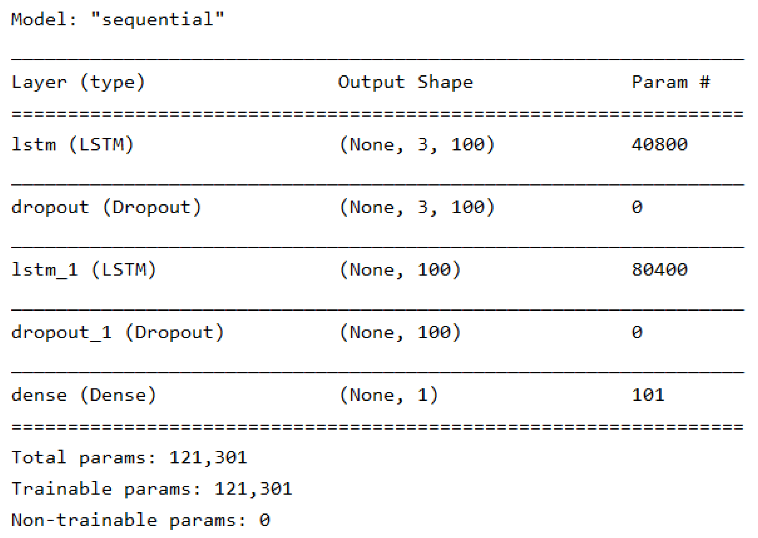
In order to study a model that is more suitable for this experiment, the LSTM model is compared with the previous model results by adjusting the parameters of the LSTM model. The LSTM neurons in each layer were adjusted to 100, and the Dropout layer was set to 15%, and the code for adjusting the parameters was as follows, and the structure of the LSTM model is shown in
Figure 9.
def.create_model (input_length):
model=Sequential ()
model.add (LSTM(units = 100,return_sequences = True, input_shape = (input_length,1)))
model.add (Droput(0.15))
model.add (LSTM(units = 100, return_sequences = False))
model.add (Dropout(0.15))
model.add (Dense (1,activation = ’relu’))
The output of the LSTM model after adjusting the parameters is shown in
Figure 7. The number of neurons in the LSTM layer is 100, the number of parameters in the first LSTM layer is 40,800, the number of parameters in the second LSTM layer is 80,400, and the number of parameters in the fully connected layer is 101, and the total number of parameters in this model is 12,301.
Figure 10 shows the resulting graph of MSE as loss function loss after adjusting the parameters. The value of MSE is the low error on the training set, and validation set, the image tends to be smooth, and the deviation on the training and validation sets is small, which indicates that the model has a good prediction effect.
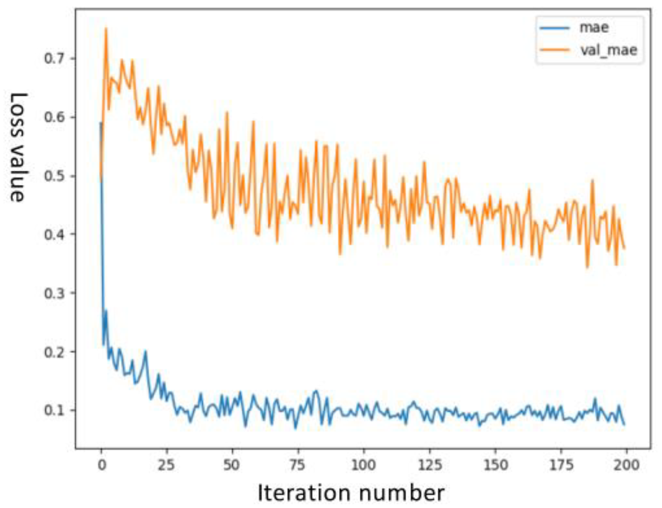
Figure 11 shows the plot of the indicator function using MAE as a model after adjusting the parameters and comparing it with the MSE image. The errors on the MAE training and validation sets are lower, the images tend to be smooth, and the deviations on the training and validation sets are smaller, indicating that the model predicts well.
Due to the randomness introduced in this model, the values of MSE and RMSE vary with the number of runs, but the differences are not large, and the values in
Table 4 above are compared by taking the average value after 10 runs. The neurons of the first set of LSTM model parameters are 50 and the dropout is 0.2, and the neurons of the second set of LSTM model parameters are 100 and the dropout is 0.15. Comparing the values of MSE and RMSE of LSTM using the two sets of parameters, it can be concluded that the values of MSE and RMSE are smaller when using the second set of parameters, indicating that the prediction effect of the model after adjusting the parameters has significantly improved.
Classification of Pu-erh tea Soil Environmental Quality classes is performed using a model of LSTM, which is suitable for tasks dealing with time series. Each prediction process is introduced one by one in conjunction with the complete process of prediction. From data processing to model construction and final prediction results, each step is explained conceptually as well as programmed using Python language, suitable learning objectives and optimization algorithms are selected, prediction models are evaluated through model evaluation metric, and finally, a better model is selected after the model comparison.
5. Model Comparison Analysis
5.1. Random Forest Model
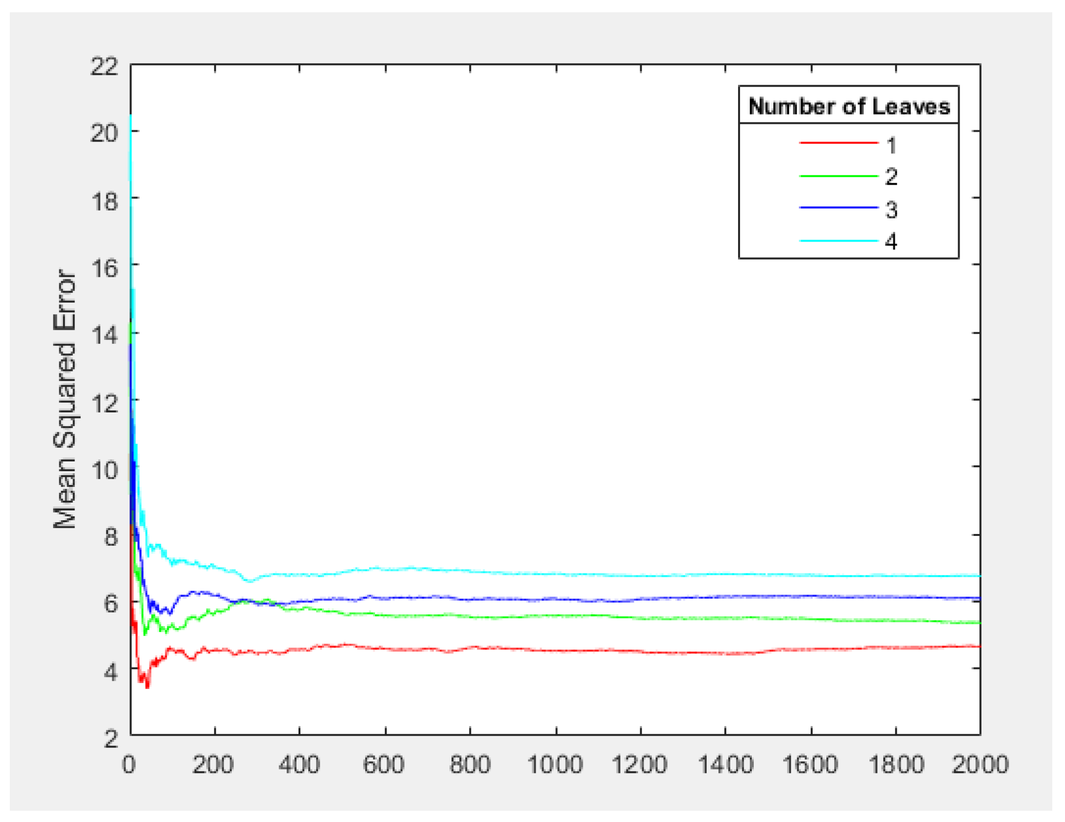
The construction of a random forest consists of three parts, the generation of a training set, the construction of a decision tree, and the formation of the algorithm. First, a training set is generated by the bootstrap method, then for each training set, a decision tree is constructed, and when the nodes find features for splitting, a portion of the features are randomly selected among the features, and the optimal solution is found among the selected features and applied to the nodes and split. The average soil temperature, average soil moisture, and average pH were used as input features to train the samples for analysis, and the results were obtained as shown in
Figure 12.
From
Figure 12, it can be seen that the number of leaf nodes of the model is taken as 1, 2, 3, and 4 for training respectively, and the MSE is the lowest when the number of leaf nodes is 1, and it starts to smoothly stop declining when it reaches 80, so it is more appropriate to choose the number of leaf nodes of the random forest model as 1 and the number of decision trees as 80.
The selected soil environment factors are used as the input variable matrix of the model, and the soil environment classification level is used as the output variable. The input variable matrix and the output variable together form the training data set, and the training data set is constructed and formed. When each node of the regression tree is split, the input parameters are randomly selected as the splitting subset of the current node, and the node is split using the CART method in each subset. Each regression tree is split from top to bottom until it reaches a leaf node with an estimated value, and all regression trees form a random forest.
The final rank estimation result is obtained by averaging the soil environmental rank output from all regression trees to generate the random forest model. The vector of attribute parameters in the prediction data set is input into the trained prediction model, and the predicted values of each individual regression tree are averaged using the “simple averaging method” to obtain the predicted values of soil environment classification.
5.2. BP Neural Network Model
The back propagation neural network (BP) is a multi-layer feed-forward neural network trained according to the error backpropagation algorithm. It mainly consists of an input layer, a hidden layer, and an output layer. The input layer passes the stimulus to the invisible layer, which does not operate on the input signal and has no associated weight or bias value. The invisible layer passes the stimulus to the output layer through the weight and activation function of the association between neurons, which does not receive signals directly from the outside world and does not send signals directly to the outside world, and can have multiple layers. The output layer is the last layer of the network, which receives the signal from the last invisible layer and outputs the predicted value of the final model, as
Figure 13.
The first part shows the graph of the training parameters of the BP neural network, from which it can be seen that the input layer has four neural nodes, the output layer has 1 neural node, and the invisible layer has six neural nodes. The second part shows the training algorithm. The Levenberg-Marquardt (L-M) algorithm is chosen as the training algorithm, which has both the fast local convergence of Newton’s method and the ideal overall convergence. The third section shows the training progress. Epoch is the number of training passes. All the data are passed in one positive direction and one negative direction to become an epoch, the maximum number of trainings can be set independently, this training is set to 10,000, the specific training number is shown in the progress bar as epoch 11 when the BP neural network has the best training results. Time shows the training process time. Performance indicates the performance index. This training refers to the maximum value of the mean square error (MSE), the maximum number of times the MSE can be trained can be set independently, and the progress bar shows the current mean square error, if the mean square error at a certain point in the training process is smaller than the set value, the training will be automatically suspended, can be set with the train goal parameter. The gradient value can be set independently on the right side of the progress bar, and the progress bar shows the current gradient value. If the current gradient value reaches the autonomous value, the training will be paused automatically.
5.3. Comparative Analysis of Models
Comparing the three prediction models, it can be seen from
Table 5. that the LSTM-based model has the best prediction results, the BP neural network-based model has the second best prediction results, and the random forest-based prediction model has the worse prediction results.
The coefficient of determination of the random forest-based prediction model was 0.89. The mean absolute error (MAE) was 2.93, the mean square error (MSE) was 9.95, the mean absolute percentage error (MAPE) was 0.038, and the root mean square error (RMSE) was 3.15. The resultant coefficient of determination R2 of the BP neural network-based prediction model was 0.91 the mean absolute error (MAE) was 7.14, the mean square error (MSE) was 20.36, the mean absolute percentage error (MAPE) was 0.078, and the root mean square error (RMSE) was 8.31. The LSTM model achieves the best results within the set parameters with the training data corresponding to an R-value of 0.99869. The coefficient of determination R2 of the prediction results of the BP neural network-based prediction model is 0.95, indicating a good fit. The results were a mean absolute error (MAE) of 1.55, mean square error (MSE) of 0.090, mean absolute percentage error (MAPE) of 0.0198, and root mean square error (RMSE) of 0.300.
6. Conclusions
The main research objectives of this paper are divided into the following points. To analyze the techniques related to deep learning and the models based on deep learning, and to design an algorithmic model suitable for this research paper, as well as the algorithms used in this model. (2) To select a Pu-erh tea environmental quality model suitable for this research paper based on the existing tea Soil Environmental Quality evaluation models. (3) Screen the soil characteristic factors related to tea quality from the tea garden data and select the appropriate characteristics to calculate the tea Soil Environmental Quality Index. (4) Establish the model, select the relevant data and write the program, build the model with a suitable algorithm, evaluate the algorithm according to the prediction results, and classify the tea Soil Environmental Quality by grade.
This paper focuses on the LSTM-based classification of Pu-erh tea Soil Environmental Quality classes, firstly calculating the tea Soil Environmental Quality index, then dividing the dataset into a training set, testing set, and validation set, and creating an LSTM model to predict. The model has two LSTM layers and one fully connected layer, which has some advantages in dealing with time series data with long-term memory function and combined with the Dropout layer in the middle to prevent overfitting. Finally, the MAE and MSE of the model on both training and validation sets are low, and the model has a better prediction effect. The paper also compares two other machine learning algorithms, based on BP neural network and random forest prediction model, by evaluating the coefficient of determination (R2), mean absolute error (MAE), mean square error (MSE), mean absolute percentage error (MAPE) and root mean square error (RMSE) comparing the best prediction model based on LSTM neural network, with R2 of 0.95, MAE of 1.55, MSE of 0.090, MAPE of 0.0198, and RMSE of 0.3. The LSTM solves the long-term dependence problem of RNN to some extent, but it is not enough, and it still seems tricky when dealing with longer sequences, so the research model in this paper is not suitable for dealing with excessively long data, which is computationally time-consuming and does not achieve good results, and we hope to further study the prediction model that is more suitable for long sequences.
The superior soil conditions create suitable growing conditions for growing tea, and also lay the foundation for the rich inclusions of Pu’er tea. The paper innovatively proposes to introduce the main inclusions of Pu’er tea into the classification and discrimination model of the soil environment of tea plantations, while using machine learning-related algorithms to classify and predict the categories of soil environmental quality instead of relying solely on statistical data for analysis. This research work makes it possible to quickly and accurately determines the physiological status of tea leaves based on the establishment of a soil environment quality prediction model, which provides effective data for the intelligent management of tea plantations and has the advantage of rapid and low-cost assessment compared with the need to measure the intrinsic quality of Pu-erh tea after harvesting is completed.
Author Contributions
W.Y., X.L., X.W., Y.C. and X.D. prepared the data layers, figures, and tables; Q.W., K.H., Z.C. and W.W. performed the experiments and analyses. X.C. and B.W. supervised the research, finished the first draft of the manuscript, edited and reviewed the manuscript, and contributed to the model construction and verification. All authors have read and agreed to the published version of the manuscript.
Funding
This work is supported by the Yunnan Science and Technology Major Project (No. 202002AE09001004), the National Natural Science Foundation of China (No. 32060702), the Yunnan Provincial Basic Research Project (No. 202101AT070267), the scientific research fund project of Kunming Metallurgy College (No. 2020XJZK01), the Scientific research fund project of Yunnan Provincial Education Department (No. 2021J0943), the Yunnan Province “Ten Thousand People Plan” Industrial Technology Leading Talents Project (No. YNWR-CYJS-2018-009), and the Yunnan Province Technology Innovation Talent Project (No.2019BH089).
Conflicts of Interest
The authors declare no conflict of interest.
References
- Lee, L.K.; Foo, K.Y. Recent advances on the beneficial use and health implications of Pu-Erh tea. Food Res. Int. 2013, 53, 619–628. [Google Scholar] [CrossRef]
- Liu, J.Y.; He, D.; Xing, Y.F.; Zeng, W.; Ren, K.; Zhang, C.; Lu, Y.; Yang, S.; Ou, S.-J.; Wang, Y.; et al. Effects of bioactive components of Pu-erh tea on gut microbiomes and health: A review. Food Chem. 2021, 353, 129439. [Google Scholar] [CrossRef] [PubMed]
- Zhang, Z.; He, F.; Yang, W.; Yang, L.; Huang, S.; Mao, H.; Hou, Y.; Xiao, R. Pu-erh tea extraction alleviates intestinal inflammation in mice with flora disorder by regulating gut microbiota. Food Sci. Nutr. 2021, 9, 4883–4892. [Google Scholar] [CrossRef]
- Ge, Y.; Li, N.; Fu, Y.; Yu, X.; Xiao, Y.; Tang, Z.; Wu, J.L.; Jiang, Z.H. Deciphering superior quality of Pu-erh tea from thousands of years’ old trees based on the chemical profile. Food Chem. 2021, 358, 129602. [Google Scholar] [CrossRef]
- Chan EW, C.; Wong, S.K.; Chan, H.T. An overview of Pu-erh tea and its health-promoting effects of lipid-lowering and anti-obesity. J. Chin. Pharm. Sci. 2021, 30, 11. [Google Scholar]
- Hong, Z.; Zhang, C.; Kong, D.; Qi, Z.; He, Y. Identification of storage years of black tea using near-infrared hyperspectral imaging with deep learning methods. Infrared Phys. Technol. 2021, 114, 103666. [Google Scholar] [CrossRef]
- Yang, Z.; Gao, J.; Wang, S.; Wang, Z.; Li, C.; Lan, Y.; Sun, X.; Li, S. Synergetic application of E-tongue and E-eye based on deep learning to discrimination of Pu-erh tea storage time. Comput. Electron. Agric. 2021, 187, 106297. [Google Scholar] [CrossRef]
- Chen, J.; Jia, J. Automatic Recognition of Tea Diseases Based on Deep Learning. In Advances in Forest Management under Global Change; IntechOpen: London, UK, 2020; 180p, Available online: https://www.intechopen.com/books/9720 (accessed on 27 September 2022). [CrossRef]
- Latha, R.S.; Sreekanth, G.R.; Suganthe, R.C.; Rajadevi, R.; Karthikeyan, S.; Kanivel, S.; Inbaraj, B. Automatic detection of tea leaf diseases using deep convolution neural network. In Proceedings of the 2021 International Conference on Computer Communication and Informatics (ICCCI), IEEE, Coimbatore, India, 27–29 January 2021; pp. 1–6. [Google Scholar]
- Kamrul, M.H.; Rahman, M.; Robin MR, I.; Hossain, M.S.; Hasan, M.H.; Paul, P. A deep learning based approach on categorization of tea leaf. In Proceedings of the International Conference on Computing Advancements, Dhaka, Bangladesh, 10–12 January 2020; pp. 1–8. [Google Scholar]
- Chen, J.; Liu, Q.; Gao, L. Visual tea leaf disease recognition using a convolutional neural network model. Symmetry 2019, 11, 343. [Google Scholar] [CrossRef] [Green Version]
- Sun, X.; Mu, S.; Xu, Y.; Cao, Z.; Su, T. Image recognition of tea leaf diseases based on convolutional neural network. In Proceedings of the 2018 International Conference on Security, Pattern Analysis, and Cybernetics (SPAC), IEEE, Jinan, China, 14–17 December 2018; pp. 304–309. [Google Scholar]
- Zhang, Y.D.; Muhammad, K.; Tang, C. Twelve-layer deep convolutional neural network with stochastic pooling for tea category classification on GPU platform. Multimed. Tools Appl. 2018, 77, 22821–22839. [Google Scholar] [CrossRef]
- Jiang, P.; Chen, Y.; Liu, B.; He, D.; Liang, C. Real-Time Detection of Apple Leaf Diseases Using Deep Learning Approach Based on Improved Convolutional Neural Networks. IEEE Access 2019, 7, 59069–59080. [Google Scholar] [CrossRef]
- Yang, H.; Chen, L.; Chen, M.; Ma, Z.; Deng, F.; Li, M.; Li, X. Tender tea shoots recognition and positioning for picking robot using improved YOLO-V3 model. IEEE Access 2019, 7, 180998–181011. [Google Scholar] [CrossRef]
- Cai, L.; Barneche, A.M.; Herbout, A.; Foo, C.S.; Lin, J.; Chandrasekhar, V.R.; Aly, M.M.S. TEA-DNN: The quest for time-energy-accuracy co-optimized deep neural networks. In Proceedings of the 2019 IEEE/ACM International Symposium on Low Power Electronics and Design (ISLPED), IEEE, Lausanne, Switzerland, 29–31 July 2019; pp. 1–6. [Google Scholar]
- Hu, G.; Fang, M. Using a multi-convolutional neural network to automatically identify small-sample tea leaf diseases. Sustain. Comput. Inform. Syst. 2022, 35, 100696. [Google Scholar] [CrossRef]
- Paranavithana, I.R.; Kalansuriya, V.R. Deep convolutional neural network model for tea bud (s) classification. IAENG Int. J. Comput. Sci. 2021, 48, 599–604. [Google Scholar]
- Paul, A.; Bhattacharyya, S.; Chakraborty, D. Estimation of Shade Tree Density in Tea Garden using Remote Sensing Images and Deep Convolutional Neural Network. J. Spat. Sci. 2021, 1–15. [Google Scholar] [CrossRef]
- Tang, Z.; Li, M.; Wang, X. Mapping tea plantations from VHR images using OBIA and convolutional neural networks. Remote Sens. 2020, 12, 2935. [Google Scholar] [CrossRef]
- Qi, C.; Gao, J.; Pearson, S.; Harman, H.; Chen, K.; Shu, L. Tea chrysanthemum detection under unstructured environments using the TC-YOLO model. Expert Syst. Appl. 2022, 193, 116473. [Google Scholar] [CrossRef]
- Yang, H.; Chen, L.; Ma, Z.; Chen, M.; Zhong, Y.; Deng, F.; Li, M. Computer vision-based high-quality tea automatic plucking robot using Delta parallel manipulator. Comput. Electron. Agric. 2021, 181, 105946. [Google Scholar] [CrossRef]
- Li, Y.; He, L.; Chen, J.; Lv, J.; Wu, C. High-efficiency tea shoot detection method based on a compressed deep learning model. Int. J. Agric. Biol. Eng. 2022, 15. [Google Scholar]
- Tian, J.; Zhu, H.; Liang, W.; Chen, J.; Wen, F.; Long, Z. Research on the Application of Machine Vision in Tea Autonomous Picking. In Journal of Physics: Conference Series; IOP Publishing: Bristol, UK, 2021; Volume 1952, p. 022063. [Google Scholar]
- Gong, T.; Wang, Z.L. A tea tip detection method suitable for tea pickers based on YOLOv4 network. In Proceedings of the 2021 3rd International Symposium on Robotics & Intelligent Manufacturing Technology (ISRIMT), IEEE, Changzhou, China, 24–26 September 2021; pp. 264–268. [Google Scholar]
- Cheng, E.S.; Yang, J.Y.; Lee, J.D.; Chen, K.Y.; Hu, N.Z.; Chen, L.Y. AIoT module development for automated production. In Proceedings of the 2021 IEEE International Conference on Consumer Electronics-Taiwan (ICCE-TW), IEEE, Penghu, Taiwan, 15–17 September 2021; pp. 1–2. [Google Scholar]
- Xu, W.; Zhao, L.; Li, J.; Shang, S.; Ding, X.; Wang, T. Detection and classification of tea buds based on deep learning. Comput. Electron. Agric. 2022, 192, 106547. [Google Scholar] [CrossRef]
- Wang, X.V.; Pinter, J.S.; Liu, Z.; Wang, L. A machine learning-based image processing approach for robotic assembly system. Procedia CIRP 2021, 104, 906–911. [Google Scholar] [CrossRef]
- He, H.; Shi, L.; Yang, G.; You, M.; Vasseur, L. Ecological risk assessment of soil heavy metals and pesticide residues in tea plantations. Agriculture 2020, 10, 47. [Google Scholar] [CrossRef] [Green Version]
- Yun, M.; Shan, J.; Chunfeng, F.; Mengze, Z.; Xiaodong, J. A study and implement of Tea QS Trace System based on WebGIS. In Proceedings of the 2011 International Conference on Electronics, Communications and Control (ICECC), IEEE, Ningbo, China, 9–11 September 2011; pp. 1281–1284. [Google Scholar]
- Tresch, S.; Moretti, M.; Le Bayon, R.C.; Mäder, P.; Zanetta, A.; Frey, D.; Stehle, B.; Kuhn, A.; Munyangabe, A.; Fliessbach, A. Urban soil quality assessment—A comprehensive case study dataset of urban garden soils. Front. Environ. Sci. 2018, 6, 136. [Google Scholar] [CrossRef]
- Cao, H.; Qiao, L.; Zhang, H.; Chen, J. Exposure and risk assessment for aluminium and heavy metals in Puerh tea. Sci. Total Environ. 2010, 408, 2777–2784. [Google Scholar] [CrossRef]
- Zhang, J.; Yang, R.; Chen, R.; Peng, Y.; Wen, X.; Gao, L. Accumulation of heavy metals in tea leaves and potential health risk assessment: A case study from Puan County, Guizhou Province, China. Int. J. Environ. Res. Public Health 2018, 15, 133. [Google Scholar] [CrossRef] [PubMed] [Green Version]
- Karak, T.; Bora, K.; Paul, R.K.; Das, S.; Khare, P.; Dutta, A.K.; Boruah, R.K. Paradigm shift of contamination risk of six heavy metals in tea (Camellia sinensis L.) growing soil: A new approach influenced by inorganic and organic amendments. J. Hazard. Mater. 2017, 338, 250–264. [Google Scholar] [CrossRef]
- Liu, Y.J.; Zhu, Y.G.; Ding, H. Lead and cadmium in leaves of deciduous trees in Beijing, China: Development of a metal accumulation index (MAI). Environ. Pollut. 2007, 145, 387–390. [Google Scholar] [CrossRef]
- Pławiak, P.; Maziarz, W. Classification of tea specimens using novel hybrid artificial intelligence methods. Sens. Actuators B: Chem. 2014, 192, 117–125. [Google Scholar] [CrossRef]
- Gayathri, S.; Wise DJ, W.; Shamini, P.B.; Muthukumaran, N. Image analysis and detection of tea leaf disease using deep learning. In Proceedings of the 2020 International Conference on Electronics and Sustainable Communication Systems (ICESC), IEEE, Coimbatore, India, 2–4 July 2020; pp. 398–403. [Google Scholar]
- Khanali, M.; Mobli, H.; Hosseinzadeh-Bandbafha, H. Modeling of yield and environmental impact categories in tea processing units based on artificial neural networks. Environ. Sci. Pollut. Res. 2017, 24, 26324–26340. [Google Scholar] [CrossRef]
- Kimutai, G.; Ngenzi, A.; Said, R.N.; Kiprop, A.; Förster, A. An optimum tea fermentation detection model based on deep convolutional neural networks. Data 2020, 5, 44. [Google Scholar] [CrossRef]
- Sitienei, B.J.; Juma, S.G.; Opere, E. On the use of regression models to predict tea crop yield responses to climate change: A case of Nandi East, sub-county of Nandi county, Kenya. Climate 2017, 5, 54. [Google Scholar] [CrossRef] [Green Version]
- Liu, Y.; Heuvelink, G.B.; Bai, Z.; He, P.; Xu, X.; Ding, W.; Huang, S. Analysis of spatio-temporal variation of crop yield in China using stepwise multiple linear regression. Field Crops Res. 2021, 264, 108098. [Google Scholar] [CrossRef]
- Phan, P.; Chen, N.; Xu, L.; Chen, Z. Using multi-temporal MODIS NDVI data to monitor tea status and forecast yield: A case study at Tanuyen, Laichau, Vietnam. Remote Sens. 2020, 12, 1814. [Google Scholar] [CrossRef]
- Guo, Y.; Liu, Y.; Oerlemans, A.; Lao, S.; Wu, S.; Lew, M.S. Deep learning for visual understanding: A review. Neurocomputing 2016, 187, 27–48. [Google Scholar] [CrossRef]
- Rusk, N. Deep learning. Nat. Methods 2016, 13, 35. [Google Scholar] [CrossRef]
- Deng, L.; Yu, D. Deep learning: Methods and applications. Found. Trends® Signal Process. 2014, 7, 197–387. [Google Scholar] [CrossRef]
| Publisher’s Note: MDPI stays neutral with regard to jurisdictional claims in published maps and institutional affiliations. |
© 2022 by the authors. Licensee MDPI, Basel, Switzerland. This article is an open access article distributed under the terms and conditions of the Creative Commons Attribution (CC BY) license (https://creativecommons.org/licenses/by/4.0/).


 ,
, 


