Abstract
Regression analysis is widely applied in many fields of science to estimate important variables. In general, nonlinear regression is a complex optimization problem and presents intrinsic difficulties in estimating reliable parameters. Nonlinear optimization algorithms commonly require a precise initial estimate to return reasonable estimates. In this work, we introduce a new hybrid algorithm based on the association of a genetic algorithm with the Levenberg–Marquardt method (GALM) to adjust biological nonlinear models without knowledge of initial parameter estimates. The proposed hybrid algorithm was applied to 12 nonlinear models widely used in forest sciences and 12 databases under varying conditions considering classic hypsometric relationships to evaluate the robustness of this new approach. The hybrid method involves two stages; the curve approximation process begins with a genetic algorithm with a modified local search approach. The second stage involves the application of the Levenberg–Marquardt algorithm. The final performance of the hybrid method was evaluated using total fitting for all tested models and databases, confirming the reliability of the proposed algorithm in providing stable parameter estimates. The GA was able to predict the initial parameters, which assisted the LM in converging efficiently. The developed GALM method is effective, and its application is recommended for biological nonlinear analyses.
1. Introduction
The objective of this paper is to introduce a new hybrid method encompassing an initial estimate and effective convergence to a global minimum in the context of nonlinear regression for application to growth equations often applied in forestry. A modified version of a genetic algorithm is integrated with the Levenberg–Marquardt method to achieve this goal.
Statistical modeling is essential to support fundamental hypotheses and scientific theories, as well as industry and agricultural processes. The nonlinear behavior of some relationships complicates the task of minimizing the loss of a particular model, which might be further complicated by database characteristics and the mathematical nature of the applied model. A nonlinear regression model is a nonlinear function with at least one independent variable and one dependent variable [1]. In forestry, the nonlinear behavior of most measured variables is often identified, leading to several studies over the years on subjects such as total tree height [2,3,4], tree crown [5,6], tree radial growth as a function of sunlight [7], dominant height [8,9,10], growth, and yield [1,11,12].
In Ref. [13], a comprehensive list of applications is provided for several families of nonlinear curves in agriculture, ecology, economy, medicine, and biology, such as the asymptotic, Michaelis–Menten, logistic, monomolecular, Gompertz, and Richards functions. Nonlinear models are more suitable in tree growth studies [14], covering a wide range of forms to describe biological phenomena [15]. Typically, ecological systems have diverse nonlinear components [16,17] linking to landscape, species, topographic gradient, climate, age, and density. For some nonlinear models, it is feasible to convert a nonlinear function into a linear function through mathematical transformation [18]. However, some models are intrinsically nonlinear, meaning that their parameters must be estimated by a nonlinear optimization algorithm [19]; these procedures have generally been successful in achieving convergence in many cases [20].
Several methods have been developed for this purpose, e.g., the Levenberg–Marquardt, steepest descent algorithm, Nelder–Mead, and Gauss–Newton algorithms [21]. The Levenberg–Marquardt algorithm is among the most applied algorithms, owing to its flexibility and fast convergence. The Levenberg–Marquardt algorithm is robust and avoids the weakness of the well-known Gauss–Newton method, which is the rank-deficient shape of the Jacobian matrix [22]. Several studies regarding nonlinear regression models have highlighted this convergence issue over the years, such as in [15], in which the authors reported difficulties associated with obtaining nonlinear parameters for the Gompertz model in a plant growth study, likely due to the high sensitivity of the adjustment in relation to the initial parameters. This issue was similarly reported by Parresol [23] in a tree biomass nonlinear modeling study. In a taper modeling study, Cao and Wang [24] reported nonconvergence when estimating random nonlinear parameters in a calibration study using the Max–Burkhart (1976) [25] modified taper equation in a mixed effect study.
Metaheuristic algorithm estimates are usually not as reliable as estimated generated using traditional methods owing to the generation of different solutions depending on the initial random seed, which implies the use of an intense iterative procedure [26]. The main logic behind metaheuristic is to change the initial parameter estimates until the error metric approaches the least-squares approximation [18]. Failure to converge is essentially associated with the local search space restriction, which is narrowed by the initial parameter estimate and additionally narrowed by the optimization algorithm in the convergence process [27]. When convergence is achieved, the reliability of the parameter estimates is also affected compared to traditional methods [28]. These initial values are recurrently obtained by using partial derivatives of the model, based on the scientist’s experience, or through estimates based on literature reports. The initial estimate is an important issue when optimizing nonlinear models, owing to its direct effect on subsequent estimates [15,29].
Parameter estimation is essentially a type of optimization problem, which means that it can be solved applying stochastic algorithms [30], presenting an opportunity to use such algorithms to fit nonlinear regression models. However, these algorithms are subject to limitations regarding the stability on their outcomes [31,32,33], which may necessitate repetitive analyses to provide reliable outputs. A genetic algorithm (GA) is an example of a widely applied stochastic algorithm to solve nonlinear optimization problems [34,35,36,37,38]. A GA is a stochastic search strategy that explores the problem domain based on the principles of natural selection and survival [39]. It consists of a set of powerful search heuristics [40] and is appropriate for the prediction of nonlinear parameters, owing to its core characteristic of producing several solutions with each iteration [41]. According to [42], the genetic algorithm is known as a problem-solving method for a wide range of problems; its most obvious application is the optimization of parameters in functions containing multiple local optimal points and an intrinsic multiobjective setting.
Considering the limitations of traditional nonlinear optimization algorithms, such as the Levenberg–Marquardt algorithm, when initial parameter guesses must be reasonable and lead to convergence of parameter estimates, metaheuristics, i.e., GA, be used to provide an initial estimate. On the other hand, metaheuristics can lead to a certain level of instability in outputs, which can be avoided by classic nonlinear algorithms when the initial conditions are well-supplied. In forestry, this issue is even more common due to the natural nonlinear behavior of the biological variables and the unconsolidated knowledge of some relationships that serve as the basis for assumptions with respect to biological variables. New plant and wildlife species analyses are often subject to the same problem.
2. Materials and Methods
2.1. Study Overview
Twelve nonlinear biological growth models (Table 1) were chosen to test the genetic algorithm hybrid method, in addition to an individual tree database from three Brazilian states of São Paulo, Minas Gerais, and Paraná. The database was compiled as part of a large study aiming to cover most of the variation of the investigated states’ environmental resources. Datasets (12) from ten different sites (Figure 1) were selected: SA (Araucaria augustifolia (Bertol.)), NMT (Atlantic forest trees, Mata Atlântica), HE8 (8-year-old Eucalyptus spp.), HE40 (40-year-old Eucalyptus spp.), NX (Xylopia brasiliensis Spreng.), SP (5-year-old, 7-year-old, and 8-year-old Pinus taeda after thinning), HE6 (6-year-old Eucalyptus spp.), HE2 (2-year-old Eucalyptus spp.), NSD (deciduous forest trees in a semi-decidual forest), and NC (Brazilian savanna, Cerradão). Our focus in this study was the variation in the height–diameter (h-d) relationship across silviculture prescriptions, species, sites, and ages.

Table 1.
Summary of descriptive statistics from the study database involving even-aged (*) and uneven-aged (**) forest types.
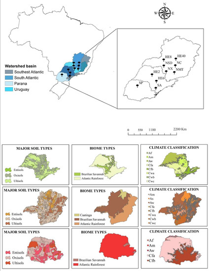
Figure 1.
Geographical distribution of the datasets and climatic properties of the studied sites.
The selected regions have different soils, vegetation types, biomes, and climate characteristics. Most of the study areas are covered by Oxisols, Ultisols, and Entisols. The biomes covered by this study are Brazilian Savannah (Cerrado) and the Atlantic Rainforest (Mata Atlântica), two of the three larges biomes in Brazil. Brazil has three climate types according to Köppen-Geiger climate classification [43]: Tropical Zone—A (81.4%), Dry Zone—B (4.9%) and Humid Subtropical Zone—C (13.7%). The sites applied in this study are described within the 8 following subtypes: Af (without dry season), Am (monsoon), Aw (with dry winter), As (with dry summer), Cfa (oceanic climate without dry season and with hot summer), Cfb (oceanic climate without dry season and with temperate summer), Cwa (with dry winter and hot summer), and Cwb (with dry winter and temperate summer).
2.2. Database Structure
The structure of the database studied in the nonlinear fitting algorithm is designed to encompass several forest types and their wide heterogeneity. The goal is to perform a complete and robust experiment to test the hybrid algorithm and its dynamic range approach. To that end, 5834 individual tree observations were selected from 12 sites, where the diameter at breast height (d) (in centimeters, 1.3 m aboveground) and total height (h) (in meters) were measured. The samples were selected from different forest types, classified by Veloso et al. [44] as Brazilian Savannah (Cerradão), Atlantic Rainforest (Mata Atlântica) and Semi-Deciduous Seasonal Forest (Floresta Estacional Semi-decidual). In addition, commercial fast growth species (Eucalyptus spp. and Pinus spp.) managed under different silvicultural systems were selected: (i) Three datasets composed of 2-, 6-, and 8-year-old planted Eucalyptus spp. stands with a planting density 2 × 2 m in a management system designed for energy wood, pulpwood, and saw timber, respectively, as well as a fourth dataset comprising a 40-year-old planted Eucalyptus spp. stand (2 × 2 m) that had never been harvested nor thinned; and (ii) two datasets composed of 5- and 7-year-old planted Pinus spp. stands with a planting density of 2.2 × 2.2 m that had never been thinned and a dataset comprising an 8-year-old Pinus spp. stand planted with a density of 2.2 × 2.2 m that had been recently thinned at 8 years of age. These regimes are often planted by pulp, fiberboard, and lumber industries in Brazil. Finally, two Brazilian native species were selected that exhibit monodominance behavior (Araucaria augustifolia (Bertol.) and Xylopia brasiliensis Spreng.) and are important for ecological, financial, cultural, and social values.
The database applied in this study presented dispersion and position measures varying within a wide range due to its diverse origins and treatments (Table 1).
The characteristic dispersion and nonlinear correlation within each dataset are shown in Figure 2. The high inner variation must be assigned to the natural and older stands, which present overstock (HE40) and different species (NC, NMT, and NSD). However, some other datasets show less variance within their observations (HE2, HE6, HE8, NX, SA, SP5, and SP8), which could lead to a requirement of less computational effort to adjust a model. These datasets come mainly from monocultures. Spearman’s rank correlation (π) (Figure 2) shows a strong relationship between d and h variables (π ≥ 0.7) for most of the dataset. Only in NC and NMT was the correlation not considered to be strong because their origin was from mixed-species natural stands.
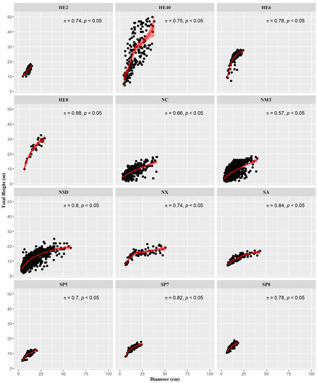
Figure 2.
Scatter plot of total height as a function of diameter for each dataset, illustrating the Spearman’s correlation coefficient and associated p-value (p).
2.3. Fitting Approach
2.3.1. Nonlinear Regression Models
Twelve nonlinear biological growth models (Table 2) were chosen to test the robustness of the hybrid method. These type of models have been frequently applied to predict variables in forest science, e.g., total tree height [45,46,47], dominant tree height [48], and individual tree variables [49].
The prediction of the total height (h) is widely applied in forestry studies, usually presenting sufficient correlation with diameter at breast height (d) to perform regression analysis. The hypsometric patterns tend to exhibit nonlinear behavior, whereas the linear h(d) equations may only be applicable to tested tree sizes and standard conditions [50]. Owing to the widespread use of the h(d) relationship in forest management and the complexity of its fitting and estimating features, it was used to test the novel algorithm. Therefore, twelve nonlinear regression models were selected from the forest science literature and used to estimate the total height (h) as a function of diameter at breast height (d) (Table 2).
Table 2.
Nonlinear regression models selected to test the hybrid algorithm with dynamic range.
Table 2.
Nonlinear regression models selected to test the hybrid algorithm with dynamic range.
| Parameter | ID | Model Reference | Model |
|---|---|---|---|
| 2 | 1 | Meyer 1 | |
| 2 | Burkhart 2 | ||
| 3 | 3 | Monomolecular 1 | |
| 4 | Mitcherlich 1 | ||
| 5 | Gompertz 1 | ||
| 6 | Logistic 3 | ||
| 7 | Chapman-Richards 4 | ||
| 8 | Bailey 2 | ||
| 4 | 9 | Von Bertalanffy 1 | |
| 10 | Bailey 2 | ||
| 11 | Zeide 2 | ||
| 12 | Richards 2 |
Notes: h(d)—total tree height as a function of diameter at breast height (d); b1—asymptote parameter; b2—curve slope parameter; b3—rate to reach the asymptote parameter; b4—allometric constant parameter; ε—random error; exp—mathematical exponential expression. 1—[29]; 2—[3]; 3—[51]; 4—[52].
2.3.2. Hybrid Method
In this section, we describe the proposed hybrid method to fit nonlinear regression models without knowledge of the initial parameter values. The method has two stages: (a) the genetic-dynamic approach, i.e., the genetic algorithm developed to predict the initial parameter values, and (b) the statistical approach, i.e., model fitting by applying a widely applied statistical nonlinear regression algorithm (Levenberg–Marquardt). We named the proposed hybrid approach GALM (genetic algorithm + Levenberg–Marquardt).
The main procedure of the hybrid algorithm is illustrated flow chart in Figure 3. It covers both stages, i.e., the GA procedures and the classic regression method.
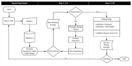
Figure 3.
Hybrid algorithm processing scheme.
The hybrid algorithm implementation was developed using R software (Version 4.2.1) [53]. In the first step, we coded and designed a genetic algorithm (GA) with a modification in the fitting strategy to encompass a dynamic shrinking characteristic, and in the second step, we applied the R package (Version 1.2-2) minpack.lm [54] to fit the nonlinear regression models by the Levenberg–Marquardt method for all databases following 100 repetitions. All computational tests were performed on a Desktop/Intel® Core™ i5-3570 (3.4 GHz).
- Step 1: Genetic Dynamic Approach
In order to control the genetic algorithm convergence, previous tests were applied. As an evolving population algorithm, the GA requires predefinitions to start off its iterations. The initial conditions for the GA are described in this paper as the population size, fitness function, and genetic operators (selection, crossover, and mutation operators). The population size is represented by a group of individuals, which, in the context of this study, are the estimated value of the parameters to be evaluated at every iteration, i.e., the potential squared error of the equation. The genetic operators play an enhancing role through the iterations, approximating the curve within the dataset. In this study, in order to provide wider search of the solution, owing to the lack of previous information about the initial parameter estimate, we set a maximum population size of 300 individuals and 100 iterations as the stop criteria, define as k iterations, where k ∈ {1, …, 100}. The fitness function (Q) minimizes the residual sum of squares (Equation (1)), where h is the vector of the observed total height in meters, is the estimated vector of parameters for iteration k considering the models in Table 1, and X is the design matrix.
The parameters are obtained from a random generation structure within a predefined symmetric interval (R = [−r, +r]), such that R~Uniform (−r, +r), in which all values have the same probability of being selected. Thus, the range (R) has an expected value and variance of E[R] = 0 and V[R] = r2/3, respectively, as the parameters of the uniform distribution were set to be symmetric. Therefore, the underlying objective function is to minimize the variance of the model predictions by shrinking the value of r toward zero; consequently, the estimated parameters will have the same pattern. This strategy improves the minimization strategy for the overall variance of the parameters obtained by the GA procedure through the genetic operators, also improving the efficiency of the genetic selection operator and providing shrinking characteristics to the estimated parameters () by considering a limiting factor as a set operator, i.e., min {,…,} for iteration k.
Initially, a high value is assigned for r (|r| = 100) to account for the lack of previous information about the data and the model, which implies that all parameters start the process with a random value obtained from the same range and distribution (R~Uniform (−r, +r)). This initial interval R tends to decrease according to the iterations through the dynamic strategy as the fitness function is improved. The pseudocode of the dynamic range is given in Table 3.
Table 3.
Pseudocode for the dynamic range strategy implementation.
where the function gk represents the best candidate solution in iteration k, and the function g* is the best solution found until iteration k. The dynamic range function provides adaptation in order to accelerate the convergence of the parameters to the local optima. Thus, the range interval changes according to the current best solution, but the interval remains untouched if the randomness seed of the searching phase of the algorithm reaches a place in the solution space that is not considered a source of good estimates based on the fitness function. After execution of the dynamic range strategy, the genetic operators are activated.
- (1)
- Selection Operator: This operator plays the role of the most adapted individual selector, similar to Darwin’s theory of biological selection, which asserts that the most adapted individual has the greatest probability of survival. Computationally, this is implemented by a random search of the population, creating a new set and selecting individuals according to their fitness values [37]. Tournament selection (Equation (2)) was chosen to control the diversity losses [38], selecting two individuals (f(x*) and f(y*)) from the pool of parents (population). In order to obtain the most adapted parents, this operator chooses the best value of fitness in every defined pair. Thereafter, the best individuals are selected to crossover proceedings.
f(z*) = min{f(z1), f(z2), …, f(z300)}
- (2)
- Crossover Operator: This is an important operator of the GA, providing the exploitation phase of the solution search [55]. Similar to biology, the crossover is responsible for exchanging genes from parents to their offspring, producing phenotypic variability, i.e., a combination of parameter estimates from selected parents with the aim of producing offspring containing characteristics of both best selected individuals in the selection operator. The crossover operator has one swapping gene for each selected pair of parents (Figure 4).
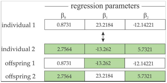 Figure 4. One-gene swapping strategy for a two-parameter model.
- (3)
- Mutation Operator: According to [55], mutation performs solution exploration, increasing the diversity of the population. This operator imitates biological mutation as described in Darwin’s theory, which says that there are some “random changes” in an individual’s characteristics that if these changes are skill-increasing, they will be passed from parents to offspring, maintaining differences from the other individuals (diversity). Mutation maintains genetic population diversity and provides an escape mechanism from a local optima space [28]. Computationally, mutation works by randomly selecting a parameter and a new value for this parameter according to the interval R described above. We applied a 60% random mutation rate for each iteration. We chose a high mutation rate for this study to account for the lack of previous information about the datasets and the mathematical properties of the loss function (nonlinear models).
- Step 2: Statistical Approach
The second strategy of the hybrid algorithm is associated with a classic nonlinear regression solving algorithm, the Levenberg–Marquardt Method (LM). The parameter values derived from the best output from the GA convergence were applied in this stage as preoptimized initial guesses. Considering the dataset (xi, yi) to be fitted, where xi is the independent and yi is the dependent variable; i = 1, …, n, where n is the number of observations, βp is the vector of parameters; and p = 1, …, P, where P is the number of parameters.
The LM algorithm was first idealized in [56], named Levenberg’s method, considering Newton’s method in its update function. Newton’s method is a widely studied and applied algorithm for nonlinear optimization and uses Taylor series for approximation of the nonlinear function to iteratively improve an initial vector of parameters (β0) for β, where β is a vector of parameters that minimizes the residual sum of squares and keeps improving the estimates until there is no change [57]. An improvement of Levenberg’s method proposed in [58] incorporated the estimated local curvature information into the original Newton’s update function. The Levenberg–Marquardt algorithm was implemented as a robust technique by Moré [59], who approached the step-bound Δ, which updates its choice depending on the ratio (ρ(β)) between the actual reduction and the prediction reduction. This ratio is obtained by decomposition in the linear system by measuring the agreement between the linear and the nonlinear function [60]. This step-bound concept is a prior attempt of trust-region approach, using ρ(β) to choose Δ, as expressed in Equation (3).
To update Δ, Equation (3) must be kept at a reasonable value such that if ρ(β) ≥ ¾, then Δ increases, whereas if ρ(β) ≤ ¼, then Δ must be decreased. For more specific rules for updating Δ, see [60]. The author still states that α > 0 is the Levenberg–Marquardt parameter if |F(α)| ≤ σΔ, where σ ∈ (0,1) specifies the relative error in , where D is a diagonal matrix that takes into account the scale of the problem, i.e., the database module [60].
2.4. Assessment of the Hybrid Approach
We selected 12 models with nonlinear functions with biological interpretation of parameters from the literature with varying numbers of parameters to be estimated (2, 3, and 4 parameters) and varied mathematical structure. A combinatorial problem arises when every model is matched with 12 databases. The procedure runs 100 times to validate the results due to the stochastic seed of GA (Step 1). Therefore, the experimental repetitions reached 14,400 (12 × 12 × 100) runs when combined with the nonlinear regression method (Step 2) assigned to the GA approach (the hybrid GALM). The statistical criteria derived from the error were applied to evaluate the consistency of the parameters displayed by the hybrid approach: MAE, mean absolute error (4); , adjusted coefficient of determination (5); Bias (6); and RMSE, root mean square error (7).
where represents the observed total height of individual tree i, is the estimated total height for tree i, n represents the sample size, p is the number of parameters of the target model, and is the uncorrected coefficient of determination given by 1—SSE/SST, where SSE is the sum of squares error and SST is the corrected sum of squares total.
3. Results
3.1. Hybrid Modeling Assessment
3.1.1. Genetic Algorithm Approach
The designed GA was able to predict the initial parameters for all tested models and datasets in which the fitness function decreased throughout the iterations by model parameter classes 2pg, 3pg, and 4pg, which refer to models with two, three, and four parameters, respectively (Figure 5). The GA improved the initial population using a randomized procedure. This was attributed to the genetic algorithm intrinsic factors, including mutation rate, population size, and the dynamic range approach. However, the four-parameter models (4pg) were more complex in minimizing the error function due to their higher degree of nonlinearity (Figure 5, A-4pg). Models with a complex structure tend to not converge easily depending on the initial guess required by the nonlinear optimization algorithms. However, the GA provided reliable initial guesses, which contributed to the success of all GALM conversions.
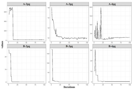
Figure 5.
Logarithm of best average error (set A) and change in dynamic range (set B) by parameter class (2pg—models with two parameters; 3pg—models with three parameters; and 4pg—models with four parameters).
The change in the dynamic range (Figure 5, set B) in each parameter class provides an approximation of the efficiency of the fitting process, in which the dynamic range strategy plays an important role. The logarithm of best average error (Figure 5, set A) presents an abrupt reduction (A-2pg and A-4pg) (Figure 5), which can be associated with a slight change in the dynamic range presented in B-2pg and B-4pg. After small changes in the search range, the error exhibited stabilization for A-2pg and small oscillations for A-4pg (Figure 5). For the latter case, GA found the best error possible and stabilized the dynamic range (Figure 5, B–4pg) to refine the search around iteration 26. Solutions less optimal than those found by GA for the A-4pg (Figure 5) were activated after iteration 26, and although the error increased, the dynamic range remained stable, showing consistency across iterations. The changes in the error for this case may be related to the GA steps, as the dynamic range was kept stable.
For the 3pg parameter class (sets A and B in Figure 5), an inverse pattern was observed, such that a large and abrupt change in the dynamic range (Figure 5, B-3pg) had no significant effect on the error, reducing from 16 to around 10 (Figure 5, A-3pg). For this case, the dynamic range selected high initial values according to its characteristics of equal probability of obtaining the values within the initial range. Owing to the small reduction in the error, the dynamic range rapidly adapted to the new best solution and stabilized after a few subsequent iterations. This is an expected feature, owing to the broader initial range for all parameter class models to account for the lack of information about the datasets and the initial guesses. If the initial guesses were provided with a priori information, then the expected behavior of the changes in the dynamic range should resemble that expressed in B-2pg and B-4pg (Figure 5)—perhaps even more stable than the displayed changes.
The dynamic range strategy was essential to provide the GA better coverage of the solution space and more tools to avoid the local optima spots, which are usually difficult to detect, requiring significant efforts for any non-deterministic method. The parameter range interval changes when the algorithm finds a better solution, supporting the stochastic pattern to improve the population average error. A robust convergence algorithm combined with a short run time is desired to determine the initial parameters. This problem can be solved in a straightforward manner using GA associated with the dynamic range approach.
3.1.2. Hybrid Approach
The GALM algorithm spent an average of 22.16 s, with a minimum of 1.0 and a maximum of 58.56 s, to fit all models within all databases, achieving total fitting success, regardless of database variability and the complexity of the mathematical model. Although the processing time depends on the size of the applied dataset, the GALM achieved a fast convergence time, despite no previous acknowledge of the database.
The error statistics showed equality in fitting among all models within the databases and experimental repetitions (Table 4).
Table 4.
Average error statistics, with standard deviation in parenthesis (both in meters) for GALM, considering all tested nonlinear regression models and databases for hypsometric relationships.
The hybrid method estimates the parameters for all models and databases without returning any non-convergence output. In most tests, the parameter variation is either very low or inexistent. Figure 6 shows a box plot of all 100 repetitions performed by the algorithm on the Burkhart model estimates. The estimates are stables for almost all databases, presenting 0.1% variation in NC for parameter b2 and NSD for parameter b1.
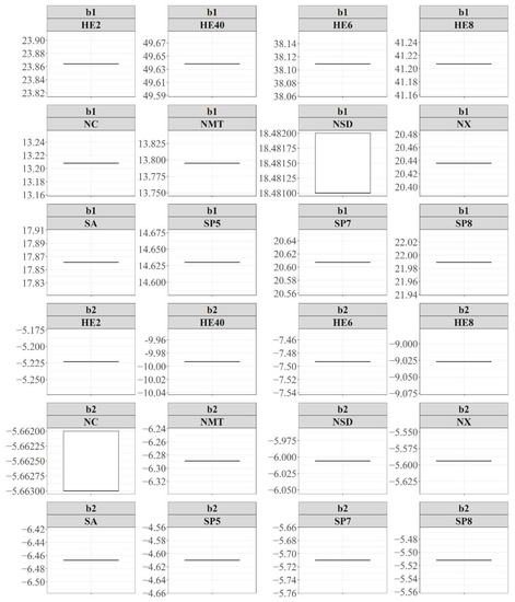
Figure 6.
Dispersion box plot of GALM estimate parameters with 100 repetitions.
4. Discussion
A complex database encompassing by 12 silviculture prescriptions and species was used to fit the hypsometric relationship on 12 nonlinear regression models with biological interpretation. The hybrid method has two stages: (1) the genetic-dynamic-approach, providing high-quality initial parameter estimates; and (2) the Levenberg–Marquardt method, using the initial parameter estimates from Stage 1 to estimate the final set of parameter estimates.
The number of parameters within a model is an underlying reason for the increased complexity of the parameter estimate analyses. We addressed this complexity by comparing the high computational effort required to execute GALM to fit the models with four parameters (Figure 5, A-4pg). However, the dynamic range strategy showed the same pattern for all groups of models by reducing the parameter interval from a high value to a reasonable range before 25 iterations in the first stage (Figure 5, B-4pg). In Ref. [24], random effect parameters applied to the segmented taper model presented in [25] could not be adjusted for combinations of fixed and random effects, which is common in mixed effect regression. The authors derived algebraic constraints in the taper equation, which may have caused convergence failure. Non-convergence is likely to occur when changes in the mathematical structure of the model are taken into consideration and the initial seeds are not updated accordingly. The first derivative of the model usually helps in the fitting process, although in several examples, non-convergence persists due to the high sensitivity of the classical methods to the initial seeds. A hybrid approach with metaheuristic optimization of prior assumptions about the initial guesses is recommended. In Ref. [15], the authors listed several nonlinear models often applied in biological sciences and provided information about tools for fitting many of them. The authors stated that some transformations should be applied in order to avoid changes in the initial intrinsic characteristics of these models, as they are based on nonlinear model families, such as Gompertz, exponential, monomolecular, and logistic models. In the GALM context, neither the mathematical structure of the model nor number of parameters had a significant influence on the convergence process, as the hybrid approach reached 100% convergence in all tested cases, owing to its main advantage of application the genetic algorithm as the initial seed provider. In addition, dynamic range modification improves the variance of the estimates, and the enhancement phase (Step 2) results in more specific evaluation of the space of solutions than would be achieved if only the standard configuration of GA were applied. Whereas the genetic operators execute the local search and scape from local optima, the dynamic range forces the shrinkage of the space of solutions, providing more efficient solution exploitation. Therefore, GALM could be helpful for improving the calibration rate in mixed effect nonlinear studies, such as in [24,61,62], as the random effect would be identified as an additional parameter with constraints with respect to the initial seed estimate, considering the mathematical structure of a specific model and the dataset characteristics.
In Ref. [63], the authors applied simulations to ensure the reliability and accuracy of a modified maximum likelihood procedure. In the GALM approach, the simulations produced concrete results (Figure 6 and Table 4), demonstrating the estimation capacity of the hybrid algorithm in producing stable and reliable parameter estimates, although with a highly variable dataset (Figure 2). Stage 2 ensures that the stability of the hybrid method is maintained if the provided initial solution is accurate toward the optima. The estimated parameter variation (Figure 6) demonstrates that the association of GA with LM provides more intuitive and direct analysis in the nonlinear modeling context. Table 4 presents the evaluation metrics for each model; regardless of the number of parameters and mathematical structure, the statistic metrics of the hypsometric relationship were similar (MAE, Bias, RMSE, and ), with a coefficient of variation for each metric across the models of 0.56%, 8.45%, 0.58%, and 0.68%, respectively. The stochastic outcomes under uncertainties from GA resulted in a robust and efficient way to estimate the parameters, also reported in [37,38].
A high stability of GALM estimates was achieved for all databases, except for NSD parameter b1 and NC parameter b2 (Figure 6). In these two cases, the datasets are composed of a stand of natural mixed species with no stratification, which can lead to a diffuse pattern due to high biological variation among species. The variations in parameter b1 and b2 indicate that these parameters present higher uncertainty compared to the other parameters of the Burkhart model displayed in Figure 6. A sensitivity analysis might be necessary to reduce the variation in these estimates. Studies considering sensitivity analysis of parameter estimation are common in forestry, for example, in [61], the authors investigated forest growth variables by introducing a modification of the Taylor approximation series to fit mixed multilevel nonlinear models. They were not able to achieve convergence by applying mixed effects in all parameters of a version of the Chapman–Richards function; instead, they applied it to the slope parameter only. In order to obtain the initial solutions for that combination, the authors applied several repetitive steps when fitting the Chapman–Richards function for each plot separately, then regressed each plot-specific parameter estimate over the covariate trees per hectare. The GALM executes the second phase proposed in [61] using the Levenberg–Marquardt algorithm, which also uses Taylor approximation in the update function and introduces the concept of a trust region [60], achieving total adjustment with less effort and more time efficiency, with a maximum computational time of 58.56 with 14,400 repetitions without prior knowledge about the database or model mathematical structure. Furthermore, the shrinking characteristic applied to the parameter estimates based on the dynamic range strategy provides less variation in the model predictions, which makes the biological characteristics of the nonlinear parameters a matter of interpretation according to their scale.
There are few desired characteristics in the development of a new parameter optimization method, including low processing time, high-quality initial solutions, reliability, and stability of the final solution. The GALM presents conclusive metrics toward these objectives, corroborating the results of similar studies [64,65]. The use of metaheuristics as a nonlinear adjustment method has been applied in some studies with similar results as those reported in the present study. In Ref. [28], the authors proposed a method to change the parameter domain using several genetic algorithms, known a ADM—conceptually similar to our proposed approach. They changed the likelihood function to search for a new parameter domain. A similar strategy was applied in the dynamic range calculation, for which parameter range adaptation was updated after every best loss function was found throughout Step 2 processing. In Ref. [66], the authors minimized the model calibration complexity using a modified scatter search algorithm, achieving efficiency in reaching the global optima. In Ref. [67], the authors applied a combined strategy to model a system of biodiesel production using a backpropagation fuzzy rule-based model to provide coefficients of an optimization model that updates the goals of production for the fitting phase. In Ref. [68], the authors proposed the use of GA for two purposes—feature selection and fitting strategy—without using classical methods to estimate the parameters. Although the performance of parameter estimates was not validated, the authors highlighted the advantage of using GA for both feature selection and parameter estimation in nonlinear regression, as no prior information about the initial guesses is required. In the abovementioned studies, the authors attempted to facilitate the fitting process through different approaches, reinforcing the necessity of more efficient methods. In some cases, this represents a significant increase in complexity for the fitting method, which translates into difficulties with respect to replication. With the GALM approach, we present a straightforward strategy to improve the gains in the GA phase by simply reducing the estimates toward the origin as the solutions are improved through Step 1. The pseudocode presented in Table 3 exemplifies the implementation of our strategy. This dynamic range update approach provides search efficiency for improved solutions with no previous knowledge about the dataset or the model structure, reducing the complexity of calibration in nonlinear models and combining the strengths of widely applied optimization methods. In essence, the GALM is a modified backpropagation strategy. In Stage 1, i.e., the dynamic range update, the quality of further solutions depends on previous solutions in a connected flow of improvement. When Stage 2 begins, the solutions are already close to optimal; therefore, fitting success is achieved with no extra effort.
The GALM approach presented here highlights some of the main difficulties associated with biological nonlinear analyses, i.e., the attainment of the initial set of values for the fitting model and, consequently, failure in accurate estimation of the model parameters. The hybrid method overcomes the drawbacks of nonlinear biological analysis of a lack of prior information about the dataset and biological interpretation of the parameters.
5. Conclusions
In this study, we investigated the use of a hybrid method based on the association of the strengths of a genetic algorithm and the Levenberg–Marquardt method in order to improve the capacity of fitting nonlinear models with biological interpretation of hypsometric relationships. We estimated the parameters of nonlinear regression models with biological interpretation without prior information about the dataset or the mathematical structure of the nonlinear models. The overall result shows that this association can be used to improve the calibration of parameters and the frequency of successes in fitting a nonlinear model in forest modeling studies, particularly for hypsometric relationships, which can pose challenges in obtaining parameter estimates, owing to its degenerated characteristic. The presented hybrid method overcomes this issue, providing estimates for all tested datasets, regardless of complexity.
The dynamic range strategy improves the search space and reduces the variance of the parameters by shrinking them toward smaller values. This strategy assists the genetic operators by making the search space more specific, improving the set of solutions.
The combination of GM with the LM method integrates the trust region concept embedded in this method. The proposed GALM approach provides reliable estimates and is therefore recommended for nonlinear studies applied in forestry, specifically for parameters of biological interpretation.
Author Contributions
C.A.U.M.: conceptualization, investigation, methodology, software, data curation, formal analysis, and writing—original draft preparation; R.M.O.: investigation, methodology, and writing—review and editing; J.P.R.: writing—review and editing; H.F.S.: data curation, validation, and writing—review and editing; L.R.G.: conceptualization, supervision, methodology, funding acquisition, project administration, and writing—reviewing and editing. All authors have read and agreed to the published version of the manuscript.
Funding
This research received no external funding.
Data Availability Statement
Data generated or analyzed during this study are not available due to legal restrictions.
Acknowledgments
The authors would like to thank the Postgraduate Program in Forest Engineering, Federal University of Lavras (Brazil), for the opportunity to develop this study.
Conflicts of Interest
The authors declare no conflict of interest. The funders had no role in the design of the study; in the collection, analyses, or interpretation of data; in the writing of the manuscript; or in the decision to publish the results.
References
- Fischer, C.; Schönfelder, E. A Modified Growth Function with Interpretable Parameters Applied to the Age–Height Relationship of Individual Trees. Can. J. For. Res. 2017, 47, 166–173. [Google Scholar] [CrossRef]
- Huang, S.; Titus, S.J.; Wiens, D.P. Comparison of Nonlinear Height–Diameter Functions for Major Alberta Tree Species. Can. J. For. Res. 1992, 22, 1297–1304. [Google Scholar] [CrossRef]
- Fang, Z.; Bailey, R.L. Height-Diameter Models for Tropical Forests on Hainan Island in Southern China. For. Ecol. Manag. 1998, 110, 315–327. [Google Scholar] [CrossRef]
- Mehtätalo, L.; de-Miguel, S.; Gregoire, T.G. Modeling Height-Diameter Curves for Prediction. Can. J. For. Res. 2015, 45, 826–837. [Google Scholar] [CrossRef]
- Fu, L.; Sun, H.; Sharma, R.P.; Lei, Y.; Zhang, H.; Tang, S. Nonlinear Mixed-Effects Crown Width Models for Individual Trees of Chinese Fir (Cunninghamia Lanceolata) in South-Central China. For. Ecol. Manag. 2013, 302, 210–220. [Google Scholar] [CrossRef]
- Fu, L.; Sharma, R.P.; Hao, K.; Tang, S. A Generalized Interregional Nonlinear Mixed-Effects Crown Width Model for Prince Rupprecht Larch in Northern China. For. Ecol. Manag. 2017, 389, 364–373. [Google Scholar] [CrossRef]
- Bianchi, S.; Hale, S.; Cahalan, C.; Arcangeli, C.; Gibbons, J. Light-Growth Responses of Sitka Spruce, Douglas Fir and Western Hemlock Regeneration under Continuous Cover Forestry. For. Ecol. Manag. 2018, 422, 241–252. [Google Scholar] [CrossRef]
- Rayner, M.E. Evaluation of Six Site Classifications for Modelling Timber Yield of Regrowth Karri (Eucalyptus Diversicolor F. Muell.). For. Ecol. Manag. 1992, 54, 315–336. [Google Scholar] [CrossRef]
- Fontes, L. Modelling Dominant Height Growth of Douglas-Fir (Pseudotsuga Menziesii (Mirb.) Franco) in Portugal. Forestry 2003, 76, 509–523. [Google Scholar] [CrossRef]
- Lekwadi, S.O.; Nemesova, A.; Lynch, T.; Phillips, H.; Hunter, A.; Mac Siúrtáin, M. Site Classification and Growth Models for Sitka Spruce Plantations in Ireland. For. Ecol. Manag. 2012, 283, 56–65. [Google Scholar] [CrossRef]
- Shvets, V.; Zeide, B. Investigating Parameters of Growth Equations. Can. J. For. Res. 1996, 26, 1980–1990. [Google Scholar] [CrossRef]
- Mønness, E. The Power-Normal Distribution: Application to Forest Stands. Can. J. For. Res. 2011, 41, 707–714. [Google Scholar] [CrossRef]
- Graybill, F.A.; Iyer, H.K. Regression Analysis: Concepts and Applications; Duxbury Press: London, UK, 1994. [Google Scholar]
- Pienaar, L.V.; Turnbull, K.J. The Chapman-Richards Generalization of Von Bertalanffy’s Growth Model for Basal Area Growth and Yield in Even-Aged Stands. For. Sci. 1973, 19, 2–22. [Google Scholar]
- Paine, C.E.T.; Marthews, T.R.; Vogt, D.R.; Purves, D.; Rees, M.; Hector, A.; Turnbull, L.A. How to Fit Nonlinear Plant Growth Models and Calculate Growth Rates: An Update for Ecologists. Methods Ecol. Evol. 2012, 3, 245–256. [Google Scholar] [CrossRef]
- Tashkova, K.; Šilc, J.; Atanasova, N.; Džeroski, S. Parameter Estimation in a Nonlinear Dynamic Model of an Aquatic Ecosystem with Meta-Heuristic Optimization. Ecol. Modell. 2012, 226, 36–61. [Google Scholar] [CrossRef]
- Pedersen, M.W.; Berg, C.W.; Thygesen, U.H.; Nielsen, A.; Madsen, H. Estimation Methods for Nonlinear State-Space Models in Ecology. Ecol. Modell. 2011, 222, 1394–1400. [Google Scholar] [CrossRef]
- Payandeh, B. Some Applications of Nonlinear Regression Models in Forestry Research. For. Chron. 1983, 59, 244–248. [Google Scholar] [CrossRef]
- Khan, D.M.; Ihtesham, S.; Ali, A.; Khalil, U.; Khan, S.A.; Manzoor, S. An efficient and high breakdown estimation procedure for nonlinear regression models. Pak. J. Stat. 2017, 33, 223–236. [Google Scholar]
- Ratkowsky, D.A. Principles of Nonlinear Regression Modeling. J. Ind. Microbiol. 1993, 12, 195–199. [Google Scholar] [CrossRef]
- Draper, N.R.; Smith, H. Applied Regression Analysis; John Wiley & Sons: New York, NY, USA, 1998; p. 326. [Google Scholar]
- Wright, S.; Nocedal, J. Numerical Optimization; Springer: Berlin/Heidelberg, Germany, 1999; Volume 35, p. 7. [Google Scholar]
- Parresol, B.R. Additivity of Nonlinear Biomass Equations. Can. J. For. Res. 2001, 31, 865–878. [Google Scholar] [CrossRef]
- Cao, Q.V.; Wang, J. Calibrating Fixed- and Mixed-Effects Taper Equations. For. Ecol. Manag. 2011, 262, 671–673. [Google Scholar] [CrossRef]
- Max, T.A.; Burkhart, H.E. Segmented Polynomial Regression Applied to Taper Equations. For. Sci. 1976, 22, 283–289. [Google Scholar]
- Chumney, E.C.G.; Simpson, K.N. Methods and Designs for Outcomes Research; ASHP: Bethesda, MD, USA, 2006. [Google Scholar]
- Holmström, K.; Petersson, J. A Review of the Parameter Estimation Problem of Fitting Positive Exponential Sums to Empirical Data. Appl. Math. Comput. 2002, 126, 31–61. [Google Scholar] [CrossRef]
- Tomioka, S.; Nisiyama, S.; Enoto, T. Nonlinear Least Square Regression by Adaptive Domain Method with Multiple Genetic Algorithms. IEEE Trans. Evol. Comput. 2007, 11, 1–16. [Google Scholar] [CrossRef]
- Fekedulegn, D.; Mac Siurtain, M.P.; Colbert, J.J. Parameter Estimation of Nonlinear Growth Models in Forestry. Silva Fenn. 1999, 33, 327–336. [Google Scholar] [CrossRef]
- Křivý, I.; Tvrdík, J. The Controlled Random Search Algorithm in Optimizing Regression Models. Comput. Stat. Data Anal. 1995, 20, 229–234. [Google Scholar] [CrossRef]
- Tang, K.; Li, T. Comparison of Different Partial Least-Squares Methods in Quantitative Structure—Activity Relationships. Anal. Chim. Acta 2003, 476, 85–92. [Google Scholar] [CrossRef]
- Imbault, F.; Lebart, K. A Stochastic Optimization Approach for Parameter Tuning of Support Vector Machines. In Proceedings of the 17th International Conference on Pattern Recognition, Cambridge, UK, 26 August 2004; Volume 4, pp. 597–600. [Google Scholar] [CrossRef]
- Pouzol, T.; Kopf, C.; Lévi, Y.; Bertrand-Krajewski, J.-L. Stochastic Modelling of Pharmaceuticals Path from Sales and Deliveries to Wastewater Treatment Plant at Hourly Scale. Proc. SPN 2016, v. 8, 264–265. [Google Scholar]
- Leehter, Y.; Sethares, W.A. Nonlinear Parameter Estimation via the Genetic Algorithm. IEEE Trans. Signal Process. 1994, 42, 927–935. [Google Scholar] [CrossRef]
- Chatterjee, S.; Laudato, M.; Lynch, L.A. Genetic Algorithms and Their Statistical Applications: An Introduction. Comput. Stat. Data Anal. 1996, 22, 633–651. [Google Scholar] [CrossRef]
- Karr, C.L.; Weck, B.; Freeman, L.M. Solutions to Systems of Nonlinear Equations via a Genetic Algorithm. Eng. Appl. Artif. Intell. 1998, 11, 369–375. [Google Scholar] [CrossRef]
- Kapanoglu, M.; Koc, I.O.; Erdogmus, S. Genetic Algorithms in Parameter Estimation for Nonlinear Regression Models: An Experimental Approach. J. Stat. Comput. Simul. 2007, 77, 851–867. [Google Scholar] [CrossRef]
- Jin, Y.-F.; Yin, Z.-Y.; Shen, S.-L.; Hicher, P.-Y. Selection of Sand Models and Identification of Parameters Using an Enhanced Genetic Algorithm. Int. J. Numer. Anal. Methods Geomech. 2016, 40, 1219–1240. [Google Scholar] [CrossRef]
- Moin, N.H.; Salhi, S.; Aziz, N.A.B. An Efficient Hybrid Genetic Algorithm for the Multi-Product Multi-Period Inventory Routing Problem. Int. J. Prod. Econ. 2011, 133, 334–343. [Google Scholar] [CrossRef]
- Li, T.-H.; Lucasius, C.B.; Kateman, G. Optimization of Calibration Data with the Dynamic Genetic Algorithm. Anal. Chim. Acta 1992, 268, 123–134. [Google Scholar] [CrossRef]
- Haj Seyed Hadi, M.R.; Gonzalez-Andujar, J.L. Comparison of Fitting Weed Seedling Emergence Models with Nonlinear Regression and Genetic Algorithm. Comput. Electron. Agric. 2009, 65, 19–25. [Google Scholar] [CrossRef]
- Forrest, S. Genetic Algorithms: Principles of Natural Selection Applied to Computation. Science 1993, 261, 872–878. [Google Scholar] [CrossRef]
- Alvares, C.A.; Stape, J.L.; Sentelhas, P.C.; De Moraes Gonçalves, J.L.; Sparovek, G. Köppen’s Climate Classification Map for Brazil. Meteorol. Z. 2013, 22, 711–728. [Google Scholar] [CrossRef]
- Veloso, H.P.; Rangel-Filho, A.L.R.; Lima, J.C.A. Classificação Da Vegetação Brasileira, Adaptada a Um Sistema Universal; Ibge—Instituto Brasileiro de Geografia e Estatistica: Rio de Janeiro, Brazil, 1991; ISBN 8524003847.
- Temesgen, H.; Monleon, V.J.; Hann, D.W. Analysis and Comparison of Nonlinear Tree Height Prediction Strategies for Douglas-Fir Forests. Can. J. For. Res. 2008, 38, 553–565. [Google Scholar] [CrossRef]
- Özçelik, R.; Diamantopoulou, M.J.; Crecente-Campo, F.; Eler, U. Estimating Crimean Juniper Tree Height Using Nonlinear Regression and Artificial Neural Network Models. For. Ecol. Manag. 2013, 306, 52–60. [Google Scholar] [CrossRef]
- Misik, T.; Antal, K.; Kárász, I.; Tóthmérész, B. Nonlinear Height-Diameter Models for Three Woody, Understory Species in a Temperate Oak Forest in Hungary. Can. J. For. Res. 2016, 46, 1337–1342. [Google Scholar] [CrossRef]
- Wang, Y.; LeMay, V.M.; Baker, T.G. Modelling and Prediction of Dominant Height and Site Index of Eucalyptus Globulus Plantations Using a Nonlinear Mixed-Effects Model Approach. Can. J. For. Res. 2007, 37, 1390–1403. [Google Scholar] [CrossRef]
- Huang, S.; Titus, S.J. Estimating a System of Nonlinear Simultaneous Individual Tree Models for White Spruce in Boreal Mixed-Species Stands. Can. J. For. Res. 1999, 29, 1805–1811. [Google Scholar] [CrossRef]
- Bi, H.; Fox, J.C.; Li, Y.; Lei, Y.; Pang, Y. Evaluation of Nonlinear Equations for Predicting Diameter from Tree Height. Can. J. For. Res. 2012, 42, 789–806. [Google Scholar] [CrossRef]
- Calegario, N. Modeling Eucalyptus Stand Growth Based on Linear and Nonlinear Mixed-Effects Models; University of Georgia: Athens, GA, USA, 2002. [Google Scholar]
- Zeide, B. Analysis of Growth Equations. For. Sci. 1993, 39, 594–616. [Google Scholar] [CrossRef]
- R Core Team. R: A Language and Environment for Statistical Computing 2022. Available online: https://cran.r-project.org/ (accessed on 20 October 2022).
- Elzhov, T.V.; Mullen, K.M.; Spiess, A.-N.; Bolker, B. Minpack.Lm: R Interface to the Levenberg-Marquardt Nonlinear Least-Squares Algorithm Found in MINPACK, Plus Support for Bounds. 2022. Available online: https://cran.r-project.org/web/packages/minpack.lm/minpack.lm.pdf (accessed on 20 October 2022).
- VanderNoot, T.J.; Abrahams, I. The Use of Genetic Algorithms in the Non-Linear Regression of Immittance Data. J. Electroanal. Chem. 1998, 448, 17–23. [Google Scholar] [CrossRef]
- Levenberg, K. A Method for the Solution of Certain Non-Linear Problems in Least Squares. Q. Appl. Math. 1944, 2, 164–168. [Google Scholar] [CrossRef]
- Bates, D.M.; Watts, D.G. Nonlinear Regression Analysis and Its Applications; John Wiley & Sons: Hoboken, NJ, USA, 1990; Volume 32. [Google Scholar]
- Marquardt, D.W. An Algorithm for Least-Squares Estimation of Nonlinear Parameters. J. Soc. Ind. Appl. Math. 1963, 11, 431–441. [Google Scholar] [CrossRef]
- Moré, J.J. The Levenberg-Marquardt Algorithm: Implementation and Theory. In Numerical Analysis; Springer: Bern, Switzerland, 1978; pp. 105–116. [Google Scholar]
- Moré, J.J.; Sorensen, D.C. Computing a Trust Region Step. SIAM J. Sci. Stat. Comput. 1983, 4, 553–572. [Google Scholar] [CrossRef]
- Hall, D.B.; Bailey, R.L. Modeling and Prediction of Forest Growth Variables Based on Multilevel Nonlinear Mixed Models. For. Sci. 2001, 47, 311–321. [Google Scholar]
- Araújo, L.A.; Oliveira, R.M.; Dobner, M.; Jarochinski e Silva, C.S.; Gomide, L.R. Appropriate Search Techniques to Estimate Weibull Function Parameters in a Pinus Spp. Plantation. J. For. Res. 2021, 32, 2423–2435. [Google Scholar] [CrossRef]
- Cao, Q.; Strub, M. Evaluation of Four Methods to Estimate Parameters of an Annual Tree Survival and Diameter Growth Model. For. Sci. 2008, 54, 617–624. [Google Scholar]
- Schwaab, M.; Biscaia, E.C., Jr.; Monteiro, J.L.; Pinto, J.C. Nonlinear Parameter Estimation through Particle Swarm Optimization. Chem. Eng. Sci. 2008, 63, 1542–1552. [Google Scholar] [CrossRef]
- Özkan, E.; Šmídl, V.; Saha, S.; Lundquist, C.; Gustafsson, F. Marginalized Adaptive Particle Filtering for Nonlinear Models with Unknown Time-Varying Noise Parameters. Automatica 2013, 49, 1566–1575. [Google Scholar] [CrossRef]
- Rodriguez-Fernandez, M.; Egea, J.A.; Banga, J.R. Novel Metaheuristic for Parameter Estimation in Nonlinear Dynamic Biological Systems. BMC Bioinform. 2006, 7, 483. [Google Scholar] [CrossRef] [PubMed]
- Inayat, A.; Nassef, A.M.; Rezk, H.; Sayed, E.T.; Abdelkareem, M.A.; Olabi, A.G. Fuzzy Modeling and Parameters Optimization for the Enhancement of Biodiesel Production from Waste Frying Oil over Montmorillonite Clay K-30. Sci. Total Environ. 2019, 666, 821–827. [Google Scholar] [CrossRef]
- Lacerda, T.H.S.; Miranda, E.N.; E Lopes, I.L.; Fonseca, G.R.; França, L.C. de Jesus França, L.C.; Gomide, L.R. Feature Selection by Genetic Algorithm in Nonlinear Taper Model. Can. J. For. Res. 2022, 52, 769–779. [Google Scholar] [CrossRef]


Publisher’s Note: MDPI stays neutral with regard to jurisdictional claims in published maps and institutional affiliations. |
© 2022 by the authors. Licensee MDPI, Basel, Switzerland. This article is an open access article distributed under the terms and conditions of the Creative Commons Attribution (CC BY) license (https://creativecommons.org/licenses/by/4.0/).