Predicting the Future Age Distribution of Conifer and Broad-Leaved Trees Based on Survival Analysis: A Case Study on Natural Forests in Northern Japan

Abstract

Predicting future stand conditions based on tree age is crucial for natural forest management. The objective of this study was to model and predict the future age distribution of Picea jezoensis, Abies sachalinensis, and broad-leaved trees by assessing the past and current survival trends of preserved stands located at the University of Tokyo Hokkaido Forests (UTHF), Furano, Japan. This study analyzed forest census data of four plots (927 trees) in a preserved permanent area over 30 years (1989–2019). Individual tree-ring data were identified using a resistograph to determine the current tree age of the targeted trees. The predicted age distributions nearly converged to the shape of the survival probability curve. Among the scenario predictions, the multimodal age class distribution of P. jezoensis was predominant among all prediction scenarios. In contrast, the exponential shape of A sachalinensis and the age distribution of broad-leaved trees in the 100% scenario gradually shifted to the multimodal shape at the 50% scenario prediction. The species composition of conifer and broad-leaved trees and their age distribution would reach stable states in the long run by reaching a climax state. Therefore, it is theoretically possible to maintain stands under the pre-climax stage by allowing high growth rates at the stand level. The suggested age class-prediction of living and dead trees can improve the natural forest management of UTHF.

1. Introduction

The structural properties and heterogeneity of forests have become essential factors in forest research and management [1]. Therefore, quantitative descriptions of the characteristics and factors shaping natural forests are required to evaluate the silviculture and management practices that would reflect the structural patterns of typical natural forests [2,3].

In addition, studies on the age structure of a forest population may provide insights into past and present regeneration models [4]. Forest management decisions are based on current and future resource conditions [5]. The age structure of a forest is closely related to its history, because trees are long-living organisms [6]. In the case of forest plantations, regeneration determinations typically depend on silvicultural considerations but will eventually be driven by economic concerns [7]. Moreover, attention should be paid to possible changes in the species proportion and diameter distribution of the remaining forest stands when marking trees for harvesting [8]. Therefore, it is important to predict the age structure of living and dead trees in natural forests based on temporal changes.

In a mature natural forest with an even tree recruitment rate and a consistent or decreasing death rate with age, the tree-age distribution would have a so-called reverse-J shape [2,9,10,11,12]. However, this empirical design is difficult to find, because several factors, both autogenic (differences in seed production, seedling appearance, establishment, and inter-tree competition) and allogenic (natural irregularities and pest outbreaks), affect tree regeneration and survival in forests [13]. Therefore, biotic and abiotic variables can significantly affect tree regeneration, growth, productivity, and mortality [14].

Natural forest management and selection systems have grown in many parts of the world because of their stability in forest stand structures [15]. The Stand-based Silvicultural Management System (SSMS), a special natural forest management system that conducts the single-tree selection of over-matured and defective trees based on natural regenerations, has been implemented since 1958 and has a total area of 22,715 ha [16]. The main silvicultural system of the forest is a single-tree selection, and about 20,000 m³ of trees are harvested annually [17]. In forests with “coniferous selective cutting with poor regeneration” in the UTHF, where we cannot continuously expect sufficient new ingrowth trees, tree-age structure has been hardly examined. Wijenayake and Hiroshima [18] developed maturity-level indicators for conifers and broad-leaved trees based on survival analysis of individual tree populations confined to the current state of the forest. However, these indicators are not sufficient to predict future UTHF scenarios. However, in the natural forests of the UTHF, a simple and practical prediction model based on tree age has not been studied, and data from preserved areas have not been used enough for identification of harvestable trees from major conifers and broad-leaved trees.

This study aimed to predict the age distribution of major conifer and broad-leaved trees by considering temporal changes over the periods. The survival analysis techniques deployed by Wijenayake and Hiroshima [19] can be applied as a foundation for future prediction purposes. Therefore, in this study, future age distributions for the upcoming 100 years were predicted based on past and present states of the forest to identify the living and dead trees of each species over the upcoming periods. The long-term temporal trend of tree population changes based on demographic factors, such as mortality and new ingrowth, was estimated to achieve the objective. Then, the age distribution of living and dead trees of major conifer and broad-leaved tree species was predicted over the long term.

2. Materials and Methods

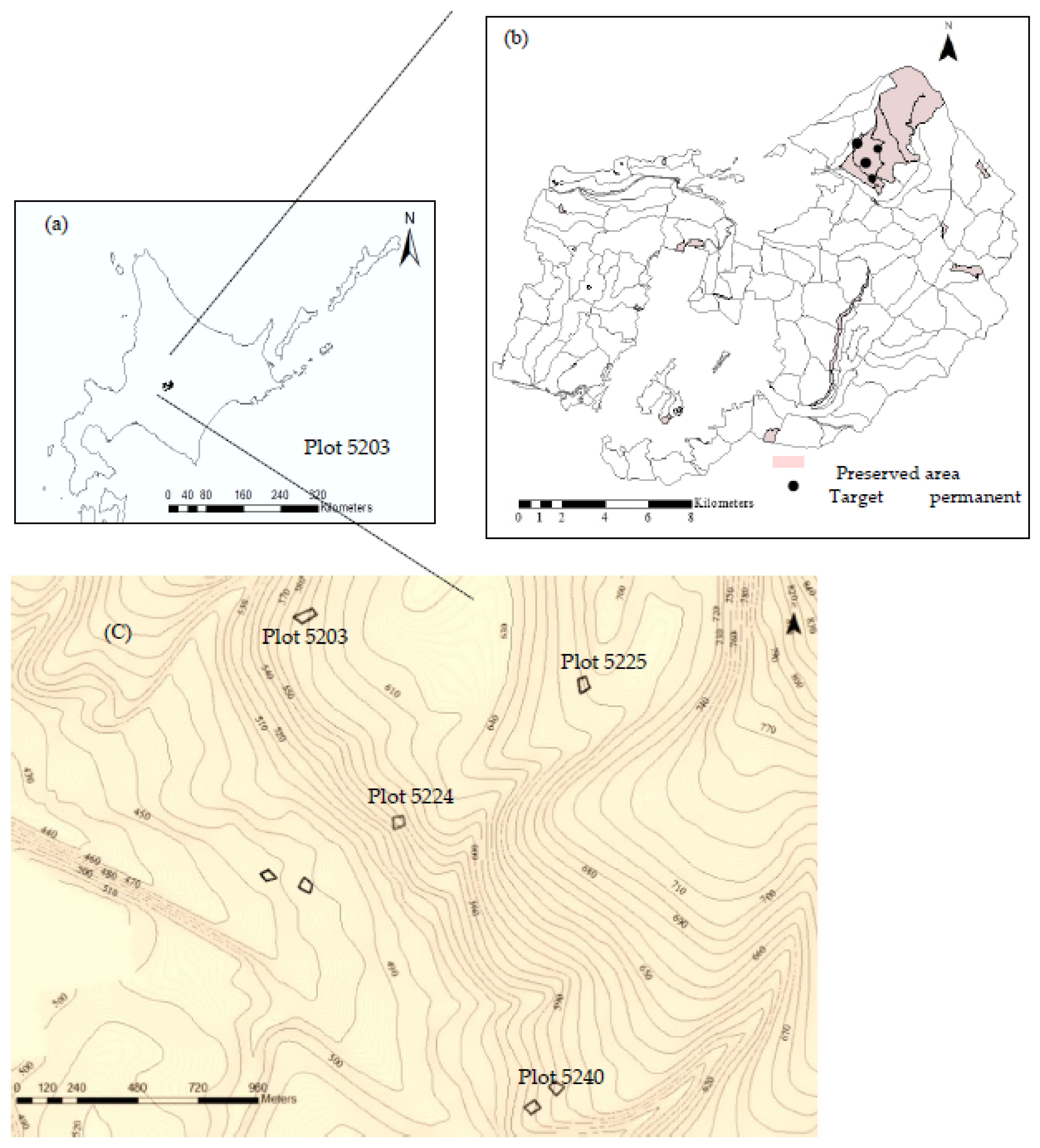
2.1. Study Area

The study area for this research was the UTHF, located at an altitude of 290–1459 m (43°10–20′ N, 142°18–40′ E) in the transition area from deciduous forests in the cool-temperate zone to coniferous forests in the subboreal zone. The total area of the forest was approximately 22,700 ha. The annual rainfall is 1297 mm, and the mean annual temperature is 6.4 °C [16]. The dominant soil types at the study site are Cambisols and Andosols [20]. Through single tree-selection cuttings, diseased, senescent, non-vigorous, unwanted, and deformed trees are removed to control the stand composition toward a desired one. This increases the large-sized trees for periodic harvests and continuously maintains stand volumes at their highest possible level. This system takes advantage of the diversity in the growth, vigor, and longevity of dominant trees from a wide range of tree species found in natural forest ecosystems.

There are ninety-five permanent measurement plots and two long-term ecological research plots in the UTHF. The staff periodically conducts ground forest surveys for spatially explicit stand classification, field measurements of forest inventory plots, and single-tree selection for harvest every year. Stand-scale data of forest resource management are recorded from each investigation. Harvesting and management decisions are based on individual-scale permanent measurement plots. Among these permanent plots, 25 are in the preserved area (size range from 0.04 to 2.25 ha, elevation range 380–1290 m). Diameter at breast height (DBH) measurements of all trees with a DBH ≥ 5 cm are conducted by UTHF staff, and in total, 5-year intervals and census data are available for the last five decades. There has been no human intervention in this preserved area for the last several decades. However, wind, fire, and insect outbreaks are the prevailing natural disturbances in this area.

We selected four plots (#5203, #5224, #5225, and #5240) for our case study, ranging in size from 0.04 to 0.25 ha, located at an elevation range of 570–690 m with similar slope aspects and slope angles (

Table 1. Location and features of the investigated preserved plots of UTHF.

Plot Number	Plot Size (ha)	Elevation (m)	No. of Target Trees in Period 3	Slope Aspect	Mean Slope Angle (°)
5203	0.40	580	327	Southwest	15
5224	0.25	570	150	Southwest	18
5225	0.25	690	237	Southwest	20
5240	0.25	600	214	Southwest	25

; Figure 1). In addition, the stands in the four plots are all classified as the stand type of “coniferous selective cutting with poor regeneration” in the UTHF. This is because selective cuttings of coniferous species have been carried out several times from 1903 to 1957 [21]. The selected plots were in proximity with similar species composition. The characteristic vegetation was coniferous and broad-leaved mixed forests dominated by Abies sachalinensis, Picea jezoensis, Acer spp., and Tilia spp. Among conifer trees, 99% consisted of A. sachalinensis and P. jezoensis. By considering the number of dead trees of each broad-leaved tree species, these were combined for further analysis.

The tree data of the four combined plots, which included 260 A. sachalinensis trees, 139 P. jezoensis trees, and 528 broad-leaved trees, were utilized for prediction model development.

2.2. Collection of Tree Age Data in Observation Periods

Census data for permanent plots in the UTHF are available from 1969 to 2021. We used tree census data (species, DBH, state of being alive or dead, cause of death, etc.) of the four plots measured between 1989 and 2019. In line with the census data, three observation periods were used: 1989–1999 (period 1), 1999–2009 (period 2), and 2009–2019 (period 3). All target trees were alive and had a DBH ≥ 5 cm in 1989, although parts of these trees were already dead by 2019. Based on these census data, the ages of most trees (54%) were identified.

The DBH in centimeters was defined as the in-growth point, and the number of annual rings represented the age after in-growth. By considering the “age after ingrowth”, we can ignore the impact of trees with DBH < 5 cm in later survival analysis [22]. We collected the “tree age after ingrowth” (i.e., the number of annual rings from bark to pith in radius at breast height minus 2.5 cm). A semi-non-destructive device named RESISTOGRAPH (Heidelberg, Germany) was used to detect the annual rings of both living and dead target trees [22]. The measurement data were then extracted using DECOM software (Philadelphia, PA, USA), which can be used to automatically mark tree-ring limits based on the boundaries between early and latewood areas [23]. Wijenayake and Hiroshima [19] developed polynomial equations for the badly rotten, dead trees and living trees of study plots whose ages were unable to be estimated by the RESISTOGRAPH and census data. These equations were used to determine the age after the ingrowth of these trees.

2.3. Survival Analysis

The Kaplan–Meier method computes the likelihood of dying at a certain point in time conditional on survival up to that point [24]. It uses the data of the censored individuals until the object is censored. Thus, it maximizes the utilization of available data at the time to the event of the study sample.

Survival probability functions were developed based on previous studies [22,25,26,27,28,29,30]. Tree mortality is introduced as a stochastic variable (T) that is unique to each target tree. Here, T indicates the age class after ingrowth and is defined as a continuous variable based on the probability density function f(T). One age class represents ten years. If a tree in the t-th age class dies, the conditional probability, called the mortality rate (p_t), can be defined as follows:

$$\mathrm{Pr}(t-1<T\le t|T>t-1)=p_t$$

(1)

If a tree survives in the t-th age class during the observation period, the conditional probability is defined as follows:

$$\mathrm{Pr}(T>t|T>t-1)=1-p_t$$

(2)

By employing the probability density function, the mortality probability (q_t) of new ingrowth trees in the t-th age class is defined as follows:

$$\mathrm{Pr}(t-1<T\le t)={\displaystyle \underset{t-1}{\overset{t}{\int }}f(T)dT=}{q}_t$$

(3)

In addition, the survival probability (r_t) in the t-th age class is defined as follows:

$$\mathrm{Pr}(T>t-1)={\displaystyle \underset{t-1}{\overset{\infty }{\int }}f(T)dT=1-{\displaystyle \underset{1}{\overset{t-1}{\int }}f(T)dT=}}{r}_t$$

(4)

Therefore, based on Equations (1), (3) and (4), the mortality rate $p_t$ can also be

$$p_t=\frac{q_t}{r_t}$$

(5)

By following the methods of Fujikake [31], Hiroshima [32], and Tiryana et al. [33] and considering Equations (1) and (2), we describe the likelihood function (L) of the observation as follows:

$$\begin{gathered} L={\displaystyle \prod _t}\mathrm{Pr}(t-1<T\le t|T>t-1{)}^{d_t} \mathrm{Pr}{(T>t|T>t-1)}^{a_t} \\ ={\displaystyle \prod _t{\left(\frac{{\displaystyle {\int }_{t-1}^{t}f(T)dT}}{{\displaystyle {\int }_{t-1}^{\infty }f(T)dT}}\right)}^{d_t}{\left(\frac{{\displaystyle {\int }_t^{\infty }f(T)dT}}{{\displaystyle {\int }_{t-1}^{\infty }f(T)dT}}\right)}^{a_t}} \end{gathered}$$

(6)

where d_t is the number of dead trees, and a_t is the number of surviving trees in the t-th age class during the observation period.

Thus, Equation (6) can also be expressed as follows:

$$\begin{gathered} L={\displaystyle \prod _t{\left(\frac{{\displaystyle {\int }_{t-1}^{t}f(T)dT}}{{\displaystyle {\int }_{t-1}^{\infty }f(T)dT}}\right)}^{d_t}{\left(\frac{{\displaystyle {\int }_t^{\infty }f(T)dT}}{{\displaystyle {\int }_{t-1}^{\infty }f(T)dT}}\right)}^{a_t}} \\ ={\displaystyle \prod _t}{\left(\frac{q_t}{r_t}\right)}^{d_t}{\left(1-\frac{q_t}{r_t}\right)}^{a_t}={\displaystyle \prod _t}{p}_t{}^{d_t}{(1-p_t)}^{a_t} \end{gathered}$$

(7)

The maximum likelihood estimator of p_t can be calculated by solving the first-order derivation equation in Equation (7) as shown in Equation (8):

$$\stackrel{\wedge }{p_t}=\frac{d_t}{a_t+d_t}$$

(8)

Moreover, considering Equations (4) and (5) leads to

$$r_t-r_{t+1}=q_t$$

(9)

The survival probability can be converted into

$$r_{t+1}=r_t-q_t=r_t\left(1-\frac{q_t}{r_t}\right)=r_t\left(1-p_t\right)$$

(10)

Equation (10) can also be presented as follows:

$$r_t={\displaystyle \prod _{k<t}\left(1-p_k\right)}$$

(11)

This consistent estimator is called the Kaplan–Meier estimate [24], which describes the distribution of survival probabilities.

Based on the results of Wijenayake and Hiroshima [19], stable survival probabilities between periods 2 and 3 for conifer and broad-leaved trees were used for future predictions. Including the age-class distribution of all trees led to a better assessment of the future trends in this forest stand. Furthermore, variations in each age class were reflected by aggregating all trees together. Parametric Weibull distributions were applied to derive the scale parameter, shape parameter, mean, and variance values for the survival data in period 3 separated by three groups of A. sachalinensis, P. jezoensis, broad-leaved trees, and all the trees to smooth the stepwise non-parametric estimates for mean lifetime calculations. For this purpose, we applied the Weibull distribution for f(T) with parameters m and k:

$$f(t;m,k)=\frac{k}{m^k}{t}^{k-1}{e}^{-}{}^{{(\frac{t}{m})}^k}$$

(12)

The mean and variance of the Weibull distribution are $m\Gamma \left(1/k+1\right)$ and $m^2\left\{\Gamma \left(2/k+1\right)-{\Gamma }^2\left(1/k+1\right)\right\}$, respectively; the former represents the mean lifetime. The parameters can also be estimated using the maximum likelihood method with L in Equation (6).

2.4. Future Predictions

Then, the mortality rates were estimated for the tree groups and applied to perform future predictions of living and dead trees for the upcoming 10 periods (100 years) based on Equations (2) and (3):

$$b_t=(a_{t-1}+d_{t-1})(1-p_{t-1}),t\ge 2$$

(13)

$$c_t=(a_{t-1}+d_{t-1})(p_{t-1}),t\ge 2$$

(14)

Here, b_t and c_t represent the number of living and dead trees in the current period by age class t. This is based on the number of living trees a_t, dead trees d_t, and the corresponding tree mortality rate p_t in the previous period. The number of new ingrowth trees was assumed based on the generalized normal forest theory. This theory was developed by Suzuki [34], who described a converged state of the age distribution of a normal forest proportional to the shape of a fixed survival probability curve (the so-called Gentan curve) in the long run. In this theory, he assumed the prediction of new ingrowth trees (he dealt with the reforestation area in the case of forest plantation) as follows:

Total number of dead trees in the previous period = Number of new ingrowth trees in the current period

(15)

Using such scenarios to make decisions about the future is one strategy to understand the identification of harvesting trees, and it stimulates creative thinking on decisions instead of what the future will look like [35]. In the following plantation forests, the concept of Suzuki [34] was applied to predict the new ingrowth of trees in each period. Other than this theoretical scenario (100%), it is essential to attempt various percentages of new ingrowth and dead trees based on existing stable trends; therefore, different scenarios such as 70% and 50% were developed by following sequential calculation methods to predict the future of major conifer trees, broad-leaved trees, and all the trees. Finally, the climax states of major conifers and broad-leaved trees were developed.

3. Results

3.1. Tree Composition and Age-Class Distribution of Major Conifers, Broad-Leaved Trees, and All the Trees

Temporal structural changes were compared and found to be statistically significant over three consecutive periods. The log-rank and Wilcoxon statistical test (

Table 2. Log-rank test and Wilcoxon results of each tree group to compare the three observational periods.

Period	Tree Species
	A. sachalinensis				P. jezoensis				All Broad-Leaved Species
	Log-Rank Test		Wilcoxon Test		Log-rRank Test		Wilcoxon Test		Log-Rank Test		Wilcoxon Test
	p-Value	Chi-Square Value	p-Value	Chi-Square Value	p-Value	Chi-Square Value	p-Value	Chi-Square Value	p-Value	Chi-Square Value	p-Value	Chi-Square Value
Periods 1 and 2	0.9161	0.0111	0.6542	0.2007	0.5023	0.4502	0.3674	0.8124	0.0194 *	5.4637	0.0772	3.1236
Periods 2 and 3	0.1034	2.6524	0.5685	0.3252	0.1538	2.0337	0.2549	1.2961	0.2691	1.2215	0.0610	3.5101

* Indicates a significant difference (p < 0.05).

) results showed that the differences in the mortality of broad-leaved species between periods 1 and 2 were only statistically significant based on the log-rank test (p-value = 0.0194). Furthermore, each comparison had no statistically significant differences among coniferous species. Therefore, period 3 data were applied as the base for future predictions, since there was no significant difference between periods 2 and 1. The numbers of living and dead trees in the major conifers, broad-leaved trees, and all trees in period 3 are presented in

Table 3. Summary of the living and dead trees of major conifer species, broad-leaved trees, and all the trees in period 3.

Tree Category	No. of Trees (%)
	Living Trees	Dead Trees
Conifer
P. jezoensis	117 (12.62)	22 (2.37)
A. sachalinensis	219 (23.62)	41 (4.42)
Broad-leaved	429 (46.28)	99 (10.68)
Total	765 (82.52)	162 (17.48)

. The living and dead tree percentages were 12.62% and 2.37% for P. jezoensis, and those for A. sachalinensis were 23.62% and 4.42%, respectively. Broad-leaved living and dead trees were 46.28% and 10.68%, respectively. Thus, in total, 17.48% of trees were considered dead trees.

The age-class distribution, including dead and living trees of the major conifer and broad-leaved trees in period 3, is presented in Figure 2. The first age class represents the new ingrowth trees of each species category; most of them are broad-leaved trees.

P. jezoensis represents a multimodal age-class distribution throughout all age classes. The age distribution of A. sachalinensis formed an exponential shape, with a few exceptions in the fourth and fifth age classes. Broad-leaved trees showed a similar exponential shape over age classes, except for the first age class. All trees in the sampled plots represented an exponential shape, with a few exceptions in age classes 1, 4, and 8.

3.2. Survival Analyses

The estimated Weibull parameters of m and k and the mean and standard deviation are listed in

Table 4. Age-class probability Weibull distributions for major conifer species and broad-leaved trees.

Weibull Parameter	P. jezoensis	A. sachalinensis	Broad-Leaved	All Trees
m	6.7133	7.3496	6.0360	6.8872
k	1.1600	1.3525	0.7279	0.9144
Mean	6.3732	6.7374	7.3722	7.1851
Standard Deviation	5.5101	5.0359	10.3135	7.5409

. The mortality probability, mortality rate, and survival probabilities were calculated for each group using the respective Weibull parameters, and the results are shown in Figure 3. The shape parameters differed in the range of k < 1 for broad-leaved trees and k > 1 for P. jezoensis and A. sachalinensis, leading to differences in the shape of the curves. These differences in shape resulted in a difference in the mean lifetime of 64 years in P. jezoensis, 67 in A. sachalinensis, and 74 years in broad-leaved trees due to different mortality rates between conifer and broad-leaved trees. Interestingly, both P. jezoensis and A. sachalinensis showed different patterns for the mortality rate, which led to an increasing trend along with the age class, which came from the different range of shape parameters k > 1 for period 3. In period 3, broad-leaved trees (Figure 3c) showed decreasing trends in mortality and survival probabilities along with age classes. Broad-leaved species represented the highest mortality probability and mortality rate values in the first age class, fell mainly in the second age class, and then decreased steadily with an increase in age. Figure 3d depicts the rates of mortality, survival, and mortality probability at each age class by considering the three groups together. Based on the survival probability values of P. jezoensis, A. sachalinensis, broad-leaved trees, and all trees, the probability of a tree to survive until age 40 was, for instance, 68%, 74%, 55%, and 63%, respectively. However, when considering a survival time of 180 years, survival probabilities were 5%, 4%, 12%, and 10%, respectively.

The living-tree distributions of each category of the previous period were calculated based on the Weibull models of period 3 (

Table 5. Root mean square and root mean square percentage values of each category based on prediction of living trees of period 2 of all sampled plots.

Tree Category	Period 2
	RMSE Living Trees	RMSPE (%) Living Trees
P. jezoensis	1.20	23.31
A. sachalinensis	1.30	8.96
Broad-leaved	4.91	36.67
All trees	6.28	17.08

, Figure 4) for validation. Predictions of dead trees are basically underestimated for younger and older age classes and slightly overestimated for the middle class. The resulting living trees and actual tree numbers of each age class were compared in terms of the root mean square error (RMSE) and root mean square percentage error (RMSPE) to determine the validity of the predictions. This exhibited a better prediction power for each category as follows: A. sachalinensis had the lowest RMSE (1.20 living trees) value, whereas all the trees (6.28 living trees) had the highest value. The RMSE results correctly represented the characteristics of age distributions, which showed that the validation results were sufficiently precise.

Figure 5 represents the future age distribution of each major conifer, broad-leaved trees, and all tree species for the upcoming 10 periods (periods 4 to 13) by considering the theory of Suzuki [34]. Sequentially, a higher number of tree mortalities occurred in younger age classes than that for older age classes in conifer and broad-leaved trees during the study period. When considering time-series changes in age distributions from periods 4 to 13, the theoretical exponential shapes, which were proportional to the survival probabilities in Figure 3, were gradually revealed in younger age classes, and finally, the theoretical shapes were achieved by the 10th age class of major conifer, broad-leaved trees, and all trees in period 13. In addition, as time passed, the number of living conifer and broad-leaved trees gradually increased from period to period.

Figure 6 shows the climax state of conifer and broad-leaved trees based on the generalized normal forest theory. The upper limit of age classes was determined based on the mean biological age [36] of the stand. The tree composition of conifer and broad-leaved trees was in a stable state with an exponential shape of the climax state of the stand. The tree species composition along the age classes became closer and reached a mature state.

By assuming only 70% of dead trees in the previous period to be equivalent to the number of new ingrowth trees in the next period, future predictions were carried out for the next 100 years (Figure 7). For example, in this scenario, three A. sachalinensis trees that belong to the third age class will die in the period 2019–2029 (period 4 of Figure 7). By period 13, all distributions of tree categories reached exploitational and multi-modal shapes.

Moreover, by assuming that only 50% of dead trees of the previous period were equivalent to new ingrowths of the next period, future predictions were carried out for the next 100 years (Figure 8). By period 13 of the 50% scenario, all tree categories represent the multi-modal shape of the age-class distribution.

4. Discussion

The prediction and modeling of natural forests help determine the possibility of optimal forest management to achieve a desirable structure and sustainability of forests [37]. The single-tree cutting system that the UTHF follows is based on the strategy of early identification of likely dead trees. However, a lack of suitable decision-support tools can delay the proper implementation of uneven management in mixed broad-leaved forests [38].

To achieve more accurate lifetime estimations, it is crucial to analyze the age at the time of death [39]. Prerequisite conditions, such as the stability of survival probability over time, can lead to a proper prediction of living and dead trees in the future. In this study, the predictions of living and dead trees were validated based on the 1999–2009 period. Subsequently, predictions were made for the upcoming ten periods under various scenarios other than Suzuki’s [34] theory. Predicting future forest dynamics on a stand-scale is vital for sustainable forest management [40]. This study predicted the future age distribution for a 100-year period based on the current period of three situations for each tree category. Parametric survival characteristics of period 3 for P. jezoensis, A. sachalinensis, and broad-leaved trees were the basis for the predictions. All tree predictions can be used as representative pictures of the whole stand.

4.1. Stand Dynamics

In this study (Figure 5), a higher number of tree mortalities occurred in the younger age classes than in the older age classes over time. The predicted age distributions nearly converged (up to the 10th age class) to a theoretical shape proportional to the survival probability curve in this 100% scenario. The period in which the shape of the age distribution converges to the theoretical shape of the survival probability curve can be considered as the reaching point of the climax state of the forest stand, because the composition of the tree species and the age distribution become completely stable over time.

The multi-modal age class distribution of P. jezoensis was predominant among all the prediction scenarios, whereas the exponential shape of A. sachalinensis age distribution in the 100% scenario gradually shifted to a multimodal shape in the 50% scenario prediction. In addition, the exponential shape of all the trees in the 100% scenario gradually changed to multi-modal by achieving nearly actual perspectives. P. jezoensis exclusively regenerates on substrates such as fallen logs; thus, it can be a critical factor for determining natural regeneration [41]. Kubota et al. [42] reported that A. sachalinensis can grow taller than P. jezoensis under suppressed conditions, whereas P. jezoensis requires canopy gaps for steady height growth. Whitmore [43] suggested that the genus Abies tolerates shade, is of late succession, and finally, forms climax communities. Moreover, Kubota and Hara [42] suggested that the regeneration pattern related to light environments differs between the two species with distinct crown shapes. Therefore, habitat segregation, substrate abundance, and the number of new ingrowths of major conifer species were determined during the early stages of life history. Fewer P. jezoensis were observed throughout all periods when compared to A. sachalinensis. Takahashi et al. [44] found that A. sachalinensis was predominant in areas below 700 m, whereas P. jezoensis was dominant in comparatively higher areas and cooler locations. Therefore, the coexistence of major conifer species affected the age-class distribution pattern of this study area.

Harvesting behavior can be determined based on the number of new ingrowths and dead trees in each period. Suzuki’s generalized normal forest theory for plantation forests [34] was used to determine the future of natural forests. Although the number of new ingrowths and dead trees can differ in each period depending on various factors, such as typhoons, diseases, and natural mortalities, it is essential to incorporate these factors as well. When we predict the future, the exact number of new ingrowth trees of each age class cannot be revealed following this Suzuki theory. In that sense, it is worth having several scenarios to understand the future of the natural forest, and it would be a conceivable approach for predicting future age distribution. Therefore, we included not only the 100% scenario, but also the 70% and 50% scenarios. Both the 70% and 50% scenarios attempted to reach a realistic approach; however, the 70% scenario remained theoretical to some extent, and an exponential shape of age distribution was observed, whereas the 50% scenario showed a multimodal shape of age distribution throughout the predictions. Lähde et al. [45], Hörnberg [46], and Zackrisson et al. [47] indicated that old-growth forests have a multimodal tree-age distribution, which is a critical feature of old-growth forests. In terms of this perspective, the 50% scenario can be considered the old-growth forest approach. During each period, both conifer species and broad-leaved trees had various proportions of living and dead trees. In the meantime, this is getting closer to the old-growth approach, especially in the latter periods of 50% scenario. In this sense, resultant predictions of a 50% scenario can be a more robust and realistic approach for determining the harvesting behavior of undesired trees to maintain the SSMS of UTHF.

4.2. Management Implications for SSMS

The natural mortality of trees is minimized following the SSMS by preferentially harvesting trees that would otherwise die [48]. The SSMS helps sustain tree health and productivity and controls the stand composition. The existing literature on UTHF did not suggest stand-age distribution in natural forest stands; therefore, it is meaningful to fill this gap by incorporating survival probability techniques in natural forest stands to predict living and dead trees based on age classes for the upcoming years.

This study investigated future predictions based on stable survival probabilities in period 3 of each major tree category of the UTHF. Forest managers can rely on these predicted age-class distributions for decision making, such as harvesting tree selection based on the SSMS. The resulting prediction of dead trees based on age classes will serve as a harvesting indicator before tree death. For instance, seven A. sachalinensis trees belonging to the seventh age class could possibly die in the period 2059–2069 (period 8 of Figure 5). Thus, we can perform close supervision of the growth and external behavior when the trees reach that age class (after age information is converted into DBH information using the equations developed by Wijenayake and Hiroshima [19]), because they are likely to die in the near future. The early identification of likely-to-die trees may lead to a better understanding of the future of the forest, thereby facilitating inventory preparation as well.

The SSMS keeps stands in the state of the pre-climax stage to improve the vigor of upper-story trees, which allows a high growth rate at the stand level

Age-class distribution of the climax state in the 100% scenario could be described as the most significant stable state of this forest stand type. To date, it is theoretically possible to maintain stands under the pre-climax stage by allowing enough new ingrowth at the stand level. In the long run, the converged state of the age distribution of a generalized normal forest is theoretically proportional to the shape of the stable survival probability curve [34] (Suzuki, 1984).

Thus, predictions of the age-class distribution of each plot in this study can be used as site-specific management plans to identify living and dead trees of each age class in the future. Furthermore, these predictions can be utilized as a support tool for modeling silvicultural management scenarios to produce management plans that can be applied as a promising means for sustainable forest management. Finally, the findings of this study contribute valuable information to assist in forest planning with robust and comprehensive results.

However, there are limitations to the practical application of these scenarios. Under actual conditions, the dead tree predictions of each age class can vary owing to external disturbances such as typhoons, diseases, and other related factors. To minimize such errors, it is essential to incorporate these factors through modeling. Another alternative is to carry out back-casting based on developed mortality rates. The model results and actual results can then be compared prior to use, and this may lead to a better understanding of the accuracy of future projections. The future predictions of living and dead trees were derived using generalized normal forest theory [34]. However, this theoretical assumption is rare in the field. Therefore, other ingrowth assumptions are required based on the census data of long-term permanent plots. In addition, it is necessary to apply this theory to different stand types in the SSMS. This may enhance the validity of the predicted age-class distributions of the upcoming periods. As this study showed the applicability of the survival analysis methodology on future predictions of natural forests, it would be better to examine it further by considering factors such as species, cause of death, and effect of climate changes in different natural forest stands. Advantageously, the predicted age-class distributions represent the stand degradation of the major tree species.

5. Conclusions

This study applied age-based survival analyses to natural forest stands to predict future age distribution by following parametric analysis with several scenarios for major conifer species and broad-leaved trees of preserved forests in northern Hokkaido. Stable survival probabilities between periods 2 and 3 for each conifer and broad-leaved category led to further analysis of future age predictions of the stands. We also estimated the age distribution of the climax states of the major tree species.

The exponential shape of age-class distribution shifted to the multi-modal distribution of A. sachalinensis and broad-leaved trees in the 50% scenario, whereas P. jezoensis had the same multi-modal distribution patterns throughout the scenarios. Furthermore, the two dominant conifer species showed different age-class distribution trends, especially in early life. The predicted age distributions nearly converged to the shape of the survival probability curve. In the long run, the species composition of conifer and broad-leaved trees and their age distribution would reach stable states, assuming the generalized normal forest theory. The species composition of conifer and broad-leaved trees and their age distribution would be stable in the long term by reaching a climax state. To date, it is theoretically possible to maintain stands under the pre-climax stage by allowing enough new ingrowth at the stand level. The developed model can be used as a support tool for modeling silvicultural management scenarios to produce management plans that can be applied as suitable standards for sustainable forest management in the UTHF. Therefore, the suggested age-class prediction of living and dead trees has the potential to improve the natural forest management of the UTHF. However, low model precision of most tree groups may result in the recommendation of cutting large trees, especially, which can be an overestimation.

References

1. Angelstam, P.K. Maintaining and Restoring Biodiversity in European Boreal Forests by Developing Natural Disturbance Regimes. J. Veg. Sci. 1998, 9, 593–602. [Google Scholar] [CrossRef]
2. Kuuluvainen, T.; Penttinen, A.; Leinonen, K.; Nygren, M. Statistical Opportunities for Comparing Stand Structural Heterogeneity in Managed and Primeval Forests: An Example from Boreal Spruce Forest in Southern Finland. Silva Fenn. 1996, 30, 315–328. [Google Scholar] [CrossRef] [Green Version]
3. Zenner, E.K.; Hibbs, D.E. A New Method for Modeling the Heterogeneity of Forest Structure. For. Ecol. Manag. 2000, 129, 75–87. [Google Scholar] [CrossRef]
4. Agren, J.; Zackrisson, O. Age and Size Structure of Pinus Sylvestris Populations on Mires in Central and Northern Sweden. J. Ecol. 1990, 78, 1049. [Google Scholar] [CrossRef]
5. Limaei, S.M.; Lohmander, P.; Olsson, L. Dynamic Growth Models for Continuous Cover Multi-Species Forestry in Iranian Caspian Forests. J. For. Sci. 2017, 63, 519–529. [Google Scholar] [CrossRef] [Green Version]
6. Wallenius, T.; Kuuluvainen, T.; Heikkilä, R.; Lindholm, T. Spatial Tree Age Structure and Fire History in Two Old-Growth Forests in Eastern Fennoscandia. Silva Fenn. 2002, 36, 185–199. [Google Scholar] [CrossRef] [Green Version]
7. Paul, C.; Brandl, S.; Friedrich, S.; Falk, W.; Härtl, F.; Knoke, T. Climate Change and Mixed Forests: How Do Altered Survival Probabilities Impact Economically Desirable Species Proportions of Norway Spruce and European Beech? Ann. For. Sci. 2019, 76, 14. [Google Scholar] [CrossRef] [Green Version]
8. Moe, K.T.; Owari, T. Sustainability of High-Value Timber Species in Mixed Conifer-Broadleaf Forest Managed under Selection System in Northern Japan. Forests 2020, 11, 484. [Google Scholar] [CrossRef]
9. Watt, A.S. Pattern and Process in the Plant Community. J. Ecol. 1947, 35, 1–22. [Google Scholar] [CrossRef] [Green Version]
10. Villalba, R.; Veblen, T.T. Regional Patterns of Tree Population Age Structures in Northern Patagonia: Climatic and Disturbance Influences. J. Ecol. 1997, 85, 113–124. [Google Scholar] [CrossRef]
11. Antos, J.A.; Parish, R.; Conley, K. Age Structure and Growth of the Tree-Seedling Bank in Subalpine Spruce-Fir Forests of South-Central British Columbia. Am. Midl. Nat. 2000, 143, 342–354. [Google Scholar] [CrossRef]
12. Worbes, M.; Staschel, R.; Roloff, A.; Junk, W.J. Tree Ring Analysis Reveals Age Structure, Dynamics and Wood Production of a Natural Forest Stand in Cameroon. For. Ecol. Manag. 2003, 173, 105–123. [Google Scholar] [CrossRef]
13. Loewenstein, E.F.; Johnson, P.S.; Garrett, H.E. Age and Diameter Structure of a Managed Uneven-Aged Oak Forest. Can. J. For. Res. 2000, 30, 1060–1070. [Google Scholar] [CrossRef]
14. Yue, Q.; Hao, M.; Li, X.; Zhang, C.; von Gadow, K.; Zhao, X. Assessing Biotic and Abiotic Effects on Forest Productivity in Three Temperate Forests. Ecol. Evol. 2020, 10, 7887–7900. [Google Scholar] [CrossRef] [PubMed]
15. Takahashi, N. The Stand-Based Silvicultural Management System: Its Theory and Practices, 1st ed.; Log Bee: Sapporo, Japan, 2001. [Google Scholar]
16. The University of Tokyo Hokkaido Forest. 2021. Available online: http://www.uf.a.u-tokyo.ac.jp/files/gaiyo_hokkaido.pdf. (accessed on 26 July 2020).
17. Owari, T.; Yasumura, N.; Ishibashi, S.; Kamoda, S.; Saito, H. The University of Tokyo Forests and Forest Science Education in Japan; SILVA Network Conference. Faculty of Forestry and Wood Sciences; Czech University of Life Sciences: Prague, Czech, 2019; pp. 38–50. [Google Scholar]
18. Wijenayake, P.R.; Hiroshima, T. Survival Analyses of Individual Tree Populations in Natural Forest Stands to Evaluate the Maturity of Forest Stands: A Case Study of Preserved Forests in Northern Japan. J. For. Plan. 2022, 28, 1–13. [Google Scholar] [CrossRef]
19. Wijenayake, P.R.; Hiroshima, T. Age-based Survival Analysis of Coniferous and Broad-leaved Trees: A Case Study of Preserved Forests in Northern Japan. Forests 2021, 12, 1014. [Google Scholar] [CrossRef]
20. IUSS Working Group WRB-FAO. World Reference Base for Soil Resources 2014, Update 2015. International Soil Classification System for Naming Soils and Creating Legends for Soil Maps; IUSS Working Group WRB-FAO: Rome, Italy, 2015. [Google Scholar]
21. Nakagawa, M.; Kurahashi, A.; Kaji, M.; Hogetsu, T. The Effects of Selection Cutting on Regeneration of Picea Jezoensis and Abies Sachalinensis in the Sub-Boreal Forests of Hokkaido, Northern Japan. For. Ecol. Manag. 2001, 146, 15–23. [Google Scholar] [CrossRef]
22. Hiroshima, T. Applying Age-Based Mortality Analysis to a Natural Forest Stand in Japan. J. For. Res. 2014, 19, 379–387. [Google Scholar] [CrossRef]
23. Rinn, F. Eine Neue Bohrmethode Zur Holzuntersuchung. Holz-Zent. 1989, 34, 529–530. [Google Scholar]
24. Kaplan, E.L.; Meier, P. Nonparametric Estimation from Incomplete Observations. J. Am. Stat. Assoc. 1958, 53, 457–481. [Google Scholar] [CrossRef]
25. Kalbfleisch, J.D.; Prentice, R.L. The Statistical Analysis of Failure Time Data; John Wiley and Sons: New York, NY, USA, 1980. [Google Scholar]
26. Cox, D.R.; Oakes, D. Analysis of Survival Data; Chapman and Hall: London, UK, 1984. [Google Scholar]
27. Crowder, M.J.; Kimber, A.C.; Smith, R.L. Statistical Analysis of Reliability Data; Chapman and Hall: London, UK, 1994; Volume 27. [Google Scholar]
28. Klein, J.P.; Moeschberger, M.L. Survival Analysis: Techniques for Censored and Truncated Data; Springer: New York, NY, USA, 1997. [Google Scholar]
29. Kleinbaum, D.G.D.; Klein, M. Statistics for Biology and Health. In Survival Analysis: A Self-Learning Text, 3rd ed.; 2011; ISBN 1441966455. [Google Scholar]
30. Fujikake, I. An Analyses of Harvesting Activities in a Forest Management Entity Using Harvesting Age Distribution (Tentative Translation by Author). Ph.D. Thesis, Kyoto University, Kyoto, Japan, 2000. [Google Scholar]
31. Fujikake, I. Estimation of Gentan Probability Based on the Forest Resource Table. Proc. Inst. J. Stat. Math. 2003, 51, 95–109. [Google Scholar] [CrossRef]
32. Hiroshima, T. Study on the Methodology of Calculating Mean and Variance of Felling Age in Forest Planning. Jpn. J. For. Plan. 2006, 40, 139–149. [Google Scholar] [CrossRef]
33. Tiryana, T.; Tatsuhara, S.; Shiraishi, N. Empirical Models for Estimating the Stand Biomass of Teak Plantations in Java, Indonesia(Multipurpose Forest Management). J. For. Plan. 2011, 16, 35–44. [Google Scholar] [CrossRef]
34. Suzuki, T. The Gentan Probability, a Model for the Improvement of the Normal Forest Concept and Forest Planning. In Proceedings of the IUFRO Symposium on Forest Management Planning and Managerial Economics, Tokyo, Japan, 15–19 October 1984; pp. 12–24. [Google Scholar]
35. Wollenberg, E.; Edmunds, D.; Buck, L. Using Scenarios to Make Decisions about the Future: Anticipatory Learning for the Adaptive Co-Management of Community Forests. Landsc. Urban Plan. 2000, 47, 65–77. [Google Scholar] [CrossRef]
36. Sadamoto, W. Hokkaido Natural Forest Sucession Pattern 1. Hokkaido For. 1970, 261, 349–356. [Google Scholar]
37. Zhao, J.; He, C.; Qi, C.; Wang, X.; Deng, H.; Wang, C.; Liu, H.; Yang, L.; Tan, Z. Biomass Increment and Mortality Losses in Tropical Secondary Forests of Hainan, China. J. For. Res. 2019, 30, 647–655. [Google Scholar] [CrossRef]
38. Bourque, C.P.A.; Bayat, M.; Zhang, C. An Assessment of Height–Diameter Growth Variation in an Unmanaged Fagus Orientalis-Dominated Forest. Eur. J. For. Res. 2019, 138, 607–621. [Google Scholar] [CrossRef]
39. Selvin, S. Statistical Analysis of Epidemiologic Data; Oxford University Press: Oxford, UK, 2004; ISBN 9780199865697. [Google Scholar]
40. Thurnher, C.; Klopf, M.; Hasenauer, H. MOSES—A Tree Growth Simulator for Modelling Stand Response in Central Europe. Ecol. Modell. 2017, 352, 58–76. [Google Scholar] [CrossRef]
41. Narukawa, Y.; Iida, S.; Tanouchi, H.; Abe, S.; Yamamoto, S.I. State of Fallen Logs and the Occurrence of Conifer Seedlings and Saplings in Boreal and Subalpine Old-Growth Forests in Japan. Ecol. Res. 2003, 18, 267–277. [Google Scholar] [CrossRef]
42. Kubota, Y.; Hara, T. Allometry and Competition between Saplings of Picea Jezoensis and Abies Sachalinensis in a Sub-Boreal Coniferous Forest, Northern Japan. Ann. Bot. 1996, 77, 529–538. [Google Scholar] [CrossRef] [Green Version]
43. Whitmore, T.C. Canopy Gaps and the Two Major Groups of Forest Trees. Ecol. Soc. Am. 2009, 70, 536–538. [Google Scholar] [CrossRef]
44. Takahashi, M.; Takao, G.; Ishibashi, S.; Kawahara, T. Evaluation of Landscape-Level Genetic Diversity in Mixed Managed Forest in Hokkaido, Japan. J. For. Plan. 2011, 16, 215–221. [Google Scholar]
45. Lähde, E.; Laiho, O.; Norokorpi, Y.; Saksa, T. The Structure of Advanced Virgin Forests in Finland. Scand. J. For. Res. 1990, 6, 527–537. [Google Scholar] [CrossRef]
46. Hoernberg, G. Boreal Old-Growth Picea Abies Swamp-Forests in Sweden—Disturbance History, Structure and Regeneration Patterns-Thesis; Sveriges Lantbruksuniversitet: Uppsala, Sweden, 1996. [Google Scholar]
47. Zackrisson, O. Influence of Forest Fires on the North Swedish Boreal Forest. Oikos 1977, 29, 22–32. [Google Scholar] [CrossRef]
48. Yamamoto, H. Natural Forest Management Based on Selection Cutting and Natural Regeneration. In Proceedings of the IUFRO International Workshop on Sustainable Forest Managements, Furano, Japan, 17–21 October 1994; pp. 10–22. [Google Scholar]
Figure 1. Study area and selected plots. (a) University of Tokyo Hokkaido Forest (UTHF); (b) targeted permanent plots of the persevered area; (c) contour map of surrounding of the selected plots.
Forests 13 01912 g001
Figure 2. Age-class distributions of living and dead trees of major conifer species, broad-leaved trees, and all the trees of 4 study plots in period 3.
Forests 13 01912 g002
Figure 3. Distribution of tree mortality probability, mortality rate, and survival probability based on Weibull distributions: (a) A. sachalinensis, (b) P. jezoensis, (c) broad-leaved trees, and (d) all trees.
Forests 13 01912 g003
Figure 4. Observed and predicted age class distribution (a) P. jezoensis, (b) A. sachalinensis, and (c) broad-leaved trees.
Forests 13 01912 g004aForests 13 01912 g004b
Figure 5. Future prediction results (100% scenario) of upcoming 100 years of conifer and broad-leaved trees; the rest of the periods are attached to the Supplementary Materials.
Forests 13 01912 g005
Figure 6. Climax state of major conifer species, broad-leaved trees, and all the trees.
Forests 13 01912 g006
Figure 7. Future prediction results (70% scenario) of upcoming 100 years of conifer and broad-leaved trees; the rest of the periods are attached to the Supplementary Materials.
Forests 13 01912 g007
Figure 8. Future prediction results (50% scenario) of upcoming 100 years of conifer and broad-leaved trees; the rest of the periods are attached to the Supplementary Materials.
Forests 13 01912 g008