Article

Effects of Edaphic Factors at Different Depths on β-Diversity Patterns for Subtropical Plant Communities Based on MS-GDM in Southern China

Guangzhou Institute of Geography, Guangdong Academy of Sciences, Guangzhou 510070, China
*
Author to whom correspondence should be addressed.
Forests 2022, 13(12), 2184; https://doi.org/10.3390/f13122184
Submission received: 26 October 2022 / Revised: 10 December 2022 / Accepted: 12 December 2022 / Published: 19 December 2022
(This article belongs to the Special Issue Maintenance of Forest Biodiversity)

Abstract

:
Previous research on the relationship between edaphic factors and species diversity patterns has mostly focused on topsoil between 0 and 30 cm, with less attention paid to deeper layers where many plant root systems are concentrated. Since considering deeper edaphic layers might help to unravel the maintenance mechanisms of plant diversity, in the present study we explored the relationship between vegetation β-diversity and a comprehensive set of soil chemical attributes at different depths. Based on vegetation and soil data from subtropical broad-leaved forest plots in the Nanling Mountains, China, we analyzed the driving factors of β-diversity patterns of trees, shrubs, and herbs using multi-site generalized dissimilarity modeling (MS-GDM). We found that the species composition dissimilarity of trees, shrubs, and herbs layers in the study area was highly diversified and dominated by species turnover components. Topsoil chemical properties were the best explainers for the β-diversity of trees (52.5%), followed by herbs (40.3%) and shrubs (21.8%). With the increase of soil depth, especially for depth >60 cm, soil chemical elements gradually lost explanatory power. Regarding the β-diversity of trees, it was mainly affected by altitude and available nitrogen (AN), total iron (Fe), and nickel (Ni) content in the soil of 0–60 cm depth. Concerning shrubs, the best β-diversity explainers were altitude, geographical distance, and nutrient elements of the soil above 40 cm. The main factors driving the β-diversity of herbs were altitude, total boron (B), total cadmium (Cd), and total nickel (Ni) of 0–40 cm soil. Overall, our results suggest that the environmental filtration process driven by altitude and soil factors, and dispersal limitations represented by geographical distance, affected the β-diversity patterns of Nanling forest communities.

1. Introduction

Biodiversity patterns and changes driven by influencing factors are the core contents of biodiversity research, and studies about biodiversity patterns and mechanisms are conducive to the conservation and sustainable use of biodiversity [1,2]. As a link between local biodiversity (α-diversity) and regional biodiversity (γ-diversity), β-diversity quantifies the changes in species composition and diversity along time or space, which has been widely used in the study of biodiversity in terrestrial and aquatic ecosystems [3,4,5]. Admittedly, the spatial patterns of β-diversity are mainly affected by geographic distance and environmental heterogeneity between sites, reflecting the underlying processes of dispersal limitation and environmental filtering, respectively [6,7,8]. Since β-diversity is key to analyzing species-environment relationships, understanding the geographic patterns of β-diversity and their driving factors is essential to unravelling the mechanisms of species diversity change [9].
β-diversity is generally measured with indices representing pairwise dissimilarity, such as the Jaccard and Sørensen dissimilarity indices, which are divided into two components: species turnover and nestedness [10]. Species turnover describes the degree of species replacement between communities, while nestedness indicates that communities with low richness result from species loss in communities with high richness. Measuring the rate of change in species composition is a common method for testing species turnover. In general, as the spatial distance increases, the similarity of species composition between plots decreases (or the difference increases) [11]. Explanations for this distance-decay relationship include deterministic responses of species to biotic and abiotic conditions (e.g., niche differentiation and competitive asymmetry), as well as spatial processes by which species find suitable environments (e.g., dispersal capability) [5,7,12]. For example, Zhang et al. [13] found that environmental heterogeneity mainly affected the species richness of the Gutianshan forest plot, while spatial processes dominated the species diversity in the Barro Colorado Island forest plot. Environmental differences between communities cause species to exhibit complementary effects on resource use, occupy additional niche space at different locations, and affect β-diversity [5].
Environmental factors such as soil and physiography usually dominate species distribution patterns at regional scales [14,15,16]. Among them, the soil, which contains the nutrient elements required for plant growth and often exhibits strong spatial heterogeneity, is widely believed to promote species coexistence and diversity patterns by increasing niche availability and providing shelters and refuges [17,18]. Early studies provided evidence for edaphic heterogeneity accounting for most of the variation in species richness and species distributions of plant communities [19,20,21]. Zhang et al. [22] found that soil heterogeneity could explain 88.2% of the tree species distribution in the Gutianshan subtropical forest. Hall et al. [23] found that the distribution patterns of four species of Entandrophragma Genus were closely related to soil nutrients (Ca, Mg, and P) in a 100-ha forest plot in Africa. In addition, the diversity in the vertical distribution of plant roots corresponds to different plant strategies for soil resource absorption, which is tightly related to species composition [24,25,26]. Previous studies on the relationship between species diversity patterns and environmental factors mainly focus on 0–10 cm topsoil or 0–30 cm soil layers and pay less attention to the middle and deeper layers where 50% of tree roots are distributed [27]. Therefore, analyzing the effects of soil physicochemical properties on species diversity patterns at different depths will help to better understand the driving mechanisms of biodiversity [13].
In the present study, we simultaneously investigated (i) the relationship between turnover and nestedness components of β-diversity and their environmental correlates of different plant forms (trees, shrubs and herbs) and (ii) the effects of soil physicochemical properties at different depths on β-diversity patterns. Additionally, the ‘dispersal limitation’ and ‘environmental filtering’ hypotheses were examined to explain the influencing mechanism of β-diversity in the well-preserved natural subtropical broadleaved forests of the Nanling Mountains, in the south of China, We used multi-site generalized dissimilarity modeling to analyze the effects of geographic distances, altitude and soil chemical properties of four depth layers on β-diversity patterns of different plant forms, and quantified the effects of environmental factors on β-diversity components (turnover and nestedness). Research results could provide scientific basis for the conservation of biodiversity and forest ecosystems in the Nanling Mountains.

2. Material and Methods
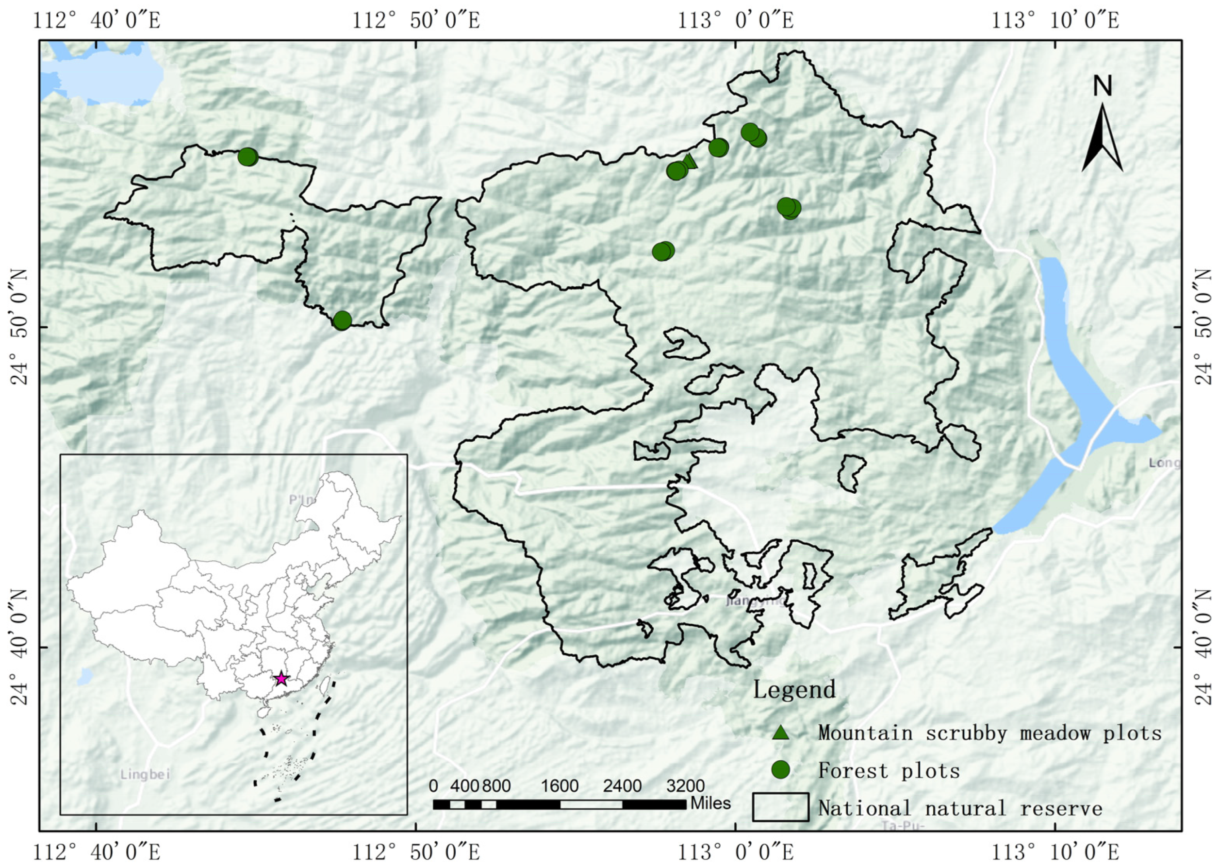
2.1. Study Area

The study area is located in the Nanling National Nature Reserve in the north of Guangdong Province, China, in the middle of the Nanling Mountains. The area spans three counties (cities) of Shaoguan and Qingyuan city, namely Ruyuan, Yangshan and Lianzhou, with 24°37’ N–24°57’ N, 112°30’ E–113°04’ E, and covers an area of 58,400 ha. The highest peak in the area is Shikeng Kong, which is 1902 m above sea level and has a relative elevation difference of 1489 m. The vegetation types of the Nanling Mountains range from subtropical broad-leaved forest, mixed coniferous and broad-leaved forest, and mountain broad-leaved brushwood. The study area shows transitional monsoon climate between Central Asia and South Asia. The annual average temperature is 17.7 °C, with an extreme minimum temperature of −4.2 °C and the extreme maximum temperature of 34.4 °C, with the annual average frost-free period 276 days. The annual average precipitation is 1705 mm, with the annual average relative humidity 84%. Additionally, the precipitation is mostly concentrated from March to October, accounting for about 82% of the annual rainfall. The soils of reserve are mainly red soil, yellow soil and mountain scrubby-meadow soil.
In 2017, 21 forest dynamic plots (40 m × 40 m) and three mountain scrubby-meadow dynamic plots (20 m × 20 m) following the Center for Tropical Forest Science of China (CTFS) standard census protocols were established in Nanling National Nature Reserve (Figure 1). The vegetation types of the plots included evergreen broad-leaved forest, evergreen coniferous broad-leaved mixed forest, mountain evergreen broad-leaved dwarf forest and mountain scrubby meadow (see Table S1 for details on the specific composition of these communities). Each plot was divided into four quadrats as vegetation survey units (20 × 20 m quadrats for forest plots and 10 × 10 cm for the mountain scrubby-meadow plots). Each forest plot included three 2 m × 2 m shrub plots and three 1 m × 1 m herb plots. All the woody stems with ≥1 cm diameter at breast height 1.3 m (DBH) in the plot were mapped, identified and their DBH, total height and crown width measured. The shrub species and saplings with DBH < 1 cm and height > 50 cm in the shrub plots were considered as shrub layer, and their species name, basal diameter and plant height were recorded. Regarding the herb plots, all the herbaceous plants, lianas, and seedlings of trees and shrubs with height < 50 cm were considered as herb layers, and their species name, plant number and height were also recorded.

2.2. Soil Sampling and Analysis

In 2017, a 12 m × 15 m soil fixed observation plot was set near each fixed forest plot, which was divided into six 5 × 6 m subplots for stratification (0–20, 20–40, 40–60, 60–100 cm) sampling using soil drill. Each soil sample is a mixed sample composed of eight-ten samples from the six subplots according to the depth of the same depth layer. Consequently, every soil sample of a specific depth layer has six measurement repetitions. From each sample, 22 chemical soil properties were measured. The results included Total Nitrogen (TN), Total Phosphorus (TP), Total Potassium (TK) and Available Nitrogen (AN), Available Phosphorus (AP), Available Potassium (AK), Boron (B), Molybdenum (Mo), Manganese (Mn), Zinc (Zn), Cuprum (Cu), Ferrum (Fe), Selenium (Se), Cadmium (Cd), Plumbum (Pb), Chromium (Cr), Nickel (Ni), Hydrargyrum (Hg) and Arsenic (As) were determined according to the Chinese standards for forest soil determination [28]. Among them, the Kjeldahl nitrogen method was used to determine TN contents. Molybdenum-antimony anti-colorimetric method was used to measure TP. The alkaline melting method was used to determine TK. The alkaline hydrolysis diffusion method was used to determine AN. The colorimetric method was used to measure AP, and the ammonium acetate leaching method was used to determine AK. The contents of B, Mo, Mn, Zn, Cu, Fe, Se, Cd, Pb, Cr, Ni, Hg and As were determined by acid digestion-spectrometer.
To consider the potential random effects of the plots, a linear mixed effects model was used to test the differences of soil chemical element contents at different soil depths. The normality of the model residuals was evaluated by the Shapiro–Wilk test, executed in R language [29]. Soil elements with significant differences at different soil depths (p-value < 0.05) were used as potential explainers in the subsequent generalized dissimilarity model. The averages of element contents and F-test values in different soil layers are shown in Table 1.

2.3. β-Diversity Index

The Sørensen dissimilarity index (βSOR) was expressed by Baselga to measure β-diversity and we partitioned βSOR into two components, the Simpson dissimilarity index (βsim) and the nestedness component (βNES) [10]. Among them, βSOR is the most used β-diversity index, which is based on the proportion of common species in two communities, combined with spatial turnover and richness difference information. βSIM quantifies the spatial turnover of species richness gradients, which describes species replacement. βNES quantifies species loss or gain, describing lower diversity sites as a subset of higher diversity sites [4]. These indices are defined as follows:
β s o r = [ i < j min ( b i j , b j i ) ] + [ i < j max ( b i j , b j i ) ] 2 [ i S i S T ] + [ i < j min ( b i j , b j i ) ] + [ i < j max ( b i j , b j i ) ]
β s i m = [ i < j min ( b i j , b j i ) ] [ i S i S T ] + [ i < j min ( b i j , b j i ) ]
β n e s = β S O R β S I M
where bij and bji are the number of species unique to plot i and plot j, Si is the number of species in plot i, and ST is the number of species in all plots.

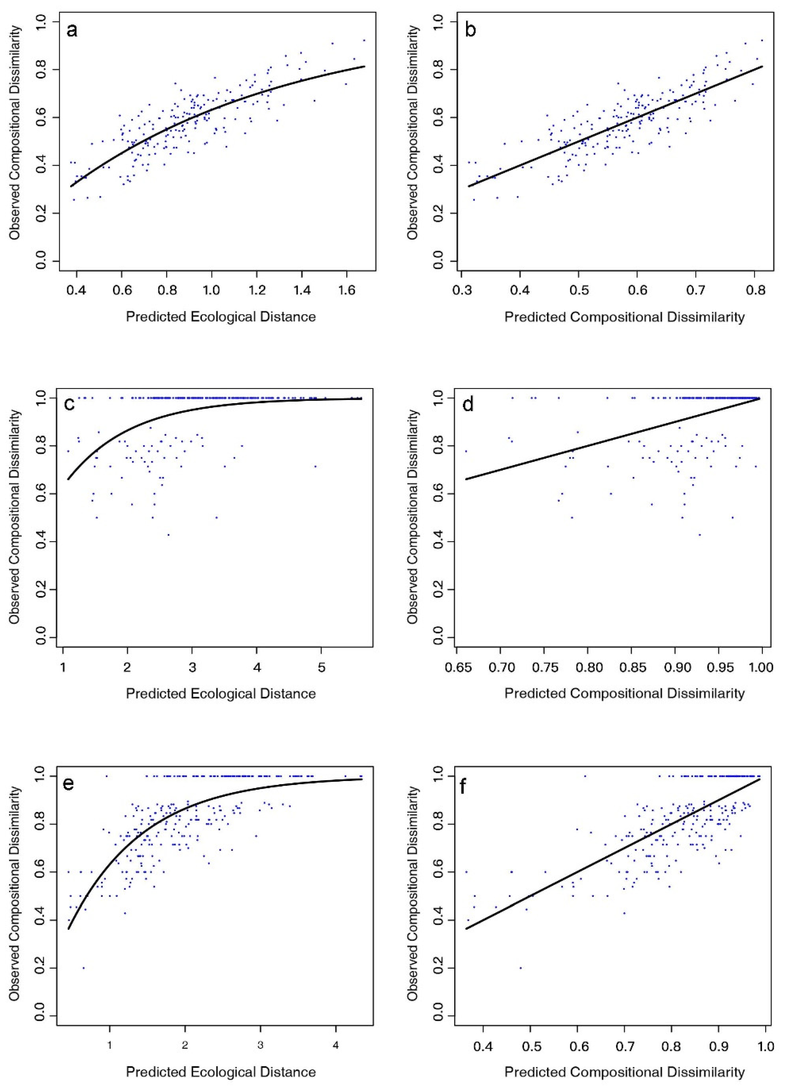
2.4. Multi-Site Generalized Dissimilarity Modeling (MS-GDM)

The MS-GDM model is an extension of the generalized linear model proposed by Ferrier et al. [30]. It can effectively solve the problems of curvilinar relationship between environmental dissimilarity at extreme values (0 or 1) and community composition dissimilarity. The model uses exponential functions to connect environmental data and Bray–Curtis dissimilarity data [30]. The MS-GDM model is defined as follows:
l n ( 1 d i j ) = b + k = 1 p | f k ( x k i ) f k ( x k j ) |
where i and j indicate different plots, dij is Bray–Curtis index, and b is fitted regression coefficient. k is environmental variables (k = 1, 2, …, p). xki and xkj are the observed values of environmental variable k in plots i and j. fk(xki)fk(xkj) provides the best possible fit between predicted and observed compositional dissimilarity. f k ( x k ) = k = 1 p a p k I p k ( x k ) , where apk is the fitted coefficient for Ipk, which is the kth I-spline for variable xk, and apk ≥ 0. In GDM, I-spline fits the hypothesis that composition differences between communities only increase with distance along environmental gradients
To avoid model overfitting, the length of fitted nodes (Knots) should be equal to the sum of spline vectors. The default three I-spline splines of minimum (0), median (50%), and maximum (100%) were used as spline piecewise fit nodes. The GDM approach implements automatic variable selection by using matrix permutation to verify the significance of the current model, adding or deleting environmental variables to subsequently evaluate the performance gains [30]. Then, GDM can output a Partial response graph, in which the maximum height of the curve represents the relative contribution of each environmental variable to β-diversity, and the slope of the curve represents the change rate of β-diversity following environmental gradients [31,32,33].
In addition to the use of GDM, the relationships between β-diversity components of trees, shrubs and herbs and each soil chemical properties in different soil depth layers were estimated using the Person correlation and Mantel test. The statistics, calculations and geographic mapping in this study were carried out using R software (version 4.1.0), involving packages such as “vegan”, “betapart” and “gdm” [30,33,34,35].

3. Results

3.1. β-Diversity Distribution Pattern of Different Plant Forms

A total of 233 species belonging to 132 genera and 70 families were found in plots, including 200 species of trees, 46 species of shrubs, and 68 species of herbs. By calculating the β-diversity index of different plant forms, we found that the βSOR of trees, shrubs, and herbs were 0.87, 0.95 and 0.94, respectively. This indicated that plant species composition differed greatly among plots in the study area, and the species compositional dissimilarity of shrubs and herbs was higher. After decomposition of β-diversity into its components (i.e., species turnover and nestedness), the species turnover was predominant in the three plant forms, while the nestedness accounted for less than 10%. This implied that the species turnover component is more important in species composition in the Nanling Mountains (Figure 2).
We found that species compositional dissimilarity of trees, shrubs, and herbs in the study area increased with distance, indicating that there was an obvious species turnover of plant community in the Nanling Mountains. Additionally, this was confirmed by the use of the GDM approach, since the predicted species compositional dissimilarity matched the observed species compositional dissimilarity of trees, shrubs, and herbs (Figure 3).

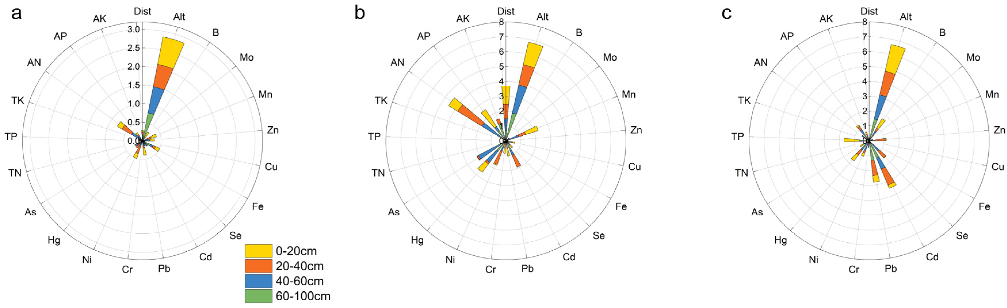
3.2. The Contribution of Environmental Factors to Plant β-Diversity by GDM

Soil chemical properties were the best explainers of tree β-diversity, with a mean explanation rate of 52.5%, followed by herbs (40.3%) and shrubs (21.8%) (Figure 4). With the increase in soil depth, the explanation rate of β-diversity of trees and herbs explained by soil chemical elements gradually decreased, since the explanation rate of chemical elements in the 0–20 cm soil layer remained consistently higher than the rates of deeper layers. Soil elements in the 60–100 cm layer showed the lowest explanatory power for β-diversity of trees, shrub and herbs.
Figure 5 shows the relationship between the species composition matrix and environment matrix fitted by I-spline function. The parameters of the spline function indicate the effects of altitude, geographic distance and soil chemical elements at different soil depths on the β-diversity of trees, shrubs and herbs. The β-diversity of trees was mainly affected by altitude and the element contents in the 0–60 cm soil layer, including AN (available nitrogen), Fe and Ni. In addition, the contents of Fe and Se in the 60–100 cm soil layer also showed important effects on tree β-diversity (Figures S1–S4). The β-diversity of shrubs was mainly determined by altitude, geographical distance and soil chemical elements in the 0–60 cm layer, including AN, AP, Cu and Hg in in the 0–20 cm layer, AN, Ni and Cd in the 20–40 cm layer, and An, As and Hg in the 40–60 cm layer. The chemical elements in the 60–100 cm soil layer showed little effect on the species composition of shrubs (Figures S5–S8). The β-diversity of herbs was mainly affected by altitude, B, Cd and Pb elements, with a stronger effect of the 0–40 cm layer on herb composition in comparison to deeper soil layers (Figures S9–S12).

3.3. Relationship between Soil Chemical Properties and β-Diversity of Different Plant Forms

The species turnover components of trees were positively correlated with TN, TP, AN, Cu and Hg at the 20–60 cm soil layer, and Cu and Hg at the 60–100 cm layer. The nestedness of trees was significantly correlated with the AP, Fe, Cr and Ni contents in the 0–60 cm soil layers. The species compositional dissimilarity of shrubs was significantly correlated with TN, TP, AN and Cu at the 0–60 cm soil layer, and the turnover component was significantly correlated with TN and AN. In the 0–20 cm topsoil layer, the turnover component of herbs was positively correlated with the contents of TP, Cd and Ni, while the nestedness component was negatively correlated with AP, Cd, and Ni of the 0–20 cm layer (Table 2, Table 3 and Table 4).

4. Discussion

4.1. The Predicted Contribution of Different Soil Depths to the β-Diversity of Nanling Forest Communities

Extensive studies on β-diversity of plant communities have helped to explain the mechanisms of community assemblage and diversity maintenance [6,36,37]. Through our study of Nanling ecosystems, it was found that plant species composition of three plant formations in the Nanling Mountains varies (mean βSOR 0.92) along different community types, and the species composition dissimilarity of shrubs and herbs was greater than that of trees. As a mountain ecosystem with a maximum altitude of only 1902m, the plant β-diversity patterns of the Nanling mountain are similar to that of alpine ecosystems in China [37,38]. β-diversity was decomposed into species turnover and species nestedness components, and the species turnover component was dominant, which was consistent with the research in other subtropical forests [38,39,40]. It is suggested that the β-diversity pattern of plant communities in the Nanling Mountains may be mainly caused by the species turnover or community development in different spaces. In addition, the dissimilarity of plant community species composition increased with the geographical distance. Significant spatial differences exist in the species composition of Nanling forest communities, suggesting that plant β-diversity patterns may be affected by dispersal constraints [40,41].
In this study, the GDM model showed 11, 9, 8, and 8 variables were related to the β-diversity of trees in 0–20 cm, 20–40 cm, 40–60 cm, and 60–100 cm soil depths, respectively. The soil element contents of 0–20 cm accounted for 63.5% of the β-diversity of trees. There were 7, 13, 5, and 5 variables significantly explaining the shrub β-diversity in 0–20 cm, 20–40 cm, 40–60 cm, and 60–100 cm depth soil layers, respectively, and 0–20 cm soil element contents were also the best explainers, up to 30.1% of the β-diversity. Regarding the herb β-diversity, there were 7, 10, 8, and 9 explainers in 0–20 cm, 20–40 cm, 40–60 cm and 60–100 cm soil layers, respectively. The 0–20 cm also had the highest explanatory ability, accounting for 45.5% of the herbs’ β-diversity. The distribution of trees (200 species) showed a more sensitive response to the soil element content heterogeneity than shrubs (46 species) and herbs (68 species). Previous studies suggested that GDM explained variation in species turnover for more widespread species, since, by definition, rare species are not shared by many sites [31,42]. We also speculate that the contribution of predictive variables fitted by GDM is closely related to the species pool in the study area, but further studies are needed to verify this [43].

4.2. Relative Effects of Environmental Filtration and Dispersal Limitation on the β-Diversity of Plant Communities

Many studies have confirmed that environmental filtration and dispersal limitation are important processes affecting species composition and community assemblage, but their relative roles in different ecosystems have not been generally concluded [6,44]. Based on GDM model, the species diversity of plant communities in Nanling showed a spatial increasing spatial pattern with the geographical distance. Environmental factors at different soil depths had different effects on the β-diversity of trees, shrubs, and herbs. This suggests that the environmental filtering process indicated by factors such as soil elements, and dispersal limitation characterized by geographical distance, both influenced the plant β-diversity and its components in the Nanling Mountains, which is consistent with previous studies in other mountains in southern China [38,40,45]. However, the relative contribution of environmental filtering and dispersal limitation on β-diversity in Nanling notably differs from the studies mentioned above, while according to our model, the dispersal limitation explained 8.78%, 16.64%, and 5.38% of the β-diversity of trees, shrubs, and herbs, while environmental factors such as altitude and soil explained significantly more. This seems to be indicative of ecosystem dynamics strongly driven by environmental heterogeneity [39,46], implying that in the Nanling Mountains ecosystems, environmental heterogeneity plays the dominant role in changes in species composition.

4.3. Effects of Environmental Factors on Different Components of β-Diversity

There are also some differences in the main factors affecting the species composition in different plant forms in Nanling. In this study, geographical distance showed a stronger effect on β-diversity components of shrubs than that of trees and herbs, which might be related to the heterogeneous dispersal ability of different plant forms. As an environmental factor reflecting the changes of water and heat conditions in mountain ecosystems, altitude usually has a significant correlation with species diversity [38,47]. In this study, altitude had a more important contribution to the species turnover components of tree and herb species, but a smaller influence on the β-diversity component of shrubs. Due to the nurse influence from trees, environment heterogeneity in the understory is low, so changes in precipitation, temperature and light radiation caused by altitude might have a lesser impact on the habitats of shrubs in the understory. Consequently, the shrubs considered in this study may not be markedly sensitive to altitude [38,48,49].
With the increase in soil depth, the effects of soil elements on the β-diversity of trees, shrubs, and herbs gradually decreased, which may be related to changes of the plant fine root amount with the increase of soil depth [50,51,52]. The active roots that plants can absorb nutrient elements and water through are mostly rootlets, and 50%–80% of the rootlets are located in the soil layer of 0–30 cm depth, and the root numbers decrease sharply after 30 cm depth [53,54]. The 0–60 cm depth soil was the main root distribution area of the tree species, strongly affected tree species composition. Available nitrogen in the 20–60 cm soil layer had a significant positive correlation with the turnover components of tree β-diversity, and available phosphorus in the 0–20 cm soil layer had a significant positive effect with the nested components of tree β-diversity. The shrub β-diversity and its turnover components were mainly related to the geographical distance between communities and were affected by soil factors of 0–40 cm depth soil, such as available nitrogen, phosphorus, potassium, and other nutrient elements. Soil nitrogen and phosphorus are essential nutrient elements for plant growth, which participate in various physiological processes of plant growth. However, the available phosphorus content in southern China’s soils is extremely low, which limits plant growth [22]. In this study area, the available phosphorus content in the 0–20 cm soil depth was relatively high (1.98 mg/kg on average), but decreased sharply below the 20 cm soil depth. The average available phosphorus content in the 20–40 cm soil layer was 0.84 C mg/kg. Therefore, phosphorus was the limiting resource for subtropical forest species’ growth.
The boron, iron, and copper content in the 0–20 cm soil layer had a significant positive effect on the β-diversity of trees, and copper in the 20–40 cm soil layer had a positive correlation with shrub β-diversity. Boron is involved in plant cell wall construction and affects plant metabolic pathways by binding apoplastic proteins of cell walls and membranes and by interfering with manganese-dependent enzymatic reactions [55]. Iron is essential for the structure of chloroplasts and mitochondria and for both plant productivity and nutritional quality [56,57]. Copper is a micronutrient which plays a role in processes such as photosynthesis, respiration, antioxidant activity, cell wall metabolism and hormone perception [58,59]. These three rare elements in the topsoil notably affect the tree species composition where the main rootlets of trees are distributed [60]. The chemical elements of 0–40 cm soil depth showed a stronger impact on the β-diversity of herbs, which may be related to the root of the herbaceous layer mainly concentrated in the topsoil [61]. Total nitrogen, total phosphorus, cadmium and nickel had significant positive correlations with β-diversity and turnover components of herbs, while the nested components were mainly negatively affected by available potassium, cadmium and nickel in the 0–20 cm topsoil. Heavy metals, such as cadmium and nickel, have been reported as phytotoxic at elevated concentrations, causing growth reduction, yield depression and disorder in plant metabolism and physiology [62,63].

5. Conclusions

This study provides three findings that might help to understand the species diversity maintenance mechanisms of different plant forms. First, the contribution of environmental factors and the dispersal process varied with plant forms, and soil factors had a stronger influence on the β-diversity of trees than that of shrubs and herbs. Secondly, with the increase of soil depth, the explanation rate of β-diversity of trees and herbs explained by soil chemical elements gradually decreased. Finally, the chemical elements of 0–60 cm soil mainly affected tree diversity, while the main soil factors affecting the β-diversity of shrubs and herbs were in 0–40 cm depth. We conclude that the deeper soil factors have broaden our understanding of influencing factors that shape plant communities. We suggest that models need to consider a broader spectrum of environmental factors that might affect plant community composition. We also suggest that the species composition and diversity patterns of the Nanling Mountains system need to be further studied.

Supplementary Materials

The following supporting information can be downloaded at: https://www.mdpi.com/article/10.3390/f13122184/s1, Figure S1: Partial response for 0–20 cm edaphic factors on trees’ GDM; Figure S2: Partial response for 20–40 cm edaphic factors on trees’ GDM; Figure S3: Partial response for 40–60 cm edaphic factors on trees’ GDM; Figure S4: Partial response for 60–100 cm edaphic factors on trees’ GDM; Figure S5: Partial response for 0–20 cm edaphic factors on shrubs’ GDM; Figure S6: Partial response for 20–40 cm edaphic factors on shrubs’ GDM; Figure S7: Partial response for 40–60 cm edaphic factors on shrubs’ GDM; Figure S8: Partial response for 60–100 cm edaphic factors on shrubs’ GDM; Figure S9: Partial response for 0–20 cm edaphic factors on herbs’ GDM; Figure S10: Partial response for 20–40 cm edaphic factors on herbs’ GDM; Figure S11: Partial response for 40–60 cm edaphic factors on herbs’ GDM; Figure S12: Partial response for 60–100 cm edaphic factors on herbs’ GDM; Table S1: Species composition and dominant species of different vegetation community at Nanling Mountains.

Author Contributions

Conceptualization, W.X. and P.Z.; methodology, Z.L.; validation, P.Y.; investigation, Z.T.; writing—review and editing, M.Á.G.-R.; project administration, P.Z. All authors have read and agreed to the published version of the manuscript.

Funding

This research was funded by the GDAS’ Special Project of Science and Development [2021GDASYL-20210103005], the Sub-project of National Key Research and Development projects [2021FY100702], Biodiversity maintenance mechanism and regional biosecurity innovation in Lingnan region [2022GDASZH-2022010106] and Ecosystem and Biodiversity Monitoring in Nanling National Park [LC-2021124].

Conflicts of Interest

The authors declare no conflict of interest.

References

  1. Rahbek, C. The role of spatial scale and the perception of large-scale species-richness patterns. Ecol. Lett. 2005, 8, 224–239. [Google Scholar] [CrossRef]
  2. Pollock, L.J.; O’Connor, L.M.J.; Mokany, K.; Rosauer, D.F.; Talluto, M.V.; Thuiller, W. Protecting Biodiversity (in All Its Complexity): New Models and Methods. Trends Ecol. Evol. 2020, 35, 1119–1128. [Google Scholar] [CrossRef] [PubMed]
  3. Magurran, A.E.; Dornelas, M.; Moyes, F.; Henderson, P.A. Temporal β diversity—A macroecological perspective. Glob. Ecol. Biogeogr. 2019, 28, 1949–1960. [Google Scholar] [CrossRef]
  4. Legendre, P.; De Cáceres, M. Beta diversity as the variance of community data: Dissimilarity coefficients and partitioning. Ecol. Lett. 2013, 16, 951–963. [Google Scholar] [CrossRef]
  5. Mori, A.S.; Isbell, F.; Seidl, R. Beta-Diversity, Community Assembly, and Ecosystem Functioning. Trends Ecol. Evol. 2018, 33, 549–564. [Google Scholar] [CrossRef]
  6. Qian, H.; Jin, Y.; Leprieur, F.; Wang, X.; Deng, T. Geographic patterns and environmental correlates of taxonomic and phylogenetic beta diversity for large-scale angiosperm assemblages in China. Ecography 2020, 43, 1706–1716. [Google Scholar] [CrossRef]
  7. Mori, A.S.; Shiono, T.; Koide, D.; Kitagawa, R.; Ota, A.T.; Mizumachi, E. Community assembly processes shape an altitudinal gradient of forest biodiversity. Glob. Ecol. Biogeogr. 2013, 22, 878–888. [Google Scholar] [CrossRef]
  8. Svenning, J.C.; Fløjgaard, C.; Baselga, A. Climate, history and neutrality as drivers of mammal beta diversity in Europe: Insights from multiscale deconstruction. J. Anim. Ecol. 2011, 80, 393–402. [Google Scholar] [CrossRef]
  9. König, C.; Weigelt, P.; Kreft, H. Dissecting global turnover in vascular plants. Glob. Ecol. Biogeogr. 2017, 26, 228–242. [Google Scholar] [CrossRef]
  10. Baselga, A. Partitioning the turnover and nestedness components of beta diversity. Glob. Ecol. Biogeogr. 2010, 19, 134–143. [Google Scholar] [CrossRef]
  11. Martins, P.M.; Poulin, R.; Goncalves-Souza, T. Drivers of parasite beta-diversity among anuran hosts depend on scale, realm and parasite group. Philos. T. R. Soc. B 2021, 376, 20200367. [Google Scholar] [CrossRef] [PubMed]
  12. Chase, J.M. Stochastic community assembly causes higher biodiversity in more productive environments. Science 2010, 328, 1388–1391. [Google Scholar] [CrossRef] [PubMed] [Green Version]
  13. Zhang, L.; Mi, X.; Harrison, R.D.; Yang, B.; Man, X.; Ren, H.; Ma, K. Resource Heterogeneity, Not Resource Quantity, Plays an Important Role in Determining Tree Species Diversity in Two Species-Rich Forests. Fron. Ecol. Evol. 2020, 8, 224. [Google Scholar] [CrossRef]
  14. Chesson, P. Mechanisms of maintenance of species diversity. Annu. Rev. Ecol. Syst. 2000, 31, 343–366. [Google Scholar] [CrossRef] [Green Version]
  15. Levine, J.M.; HilleRisLambers, J. The importance of niches for the maintenance of species diversity. Nature 2009, 461, 254–257. [Google Scholar] [CrossRef]
  16. Xue, W.; Bezemer, T.M.; Berendse, F. Soil heterogeneity and plant species diversity in experimental grassland communities: Contrasting effects of soil nutrients and pH at different spatial scales. Plant Soil. 2019, 442, 497–509. [Google Scholar] [CrossRef] [Green Version]
  17. Stein, A.; Gerstner, K.; Kreft, H. Environmental heterogeneity as a universal driver of species richness across taxa, biomes and spatial scales. Ecol. Lett. 2014, 17, 866–880. [Google Scholar] [CrossRef]
  18. Kallimanis, A.S.; Mazaris, A.D.; Tzanopoulos, J.; Halley, J.M.; Pantis, J.D.; Sgardelis, S.P. How does habitat diversity affect the species–area relationship? Glob. Ecol. Biogeogr. 2008, 17, 532–538. [Google Scholar] [CrossRef]
  19. Tukiainen, H.; Bailey, J.J.; Field, R.; Kangas, K.; Hjort, J. Combining geodiversity with climate and topography to account for threatened species richness. Conserv. Biol. 2017, 31, 364–375. [Google Scholar] [CrossRef]
  20. Bailey, J.J.; Boyd, D.S.; Field, R. Models of upland species’ distributions are improved by accounting for geodiversity. Landscape Ecol. 2018, 33, 2071–2087. [Google Scholar] [CrossRef]
  21. Hulshof, C.M.; Spasojevic, M.J. The edaphic control of plant diversity. Glob. Ecol. Biogeogr. 2020, 29, 1634–1650. [Google Scholar] [CrossRef]
  22. Zhang, L.; Mi, X.; Shao, H.; Ma, K. Strong plant-soil associations in a heterogeneous subtropical broad-leaved forest. Plant Soil 2011, 347, 211–220. [Google Scholar] [CrossRef]
  23. Hall, J.S.; McKenna, J.J.; Ashton, P.M.S.; Gregoire, T.G. Habitat characterizations underestimate the role of edaphic factors controlling the distribution of Entandrophragma. Ecology 2004, 85, 2171–2183. [Google Scholar] [CrossRef]
  24. Berendse, F. Competition between plant populations with different rooting depths. Oecologia 1979, 43, 19–26. [Google Scholar] [CrossRef]
  25. Bolte, A.; Villanueva, I. Interspecific competition impacts on the morphology and distribution of fine roots in European beech (Fagus sylvatica L.) and Norway spruce (Picea abies (L.) Karst.). Eur. J. Forest Res. 2006, 125, 15–26. [Google Scholar] [CrossRef]
  26. Brassard, B.W.; Chen, H.Y.; Cavard, X.; Laganiere, J.o.; Reich, P.B.; Bergeron, Y.; Pare, D.; Yuan, Z. Tree species diversity increases fine root productivity through increased soil volume filling. J. Ecol. 2013, 101, 210–219. [Google Scholar] [CrossRef]
  27. Jackson, R.B.; Canadell, J.; Ehleringer, J.R.; Mooney, H.; Sala, O.; Schulze, E.-D. A global analysis of root distributions for terrestrial biomes. Oecologia 1996, 108, 389–411. [Google Scholar] [CrossRef]
  28. Nanjing Institute of Soil Science. Analysis of Soil Physical and Chemical Properties; Shanghai Science and Technology Publishing House: Shanghai, China, 1978. [Google Scholar]
  29. Team, R.C. R: A Language and Environment for Statistical Computing; R Foundation for Statistical Computing: Vienna, Austria, 2021. [Google Scholar]
  30. Ferrier, S.; Manion, G.; Elith, J.; Richardson, K. Using generalized dissimilarity modelling to analyse and predict patterns of beta diversity in regional biodiversity assessment. Divers. Distrib. 2007, 13, 252–264. [Google Scholar] [CrossRef]
  31. Overton, J.M.; Barker, G.M.; Price, R. Estimating and conserving patterns of invertebrate diversity: A test case of New Zealand land snails. Divers. Distrib. 2009, 15, 731–741. [Google Scholar] [CrossRef]
  32. Ashcroft, M.B.; Gollan, J.R.; Faith, D.P.; Carter, G.A.; Lassau, S.A.; Ginn, S.G.; Bulbert, M.W.; Cassis, G. Using generalised dissimilarity models and many small samples to improve the efficiency of regional and landscape scale invertebrate sampling. Ecol. Inform. 2010, 5, 124–132. [Google Scholar] [CrossRef]
  33. Leaper, R.; Hill, N.A.; Edgar, G.J.; Ellis, N.; Lawrence, E.; Pitcher, C.R.; Barrett, N.S.; Thomson, R. Predictions of beta diversity for reef macroalgae across southeastern Australia. Ecosphere 2011, 2, 1–18. [Google Scholar] [CrossRef]
  34. Oksanen, J.; Simpson, G.L.; Blanchet, F.G.; Kindt, R.; Legendre, P.; Minchin, P.R.; O’Hara, R.B.; Solymos, P.; Stevens, M.H.H.; Eduard, S.; et al. Package ‘vegan’. Community Ecology Package; R Package Version 2.6-4; R Foundation for Statistical Computing: Vienna, Austria, 2022. [Google Scholar]
  35. Baselga, A.; Orme, D.; Villeger, S.; Bortoli, J.D.; Leprieur, F.; Logez, M. betapart: Partitioning Beta Diversity into Turnover and Nestedness Components, R package Version 1.5.6; R Foundation for Statistical Computing: Vienna, Austria, 2022. [Google Scholar]
  36. Zellweger, F.; Roth, T.; Bugmann, H.; Bollmann, K. Beta diversity of plants, birds and butterflies is closely associated with climate and habitat structure. Glob. Ecol. Biogeogr. 2017, 26, 898–906. [Google Scholar] [CrossRef]
  37. Nanda, S.A.; Haq, M.-u.; Singh, S.; Reshi, Z.A.; Rawal, R.S.; Kumar, D.; Bisht, K.; Upadhyay, S.; Upreti, D.; Pandey, A. Species richness and β-diversity patterns of macrolichens along elevation gradients across the Himalayan Arc. Sci. Rep. 2021, 11, 20155. [Google Scholar] [CrossRef] [PubMed]
  38. Tang, Z.; Fang, J.; Chi, X.; Feng, J.; Liu, Y.; Shen, Z.; Wang, X.; Wang, Z.; Wu, X.; Zheng, C. Patterns of plant beta-diversity along elevational and latitudinal gradients in mountain forests of China. Ecography 2012, 35, 1083–1091. [Google Scholar] [CrossRef]
  39. Kouba, Y.; Martínez-García, F.; de Frutos, Á.; Alados, C.L. Plant β-diversity in human-altered forest ecosystems: The importance of the structural, spatial, and topographical characteristics of stands in patterning plant species assemblages. Eur. J. Forest Res. 2014, 133, 1057–1072. [Google Scholar] [CrossRef] [Green Version]
  40. Shi, W.; Wang, Y.Q.; Xiang, W.S.; Li, X.K.; Cao, K.F. Environmental filtering and dispersal limitation jointly shaped the taxonomic and phylogenetic beta diversity of natural forests in southern China. Ecol. Evol. 2021, 11, 8783–8794. [Google Scholar] [CrossRef] [PubMed]
  41. Jiang, L.; Lv, G.; Gong, Y.; Li, Y.; Wang, H.; Wu, D. Characteristics and driving mechanisms of species beta diversity in desert plant communities. PLoS ONE 2021, 16, e0245249. [Google Scholar] [CrossRef] [PubMed]
  42. Latombe, G.; Hui, C.; McGeoch, M.A. Multi-site generalised dissimilarity modelling: Using zeta diversity to differentiate drivers of turnover in rare and widespread species. Methods Ecol. Evol. 2017, 8, 431–442. [Google Scholar] [CrossRef] [Green Version]
  43. Krasnov, B.R.; Shenbrot, G.I.; Vinarski, M.M.; Korallo-Vinarskaya, N.P.; Khokhlova, I.S.; McGeoch, M. Multi-site generalized dissimilarity modelling reveals drivers of species turnover in ectoparasite assemblages of small mammals across the northern and central Palaearctic. Glob. Ecol. Biogeogr. 2020, 29, 1579–1594. [Google Scholar] [CrossRef]
  44. Myers, J.A.; Chase, J.M.; Jiménez, I.; Jørgensen, P.M.; Araujo-Murakami, A.; Paniagua-Zambrana, N.; Seidel, R. Beta-diversity in temperate and tropical forests reflects dissimilar mechanisms of community assembly. Ecol. Lett. 2013, 16, 151–157. [Google Scholar] [CrossRef]
  45. Legendre, P.; Mi, X.; Ren, H.; Ma, K.; Yu, M.; Sun, I.-F.; He, F. Partitioning beta diversity in a subtropical broad-leaved forest of China. Ecology 2009, 90, 663–674. [Google Scholar] [CrossRef] [PubMed] [Green Version]
  46. Jankowski, J.E.; Ciecka, A.L.; Meyer, N.Y.; Rabenold, K.N. Beta diversity along environmental gradients: Implications of habitat specialization in tropical montane landscapes. J. Anim. Ecol. 2009, 78, 315–327. [Google Scholar] [CrossRef] [PubMed]
  47. Ficetola, G.F.; Mazel, F.; Thuiller, W. Global determinants of zoogeographical boundaries. Nat. Ecol. Evol. 2017, 1, 1–7. [Google Scholar] [CrossRef] [PubMed]
  48. Barnes, P.W.; Archer, S. Influence of an overstorey tree (Prosopis glandulosa) on associated shrubs in a savanna parkland: Implications for patch dynamics. Oecologia 1996, 105, 493–500. [Google Scholar] [CrossRef] [PubMed]
  49. Wang, J.; Wang, Y.; Li, M.; He, N.; Li, J. Divergent roles of environmental and spatial factors in shaping plant β-diversity of different growth forms in drylands. Glob. Ecol. Conserv. 2021, 26, e01487. [Google Scholar] [CrossRef]
  50. Wang, Y.; Dong, X.; Wang, H.; Wang, Z.; Gu, J. Root tip morphology, anatomy, chemistry and potential hydraulic conductivity vary with soil depth in three temperate hardwood species. Tree Physiol. 2016, 36, 99–108. [Google Scholar] [CrossRef] [Green Version]
  51. Maeght, J.-L.; Gonkhamdee, S.; Clement, C.; Isarangkool Na Ayutthaya, S.; Stokes, A.; Pierret, A. Seasonal patterns of fine root production and turnover in a mature rubber tree (Hevea brasiliensis Müll. Arg.) stand-differentiation with soil depth and implications for soil carbon stocks. Front. Plant Sci. 2015, 6, 1022. [Google Scholar] [CrossRef] [Green Version]
  52. Schwinning, S.; Litvak, M.; Pockman, W.; Pangle, R.; Fox, A.; Huang, C.-W.; McIntire, C. A 3-dimensional model of Pinus edulis and Juniperus monosperma root distributions in New Mexico: Implications for soil water dynamics. Plant Soil 2020, 450, 337–355. [Google Scholar] [CrossRef]
  53. Krišāns, O.; Samariks, V.; Donis, J.; Jansons, Ā. Structural Root-plate characteristics of wind-thrown Norway spruce in hemiboreal forests of Latvia. Forests 2020, 11, 1143. [Google Scholar] [CrossRef]
  54. Awé, D.V.; Noiha, N.V.; Vroh, B.T.A.; Zapfack, L. Root Distribution of Four Tree Species Planted in Living Hedges according to Two Types of Soil and Three Agroforestry Technologies in the Sudano-Sahelian Zone of Cameroon. Open J. Agric. Res. 2021, 1, 74–83. [Google Scholar]
  55. Blevins, D.G.; Lukaszewski, K.M. Boron in plant structure and function. Annu. Rev. Plant Biol. 1998, 49, 481–500. [Google Scholar] [CrossRef] [PubMed]
  56. Briat, J.-F.; Duc, C.; Ravet, K.; Gaymard, F. Ferritins and iron storage in plants. BBA–Gen. Subj. 2010, 1800, 806–814. [Google Scholar] [CrossRef] [PubMed]
  57. López-Millán, A.F.; Duy, D.; Philippar, K. Chloroplast iron transport proteins–function and impact on plant physiology. Front. Plant sci. 2016, 7, 178. [Google Scholar] [CrossRef] [PubMed] [Green Version]
  58. Pilon, M.; Abdel-Ghany, S.E.; Cohu, C.M.; Gogolin, K.A.; Ye, H. Copper cofactor delivery in plant cells. Curr. Opin. Plant biol. 2006, 9, 256–263. [Google Scholar] [CrossRef] [PubMed]
  59. Yruela, I. Copper in plants: Acquisition, transport and interactions. Funct. Plant Biol. 2009, 36, 409–430. [Google Scholar] [CrossRef] [PubMed] [Green Version]
  60. Schenk, H.J.; Jackson, R.B. The global biogeography of roots. Ecol. Monogr. 2002, 72, 311–328. [Google Scholar] [CrossRef]
  61. Li, J.; He, B.; Chen, Y.; Huang, R.; Tao, J.; Tian, T. Root distribution features of typical herb plants for slope protection and their effects on soil shear strength. TCSAE 2013, 29, 144–152. [Google Scholar]
  62. Sheoran, I.; Aggarwal, N.; Singh, R. Effects of cadmium and nickel on in vivo carbon dioxide exchange rate of pigeon pea (Cajanus cajan L.). Plant Soil 1990, 129, 243–249. [Google Scholar] [CrossRef]
  63. Papazoglou, E.G.; Serelis, K.G.; Bouranis, D.L. Impact of high cadmium and nickel soil concentration on selected physiological parameters of Arundo donax L. Eur. J. Soil Biol. 2007, 43, 207–215. [Google Scholar] [CrossRef]
Figure 1. Geographical locations of the study area.
Forests 13 02184 g001
Figure 2. β-diversity and components of different plant forms of the Nanling Mountains.
Forests 13 02184 g002
Figure 3. Relationships between compositional dissimilarity and geographical distance and relationships between predicted species compositional dissimilarity and the observed species compositional dissimilarity of different life form plants ((a,b) indicate trees, (c,d) indicate shrubs, (e,f) indicate herbs).
Forests 13 02184 g003
Figure 4. Contribution of environmental factors to plant β-diversity at different soil depths.
Forests 13 02184 g004
Figure 5. Sum of I-spline coefficients for environmental factors on β-diversity of trees (a), shrubs (b) and herbs (c). environmental factors included geographical distance (Dist), altitude (Alt), Boron (B), Molybdenum (Mo), Manganese (Mn), Zinc (Zn), Cuprum (Cu), Ferrum (Fe), Selenium (Se), Cadmium (Cd), Plumbum (Pb), Chromium (Cr), Nickel (Ni), Hydrargyrum (Hg) and Arsenic (As), Total nitrogen (TN), Total phosphorus (TP), Total kalium (TK) and Available nitrogen (AN), Available phosphorus (AP), Available kalium (AK).
Forests 13 02184 g005
Table 1. Elemental contents in different soil depths.
Element ContentsSoil Depths (cm)F-Valuep-Value
0–2020–4040–6060–100
B(mg/kg)23.72(±1.8)27.40(±2.0)27.92(±2.0)27.35(±2.1)9.19<0.0001 ***
Mo(mg/kg)3.85(±1.1)4.24(±1.2)4.20(±1.0)4.43(±1.2)2.230.0919
Mn(mg/kg)139.15(±13.1)155.46(±17.0)196.49(±23.2)244.63(±44.2)7.340.0002
Zn(mg/kg)61.92(±2.9)80.71(±10.4)72.79(±2.4)81.19(±4.4)2.410.0743
Cu(mg/kg)6.76(±0.8)5.87(±0.7)6.43(±0.7)6.71(±0.9)4.920.0037 **
Fe(mg/kg)23.03(±1.6)26.53(±1.8)26.43(±1.6)26.06(±1.8)9.64<0.0001 ***
Se(mg/kg)1.45(±0.1)1.39(±0.1)1.16(±0.1)0.93(±0.1)27.55<0.0001 ***
Cd(mg/kg)0.19(±0.01)0.09(±0.01)0.07(±0.01)0.07(±0.01)70.40<0.0001 ***
Pb(mg/kg)78.25(±4.3)94.88(±10.0)90.55(±7.8)106.05(±16.5)2.160.1008
Cr(mg/kg)26.86(±1.8)45.21(±2.9)52.88(±3.5)51.85(±4.8)16.03<0.0001 ***
Ni(mg/kg)10.43(±0.7)21.56(±2.1)25.47(±2.1)27.81(±2.8)24.34<0.0001 ***
Hg(mg/kg)0.35(±0.02)0.33(±0.02)0.31(±0.02)0.27(±0.01)10.70<0.0001 ***
As(mg/kg)20.11(±1.2)20.87(±1.6)20.25(±1.4)20.56(±1.7)0.590.6237
TN(g/kg)3.35(±0.2)2.42(±0.3)1.87(±0.3)1.38(±0.2)41.26<0.0001 ***
TP(g/kg)0.24(±0.02)0.25(±0.02)0.23(±0.02)0.19(±0.02)11.17<0.0001 ***
TK(g/kg)22.27(±1.1)29.78(±1.3)31.28(±1.1)32.55(±1.4)73.28<0.0001 ***
AN(mg/kg)246.39(±15.8)264.39(±27.1)205.83(±28.7)150.79(±21.2)17.77<0.0001 ***
AP(mg/kg)1.98(±0.2)0.84(±0.2)0.58(±0.2)0.31(±0.1)24.10<0.0001 ***
AK(mg/kg)80.04(±4.8)109.88(±7.0)101.95(±7.2)110.56(±10.3)10.59<0.0001 ***
Notes: p-value < 0.001, ***; p-value < 0.01, **.
Table 2. The coefficients of Pearson correlation between β-diversity components of trees and soil factors of different depths.
Soil Propertiesβ-sorβ-simβ-nes
0–20 cm20–40 cm40–60 cm60–100 cm0–20 cm20–40 cm40–60 cm60–100 cm0–20 cm20–40 cm40–60 cm60–100 cm
TN0.010.09 **0.11 *0.12−0.00020.090.09 **0.000.001−0.08−0.23−0.01
TP0.060.04 *0.03 *0.07 *0.010.03 *0.020.020.000.000.0020.00
TK0.020.02−0.0010.020.010.01−0.0040.010.0010.000.01−0.01
AN0.010.12 **0.13 **0.0030.010.11 **0.1 **0.01−0.0010.00−0.0002−0.01
AP−0.0040.040.060.002−0.020.010.050.000.05 *0.020.001−0.01
AK0.031 *−0.00010.030.020.05 *0.0030.05 *0.05−0.02−0.03−0.03−0.04
B0.05 *0.02−0.0020.000.010.01−0.010.000.030.010.030.01
Cu0.07 **0.08 **0.09 **0.07 *0.06 *0.06 *0.06 *0.04 *0.000.000.000.01
Fe0.05 *0.03 *0.000.010.010.01−0.01−0.0010.05 *0.020.08 **0.07
Se0.03 *−0.00040.002−0.010.05 *0.0010.001−0.003−0.02−0.010.00−0.001
Cd0.004−0.004−0.040.000.01−0.001−0.010.01−0.02−0.01−0.01−0.01
Cr0.001−0.0020.0002−0.02−0.01−0.01−0.01−0.010.06 *0.010.03−0.001
Ni0.0030.010.004−0.01−0.010.001−0.003−0.010.1 **0.040.08 *0.00
Hg0.010.08 ***0.10 **0.04 *0.020.09 ***0.13 **0.04 *−0.03−0.01−0.03−0.004
Notes: p-value < 0.001, ***; p-value < 0.01, **; p-value < 0.05, *.
Table 3. The coefficients of Pearson correlation and Mantel test between β-diversity components of shrubs and soil factors of different depths.
Soil Propertiesβ-sorβ-simβ-nes
0–20 cm20–40 cm40–60 cm60–100 cm0–20 cm20–40 cm40–60 cm60–100 cm0–20 cm20–40 cm40–60 cm60–100 cm
TN0.0050.02 *0.02 *0.00040.010.02 *0.02 *0.15−0.55−0.01−0.01−0.002
TP0.0020.02 *0.010.0010.0010.010.010.0080.002−0.003−0.01−0.0003
TK0.002−0.002−0.010-.010.001−0.003−0.028−0.020.00010.0040.020.01
AN0.02 *0.04 **0.030.0010.020.03 *0.03 *0.001−0.01−0.01−0.01−0.001
AP0.010.0040.020.0020.010.010.020.002−0.003−0.005−0.01−0.001
AK−0.13−0.0020.010.0010.0010.0020.0040.001−0.003−0.002−0.0020.001
B−0.002−0.0003−0.01−0.01−0.001−0.002−0.02−0.020.00010.0040.010.02
Cu0.020.03 *0.030.030.010.010.010.010.0010.0006−0.0001−0.0004
Fe0.00010.0001−0.004−0.010.001−0.001−0.01−0.01−0.0020.00060.010.01
Se0.01−0.030.002−0.010.0003−0.0020.001−0.020.0030.01−0.030.01
Cd0.0030.01−0.0020.0040.00010.004−0.001−0.010.002−0.002−0.0020.004
Cr0.0010.02−0.004−0.003−0.0010.010.001−0.0010.004−0.006−0.01−0.002
Ni0.010.030.0010.00010.0020.020.0030.0020.0001−0.001−0.01−0.01
Hg−0.010.0030.020.01−0.0010.00020.010.020.0010.0010.001−0.02
Notes: p-value < 0.01, **; p-value < 0.05, *.
Table 4. The coefficients of Pearson correlation and Mantel test between β-diversity components of herbs and soil factors of different depths.
Soil Propertiesβ-sorβ-simβ-nes
0–20 cm20–40 cm40–60 cm60–100 cm0–20 cm20–40 cm40–60 cm60–100 cm0–20 cm20–40 cm40–60 cm60–100 cm
TN0.690.04 *0.01−0.130.010.0130.0020.002−0.280.650.010.003
TP0.14 **0.020.0010.050.06 **0.0100.02 *−0.12−0.030.002−0.01
TK0.16−0.003−0.020.10−0.04−0.001−0.01−0.00010.0002−0.0010−0.001
AN0.03 *0.04 *0.020.070.010.010.00200.0010.010.010
AP−0.340.0020.001−0.14−0.0100.020.010.020.010.0020.02
AK0.010.010.030.010.020.010.030.02−0.03 *−0.002−0.01−0.01
B0.03 *0.04 *0.010.04 *0.030.05 *0.020.05 **−0.02−0.03−0.02−0.03 *
Cu0.020.020.020.010.0010.0020.00200.020.020.020.02
Fe0.020.020.010.020.020.03 *0.010.03 *−0.01−0.02−0.004−0.01
Se0.020.00040.010.010.010.0010.0030.010.002−0.1−0.001−0.01
Cd0.15 ***0.020.010.010.13 ***0.010.010.02−0.04 *−0.009−0.001−0.01
Cr−0.00020.03−0.0030.002−0.010.04−0.0004−0.0030.02−0.02−0.001−0.004
Ni0.08 **0.12 **0.03 *0.020.09 **0.11 **0.030.03−0.05 **−0.03−0.02−0.02
Hg0.010.06 **0.05 **0.020.010.05 **0.0020.004−0.0004−0.010.09 **0.01
Notes: p-value < 0.001, ***; p-value < 0.01, **; p-value < 0.05, *.
Publisher’s Note: MDPI stays neutral with regard to jurisdictional claims in published maps and institutional affiliations.

