Optimizing Operational-Level Forest Biomass Logistic Costs for Storage, Chipping and Transportation through Roadside Drying

Abstract

Forest biomass (FB) could supply more of Australia’s energy needs, but delivered costs must be reduced for it to be a viable energy source. Operational planning is critical to reducing delivered costs as it determines actual activities, though few operational FB supply chain (FBSC) planning tools have been published. This paper presents a “proof-of-concept” operational FBSC decision support system (DSS) to schedule FB deliveries for eight weeks from roadside storage for the least cost, taking in account moisture content changes. Four mathematical models are compared, solving a linear formulation of the FB delivery problem in terms of solution speed and delivered cost, and the practicality of implementing the solutions. The best performing model was a Greedy algorithm as it produced solutions not significantly different from those of the tested linear programming solver and was readily modified to significantly improve solution implementation through the addition of a non-linear element. FBSC planning tools typically assume accurate knowledge of stored FB quantities and that little or no rainfall occurs during storage. In practice, stored FB quantity estimates can be inaccurate due to variation in the bulk density of the piles. Improving these estimates is a critical area for future research. This study found that simulated rainfall with <20 mm during the first week of the scheduled period did not significantly effect delivered costs.

1. Introduction

Demand for biofuels is rising as a means to reduce global greenhouse gas emissions. Forest biomass (FB) (defined as any tree component or the whole tree), particularly logging residue (LR) [1], could potentially supply a major part of the energy needs of many countries, including Australia [2]. Industrial-scale use of FB for biofuel is an emerging industry in Australia, where it currently supplies less than 2% of the country’s energy needs [3]. Current Australian FB harvesting for biofuel is mainly ad hoc and opportunistic, providing considerable opportunities for improvements and cost reduction.

A plethora of FBSC planning models have been published, with [4,5,6] collectively reviewing over 60 published FBSC models, the majority of which dealt with strategic and tactical planning problems. D’Amours et al. [7] noted that “operational planning is really the planning process that fixes how and when the value will be captured”. In spite of this, a very limited number of operational level FBSC planning models have been published [8], the majority of which deal with transport scheduling and routing, for example, [9] and [10].

The development of new FBSC models has been accompanied by the development or adoption by forest researchers of methods to solve forest planning problems that can be broadly classified as optimization or heuristic methods. Bettinger et al. [11] noted that, whereas optimization methods give the optimal solution, the downside is that some complex relationships cannot be formulated as linear or mixed integer equations and that some problems cannot be solved in a reasonable time period. In contrast, the nearness of the heuristic solution to the optimum (the solution quality) is not always known but the solving speed of heuristics and their ability to solve otherwise intractable problems has led to increasing development in this area [11].

Evaluating the performance of published forest planning models has generally been performed through comparisons with existing models in terms of predicted cost or other economic measures, and solution times, e.g., [12,13,14,15,16]. As operational forest planning models produce solutions that users would expect to be implementable with little or no modification, the performance of these models needs to also evaluate the practicality of implementing solutions, though this is often not explicitly considered.

FB is characterized by high moisture content (MC) and low bulk, spatial and energy densities, and low value relative to fossil fuel sources [17]. FBSC are often complex, with multiple sources and destinations, and spatial and temporal variations in supply quantity and quality [5]. As a consequence, FB delivered costs are typically higher than those of other fuel sources, inhibiting its widespread use [4]. As transport costs are a major component of delivered FB costs (up to 50%) [18], transport cost savings are critical to reducing FB delivered costs. This was aptly summarized by [19], who stated “optimizing forest-fuel production essentially means minimizing transport costs”. This is particularly true for LR due to its very low bulk density when uncomminuted (~100 kg/m³ for fresh Eucalyptus nitens (H.Deane & Maiden) Maiden LR (unpublished data)) and high MC (typically >50% on a wet weight basis (e.g., [20,21])). Roadside drying and comminution prior to secondary transport can increase LR’s bulk density and net calorific value [22,23,24]. Despite this, few FBSC models include drying infield or at roadside prior to transport, and of these, few use drying models to predict the MC of stored FB [25]. An example of an FBSC model using a drying model to predict FB MC is the WAFFS model developed by [26], which allows users to simulate various forest fuel supply chain scenarios.

The short planning horizon at an operational level can make operational plans vulnerable to disruption by natural events, machinery breakdowns, etc. Disruptions to transport schedules in particular have to be dealt with in real-time, which is a challenge for a transport scheduling DSS [10,27]. The longer planning horizons associated with coupe scheduling (typically weekly) makes them more resilient to short-term disruptions. In the case of scheduling operations related to FB stored at roadside, precipitation is a major potential source of disruptions due to the effects on road access and FB MC [28,29]. The risk to FB MC is mitigated in Europe by covering roadside FB piles [30]; however, in Australia there is no experience with covering roadside FB and skepticism about its value under Australian weather conditions. Predictions of rainfall quantity up to 7 days in advance are currently used by forest managers to plan for potential impacts on field operations. However, the impact on the MC of stored FB and hence on delivery schedules in Australia is uncertain.

The objective of this paper is to develop a “proof-of-concept” operational DSS to assist forest managers in making optimal or near-optimal chipping and transport decisions for FB stored at roadside to meet customer weekly energy requirements for the lowest delivered cost, taking into account the transport distance, road type, and modelled changes in FB MC based on weather conditions. The impact of simulated rainfall in the first week of storage on the FB delivery schedule was also investigated.

2. Materials and Methods

2.1. Problem Description

The scope of the DSS in the current study within the context of an FBSC is shown in Figure 1. The DSS was designed to assist planners in delivering FB stored at roadside at harvest sites for the lowest cost while meeting weekly customer energy demand over an eight-week period. Delivered costs include chipping, and primary and secondary transport costs. Chipping was performed by mobile chippers such as the Petersen 4310B Tracked Chipper (Eugene, OR, USA) directly into trucks. These chippers require an excavator for loading. Dry matter losses consisted of a fixed component to account for retention of the contaminated bottom layer of the pile and a variable component related to handling and chipping that increased with decreasing pile MC, which was based on the findings of [31,32]. Other storage costs [33] and material losses were excluded as [34] reported that their impact on FB delivered costs for short storage periods (≤two months) was negligible.

Primary transport costs were based on the quantity of LR transported and the type of roundwood harvest (whole tree to roadside, fuel-adapted harvest, or cut-to-length at the stump), which set the transport cost (AUD/t) (

Table 1. Operational DSS input variables ¹.

Input Variable	Units	Range/Value	Comment
FB quantity	Tonnes	≤5000	Green weight
FB start date	Date	≥1 month before today	Date forest biomass was extracted to roadside
FB pile location	Coordinates
Distance	kilometre	1–150	Road distance from each FB pile to each customer
Proportion of distance on tracks	%	≤100	Cost increased by 20% for proportion of road distance travelled on tracks (Source: [35])
Energy requirement	GJ/week	≤20,000	Customer energy requirement for each week in the planning period
Bulk density (chips) (0% MC) (weight/bulk volume)	kg/m3	189
Energy content at 0% MC	GJ/t	18–22	Source: [36]
Chipping cost 2	AUD/t		Chipping costs increase with decreasing MC to reflect increased chipper wear and tear. Source: [24].
>50%		9.5
36–50%		9.7
<36%		10
Primary transport cost	AUD/t	0	Whole tree to roadside
		13	Cut to length at the stump
		9.4	Fuel-adapted harvest
			Source: [37]
Secondary transport cost	AUD/t-km		Source: [34]
1–25 km		0.20
25–50 km		0.15
50–75 km		0.15
75–100 km		0.14
100–125 km		0.13
125–150 km		0.12

¹ All dollar values are expressed in Australian dollars. ² Chipper costs are also a function of secondary transport distance; however, [38] found that, if three trucks serviced one chipper, costs were relatively consistent for the transport distance range modelled in the current DSS.

). Secondary transport costs were calculated by multiplying a transport charge in terms of dollars per tonne-kilometre (Table 1) with the distance from the harvest site to the customer and the weight of material transported. Total FB supply was constrained by user-defined initial weight of FB (wet basis) at each harvest site.

Inputs for the DSS in the current study are listed in Table 1. FB quantity, start date, pile location, distance, and proportion of distance on tracks were extracted from the forest management organization’s GIS database. Customer weekly energy requirements were entered into the DSS by the user. For the proof-of-concept DSS, only two customers and ten sites were modelled and only one truck type could be assigned to each harvest site/customer combination. Two truck types were modelled: a “standard” semi-trailer (26.5 t load weight, 75 m³ volumetric capacity) and a high-volumetric capacity semi-trailer (26 t load weight, 100 m³ volumetric capacity) [24]. In the current study, only E. nitens LR was modelled.

2.2. DSS Outputs

• The outputs from the DSS were as follows: Weekly quantity of FB chipped and transported from each harvest site to each customer.
• Number and location (site) of chippers required each week.
• Number of truckloads of residue delivered each week to each customer

2.3. FB MC and Net Calorific Value

Each time the DSS was ran, the MC of each FB pile at the current day was calculated using meteorological data obtained from the nearest Bureau of Meteorology (BOM) weather station and a published E. nitens LR drying model [39]. Initial pile MC was assumed to be that of fresh E. nitens LR (53%). From the current day onward, the weekly MC of each LR pile was determined using a modified version of the published E. nitens LR drying model with the rain response removed (Figure 2).

The DSS calculated FB net calorific value at MC (wet basis) as follows [40]:

$$NC{V}_{MC}=NC{V}_{0\%}\times \left(\frac{100-MC}{100}\right)-0.02443\times MC$$

where NCV_MC is the net calorific value (at constant pressure) at a given MC (%) (MJ/kg), NCV_0% is the net calorific value (at constant pressure) at 0% MC (MJ/kg), MC is MC as received (wet weight %), and 0.02443 is the correction factor of the enthalpy of vaporization (constant pressure) for water (moisture) at 25 °C (in MJ/kg per 1% MC).

2.4. Mathematical Model

The performances of the four mathematical models were compared to select the most appropriate model for the current operational FBSC DSS. The problem was formulated using linear constraints and the objective function to allow a linear programming (LP) solver to be compared with the three heuristic algorithms. The heuristic algorithms tested were the two supplied with MS Excel (the GRG (Generalized Reduced Gradient) non-linear and Evolutionary algorithms) and a Greedy algorithm coded by the principal author in Visual Basic for Applications (VBA). To reduce the chance of the GRG algorithm stopping at a local minimum, the “multi-start” option was used, which triggers the solver to perform multiple runs and to find the best solution. These mathematical models were selected as they cover a range of model types and are readily available to potential DSS users, most of whom are likely to have MS Excel installed on their computer. Use of third-party solvers was avoided to decrease updating requirements and cost (if commercial solvers were used).

The notation used in the model is shown in

Table 2. Notation used in the model.

Term	Definition
	Sets
i	Periods, i ∈ I = {1…8}
s	Supply areas, s ∈ S = {1…10}
c	Customers c ∈ C = {1,2}
	Parameters
SCRWs	Weight of forest biomass available in supply area s (t) (at maximum MC)
DTFBcs	Distance between supply area s and customer c (km)
EDic	Energy demand of customer c in period i (energy unit, MWh)
ECFBis	Energy content of chips produced in supply area s and period i from forest biomass stacked at the roadside (energy unit per tonne of chips, MWh/t)
CPFBcs	Primary transport cost for forest biomass moved to roadside in supply area s and delivered to customer c (AUD/t)
CSFBcs	Secondary transport cost for forest biomass stacked at the roadside in supply area s and delivered to customer c (AUD/t-km)
CCFBis	Chipping cost for forest biomass stacked at roadside in supply area s and period i (AUD/t)
	Variables
Xics	Weight of forest biomass chipped and transported in period i, for customer c in supply area s (t) (at maximum MC)
X’ics	Weight of chips produced from forest biomass chipped and transported in period i, for customer c, in supply area s, adjusted for MC changes during storage (t)

.

Objective function (Equation (1)).

$$Min={\displaystyle \sum }_i{\displaystyle \sum }_c{\displaystyle \sum }_s{X^{\prime }}_{ics}\times \left(CPF{B}_{cs}+(CSF{B}_{cs}\times DTF{B}_{cs}\right)+CCF{B}_{is})$$

(1)

Equation (2) ensures that the availability of forest biomass in each supply area is not exceeded.

$${\displaystyle \sum }_i{\displaystyle \sum }_c{\mathsf{{\rm X}}}_{ics}\le SCR{W}_s \forall s\in S$$

(2)

Equation (3) ensures that customer demand for energy is met in each period.

$${\displaystyle \sum }_i{\displaystyle \sum }_s({\mathrm{X}\prime }_{ics}\times ECF{B}_i)=E{D}_{ic} \forall c\in C$$

(3)

Equation (4) establishes the non-negativity of decision variable X_ics.

$${\mathsf{{\rm X}}}_{ics}\ge 0,\forall i\in I,c\in C, s\in S$$

(4)

2.5. DSS Assumptions

The DSS model is based on the following assumptions:

• FB has been extracted to roadside at time of harvest where it is stored until required. There is no intermediate storage between harvest site and customer.
• Logging residue is chipped prior to secondary transport.
• Cost comparisons are made on the basis of the energy content of chips at the customers’ facility.
• FB pile MC changes are only dependent on the meteorological conditions at the storage location. Although pile size and orientation can impact drying rates [41], the effects were ignored in the current study as they have not been modelled for FB from Australian commercial tree species.
• FB from each customer/harvest site, a combination is transported by one truck type for the whole planning period.
• Drying cost only depends on the length of storage of LR at the roadside.
• Chippers were assumed to be allocated to a harvest site for a complete week.

2.6. Comparison of Heuristic and Linear Programming Methods

The comparison was conducted in three stages. In the first stage, the performance of three heuristic algorithms were compared with that of an LP solver using mean values of eleven test criteria (

Table 3. Mathematical model comparison test criteria definitions.

Test Variable	Definition
Solution time (s)	Processing time to produce each schedule
Delivered cost (AUD) 1	Total delivered cost for the scheduled period (sum of chipping, primary and secondary transport costs)
Small extractions	Number of instances with a scheduled weekly FB pickup of less than 1 truck load (26 t—nominal semi-trailer load weight)
Chipper number 2	Total number of chippers for the scheduled period (does not take chipper movements between sites into account)
Maximum chippers	Maximum weekly number of chippers required
Chipper moves	Number of times chippers were moved between sites across the scheduled period (a chipper move was tallied when FB was delivered from a site that did not deliver FB in the previous week)
Biomass delivered (t)	Total weight of biomass delivered for the scheduled period
Wtd MC% (weighted mean)	Weighted mean MC (wet weight basis) of delivered biomass
Wtd Distance (weighted mean) (km)	Weighted mean secondary transport distance of delivered biomass
Truck loads (std semi)	Number of standard capacity semi-trailer loads required to deliver total FB for the scheduled period
Truck loads (hi-vol semi)	Number of high-volumetric capacity semi-trailer loads required to deliver total FB for the scheduled period

¹ Australian dollars. ² Each chipper was assumed to be able to chip 2000 t of LR per week [32].

). In the second stage, a non-linear cost penalty was added to the best performing heuristic algorithms from the first stage to determine whether the addition of this cost penalty improved the solutions generated by the heuristic algorithm. The third stage evaluated the impact of simulated rainfall in the first week of the scheduled period.

As noted above, a limitation of heuristic algorithms is that the nearness of the solution to the optimal solution may be unknown. Of the six levels of heuristic validation described by [11], the validation approach used in stage 1 aligns with their highest validation level (Level 6: Comparison with the optimal value) while that used in stage 2 aligns with their second highest validation level (Level 5a: Comparison with a relaxed solution). For each stage, results from the 100 test runs were compared using a one-way ANOVA for each test criterion. Means were compared using Tukey’s pairwise comparisons (p < 0.05). Statistical analysis was performed using Minitab v.19 (Minitab, State College, PA, USA).

Testing was performed using MS Excel 2019 (Microsoft, Redmond, WA, USA) on a desktop PC with an Intel I5-9400F processor, 16 GB DDR4 RAM and MS Windows 10 operating system.

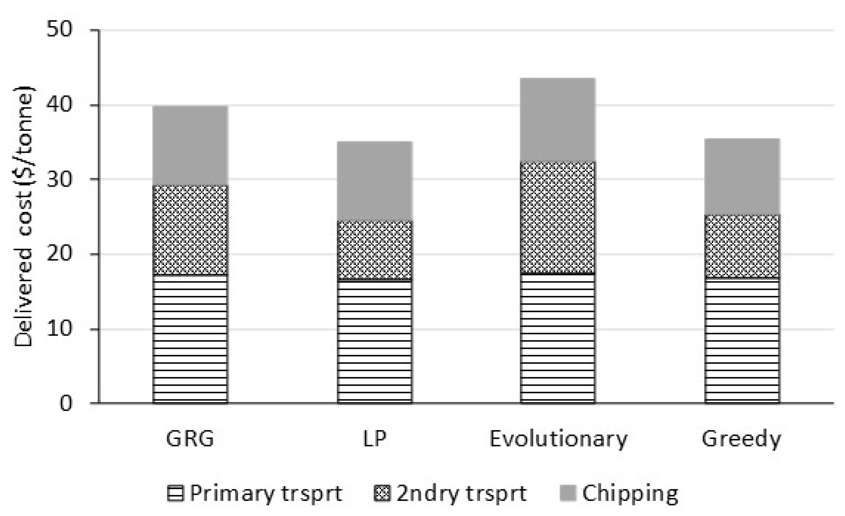
2.6.1. Stage 1: Comparison of the Performance of Four Mathematical Models

A test harness was created in MS Excel 2019 VBA to generate 100 random sets of input values within the limits defined in Table 1. The test harness solved the scheduling problem defined by each set of random input values using the three heuristic approaches (GRG, Evolutionary and Greedy) and the LP solver. The Greedy method selected the cheapest FB source each week for each customer. If there was insufficient FB to meet the customer’s weekly energy requirement, FB from the next cheapest source was used and so forth until the weekly energy requirement was fulfilled or the problem was found to be infeasible.

The test criteria used to compare the schedules from each tested method covered the useability from the planner perspective (solution time), reduction in supply chain costs (delivered cost and energy cost) and potential implementation of the schedule (remaining variables) (Table 3).

2.6.2. Stage 2: Chipper Move Cost Penalty

A cost penalty to account for transport and setup costs (AUD 3000) when moving a chipper between sites was added to the objective function for the highest performing heuristic identified in the first stage. The cost penalty was non-linear as it only applied when a chipper was not operating at a site in the previous week. The performance of the LP solver was compared with that of the heuristic algorithm with and without the chipper move cost penalty using 100 sets of random input values.

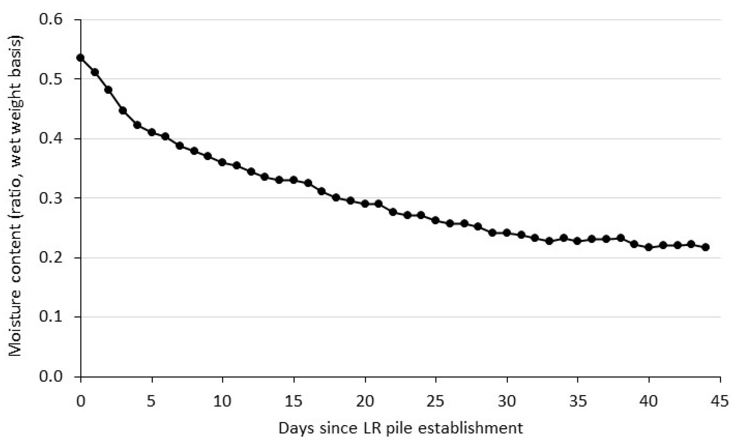
2.6.3. Stage 3: Impact of Rainfall on MC of E. nitens LR Stored at Roadside and on Its Delivery Schedule

In order to investigate the potential impacts of rainfall in the first week of the scheduled period, the test harness described previously was modified to test the three models from Stage 2 with and without simulated rainfall using 100 sets of random input values. The impact of rainfall on LR pile MC was simulated based on the response of an E. nitens LR pile to rainfall reported in [39]. This report showed that the E. nitens LR pile MC increased by approximately 5% for rainfall < 20 mm in total over several days. The initial MC for each LR pile in the DSS was increased by 5%. If this resulted in the MC exceeding the maximum starting value of 53%, the MC was set to 53%.

3. Results

3.1. Comparison of Heuristic and Linear Programming Methods

3.1.1. Stage 1: Comparison of the Performance of Four Mathematical Models

For most of the test criteria, the mean values for the LP solver and the Greedy algorithm were significantly lower than those for the other two algorithms but were not significantly different from each other (

Table 4. Mean test criteria values (non-cost) for each tested method.

Method	Time (s)	Small Load	Chippers	Max Chippers	Chipper Moves	Biomass (t)	Wtd MC%	Wtd Distance (km)	Hi-Vol Semi	Std Semi
GRG	27.8 a	32 a	70 a	9 a	11 a	8228 a	27.1 a	79 a	337 ab	431 a
LP	0.04 b	1 b	20 b	4 b	8 b	8005 a	25.1 b	44 b	331 a	431 a
Evolutionary	33.2 c	4 c	16 c	3 c	8 b	8704 b	31.1 c	98 c	350 b	431 a
Greedy	0.5 b	1 b	19 b	4 bc	7 c	7918 a	24.3 b	49 b	328 a	431 a

^a–c Means within a column sharing a superscript letter were not significantly different.

and

Table 5. Mean cost values for each tested method.

Method	Energy (AUD/GJ)	Primary Transport (AUD)	Secondary Transport (AUD)	Chipping (AUD)	Total Cost (AUD)
GRG	2.74 a	141,237 a	99,219 a	86,517 ab	326,973 a
LP	2.41 b	137,760 a	64,983 b	84,626 a	287,370 b
Evolutionary	3.01 c	142,877 a	124,899 c	90,556 b	358,333 c
Greedy	2.45 b	138,447 a	69,737 b	83,951 a	292,135 b

^a–c Means within a column sharing a superscript letter were not significantly different.

). Differences between mean values for the chipper-related test criteria for the schedules produced using the Evolutionary algorithm and those for the LP solver and Greedy algorithms were relatively small (Table 4). However, cost criteria values (particularly secondary transport costs) (Table 5) and high-volumetric capacity semi-trailer load numbers (Table 4) were higher for the Evolutionary algorithm schedules due to the significantly higher MC of the delivered biomass. The GRG algorithm schedules involved the extraction of relatively small quantities of LR from multiple sites over multiple weeks, which was reflected in the high mean values for the number of small loads and the chipper-related test criteria (Table 4).

Secondary transport cost (AUD/t) was the major cause of differences between delivered costs for the tested methods. Secondary transport costs for the Greedy algorithm and LP solver were considerably lower than those for the other two methods (Figure 3).

3.1.2. Stage 2: Chipper Move Cost Penalty

The addition of the chipper move cost penalty significantly reduced the values of the three chipper-related test criteria (

Table 6. Comparison between the LP solver and Greedy algorithm results with and without a chipper move penalty. Only test criteria with significant differences are shown.

Method	Chippers	Max Chippers	Chipper Moves
LP	20 a	4 a	8 a
Greedy	19 b	4 a	7 b
Greedy (chipper move penalty)	18 c	3 b	6 c

^a–c Means within a column sharing a superscript letter were not significantly different.

). There were no significant differences between the tested methods for the other test criteria.

3.1.3. Stage 3: Impact of Rainfall on MC of E. nitens LR Stored at Roadside and on Its Delivery Schedule

The simulated rainfall had no significant effect on the majority of the test criteria. The criteria where there was a significant difference (

Table 7. Comparison between LP solver and Greedy algorithm results with and without a chipper move penalty and with and without simulated rainfall in the first week. Only test criteria with significant differences are shown.

	Method	Chippers	Max Chippers	Chpr Moves	Wtd MC%	Wtd Dist (km)
No rain	LP	20 a	4 a	8 a	25 a	47 ab
	Greedy	19 b	4 bc	7 b	24 ab	51 ab
	Greedy (chipper move penalty)	18 c	3 d	6 cd	24 b	53 ab
Rain	LP	20 a	4 ab	8 a	29 c	46 b
	Greedy	19 b	4 bc	7 bc	27 d	53 ab
	Greedy (chipper move penalty)	18 c	3 cd	6 d	27 d	55 a

^a–d Means within a column sharing a superscript letter were not significantly different.

) mostly mirrored those in Table 6, reflecting differences between mathematical models unrelated to rainfall effects. The notable exception was the weighted biomass MC%, which was significantly greater for the results with simulated rainfall compared with those without rainfall.

4. Discussion

The study compared test solutions produced using four mathematical models (an LP solver and three heuristic algorithms (GRG non-linear, Evolutionary and Greedy)) as the basis of a “proof of concept” operational FBSC planning DSS. The comparisons were performed on the basis of solution times and objective function values and in terms of the potential for practical implementation of the solutions, which is relevant for operational level forest planning DSS but rarely evaluated.

The mean solution times and delivered costs for the LP solver and the Greedy algorithm solutions in the current study were significantly lower than those for the other two models but not significantly different from each other. Compared with the optimal value, the delivered cost for the Greedy solution was less than 2% greater whereas the delivered costs for the other two heuristic algorithms were 14–25% greater. The poor performance of the GRG and Evolutionary algorithms suggested that their solutions had converged on local minima. Their longer solution times resulted from these algorithms solving multiple problems for each solution due to the multi-start setting for the GRG algorithm and the multi-generational approach used by the Evolutionary algorithm.

The potential practical implementation of the mathematical model solutions was evaluated using four test criteria (the small load number test criterion and the three chipper-related test criteria). From the perspective of a forest planner scheduling FB deliveries, minimizing the values of each of these criteria is desirable as deliveries from sites of less than one truckload (small load number test criterion) are likely to incur a loss, chipper availability (chipper number and maximum chipper test criteria) is limited and chipper moves between sites incur a cost. The LP solver and Greedy algorithm solutions had the lowest number of small loads (1 load), but for the chipper variables, the Evolutionary algorithm solutions were equal to or better than those of the LP solver and Greedy algorithm. The mean values for the four test criteria for the GRG algorithm were significantly greater than those for the other three models which resulted in the solutions from this algorithm being unimplementable. In the second testing stage, a penalty cost for each chipper move was added to the objective function of the Greedy algorithm. This significantly reduced the mean values of all three chipper test criteria for the modified Greedy algorithm solutions without a significant increase in costs, suggesting that the modified algorithm would be the most useful to a forest planner as the basis of the operational DSS.

The majority of the savings in delivered costs for the LP solver and Greedy algorithm solutions compared with those for the other two algorithms resulted from a considerable reduction in transport costs (≥30%) associated with reduced MC values, highlighting the importance of FB drying prior to secondary transport. Drying reduced the weight of the material to be transported and reduced the quantity required to meet the customer energy requirements through increases in net calorific value. Increased net calorific value also further reduced the transport costs by reducing the proportion of LR that needed to be transported from more distant sites, as shown by the low values for both weighted MC and transport distance for the LP and Greedy algorithm solutions.

The benefit of using high-volumetric capacity trucks to transport FB dried prior to transport was highlighted with the solutions for all tested models showing that considerably fewer high-volumetric capacity truck loads than standard volume semi-trailer truck loads were required. The least number of high-volumetric capacity semi-trailer loads were required for the LP solver and Greedy algorithm solutions, reflecting their significantly lower mean weighted MC values. A reduced fleet size has a number of advantages for both the forest manager and fleet owner in terms of reduced staffing and maintenance requirements and greater social license to operate. Use of higher capacity trucks than those tested in the current study is likely to further reduce transport costs [24], though increasing truck length may reduce the harvested areas that they can access without road modifications [42].

The operational DSS in the current study could be used to identify scheduled harvest areas where delivered LR costs exceed returns. Zamora-Cristales et al. [43] suggested a similar use for their system, though they did not model the impact of roadside LR drying on delivered costs. As withdrawal of LR supply from part of the forest estate could affect energy supply commitments, this analysis needs to form part of the high-level planning processes. For areas where the DSS analysis suggested LR harvest was uneconomic, LR would be left on site, which may increase site preparation costs [32,44].

The results for the comparison of test criteria with and without simulated rainfall in the first week suggested that, overall, it made very little difference from an operational perspective, with the only significant difference of importance being the increased weighted MC% of the delivered biomass. The main reason for this was that the LR dried back to its pre-rainfall MC within several days following rain. Although the rainfall did not have a significant impact on the total quantity of delivered LR or the number of truck loads required to deliver it, there could still be an impact on the profitability of the operations if the customer paid a premium for biomass with a low MC. Higher levels of rainfall would be likely to have a bigger and more extended effect on the LR MC but were not tested.

It is an oft-repeated truism that the quality of the output from an IT system is only as good as the quality of its input data. Data quality can be defined in terms of data accuracy; timeliness, consistency, and completeness [45,46]. Audy et al. [47] found that inaccurate data concerning roadside log stocks and truck travel times were key reasons why expected savings were not being realized through the implementation of operational truck routing and scheduling DSS in Sweden and Canada. In the context of the current DSS, the estimation accuracy of the quantity and MC of forest biomass stored in roadside piles are critical to DSS solution accuracy. There is no standard method to determine the quantity of FB stored at roadside though ground-based measurements are most commonly used. Trofymow et al. [48] compared two ground-based methods used in Canada to estimate LR pile volumes with two geospatial methods (orthophotography and LiDAR) and found that the geospatial methods were able to give more accurate estimates of pile volume, but the critical error source for all methods was the estimated pile bulk density. Other approaches to estimating the mass of material in roadside LR piles include load scale-equipped forwarders [37], and models relating to pile volume and mass [49]. Reducing the estimated residue by a percentage would be a way to mitigate the risk of inaccurate pile size estimation [47]. A similar problem exists with predictions of roundwood products from inventory; however, in that case, the high value of the products and the costs of errors in inventory can justify the additional inventory accuracy. In the case of a low value product such as LR, scope for additional costs is limited. More research in this area is critical to further development of operational FBSC planning.

FB MC is generally measured by the customer upon receipt of the FB. This information can be used to check the accuracy of the modelled MC values and to make adjustments to the drying model(s) if required. Leoni et al. [50] found that the relatively new MC measurement technique of magnetic resonance was able to provide rapid MC measurements comparable in accuracy with those of the standard oven-drying technique and without the need for fuel-specific calibration required by tools based on near-infrared.

5. Conclusions

Initial testing clearly separated the four tested mathematical models into two groups: the LP solver and Greedy algorithm, which had significantly lower solution times and delivered costs than the GRG and Evolutionary algorithms. Testing the models for their suitability for practical implementation of the solutions found that the GRG algorithm solutions were unimplementable. The second testing stage found that modifying the Greedy algorithm to penalize chipper moves further reduced chipper number and moves for the solutions from this algorithm. The conclusion, therefore, was that the modified Greedy algorithm was the most suitable model to form the basis of the operational FBSC planning DSS. The use of a heuristic algorithm also simplifies the addition of further non-linear constraints compared with an LP solver.

The study identified that use of the operational DSS based on the Greedy algorithm could produce savings in delivered costs of over 10%, largely through reduced transport costs from roadside drying. However, as with most FBSC models, there was an assumption that the quantity of LR stored at roadside is accurately known and that there is little or no rain during the planning period. The study showed that up to 20 mm of rainfall in the first week of the scheduled period did not significantly effect delivered costs. Solution quality is dependent on the quality of the input data, and in the case of the proposed DSS, poor estimates of the quantity of stored FB at roadside are the key area likely to result in poor solutions. Current methods for quantity estimation can produce very inaccurate estimates. This is a critical area for further research. Until this research is conducted, a potential risk mitigation strategy is to reduce the quantity estimates by a factor.

The operational DSS developed in this paper is a first step towards a DSS that could be used by operational forest planners. User requirements were based on the authors’ experience and limited discussions with potential users. Further development of the DSS in the study would require a formal process of system development commencing with a detailed user needs analysis.

References

1. Thiffault, E.; Hannam, K.D.; Paré, D.; Titus, B.D.; Hazlett, P.W.; Maynard, D.G.; Brais, S. Effects of forest biomass harvesting on soil productivity in boreal and temperate forests—A review. Environ. Rev. 2011, 19, 278–309. [Google Scholar] [CrossRef]
2. Parikka, M. Global biomass fuel resources. Biomass Bioenergy 2004, 27, 613–620. [Google Scholar] [CrossRef]
3. Department of the Environment and Energy. Australian Energy Update 2017. Available online: https://www.energy.gov.au/sites/default/files/energy-update-report-2017.pdf (accessed on 13 December 2021).
4. De Meyer, A.; Cattrysse, D.; Rasinmäki, J.; Van Orshoven, J. Methods to optimise the design and management of biomass-for-bioenergy supply chains: A review. Renew. Sust. Energy Rev. 2014, 31, 657–670. [Google Scholar] [CrossRef] [Green Version]
5. Shabani, N.; Akhtari, S.; Sowlati, T. Value chain optimization of forest biomass for bioenergy production: A review. Renew. Sust. Energy Rev. 2013, 23, 299–311. [Google Scholar] [CrossRef]
6. Acuna, M.; Sessions, J.; Zamora, R.; Boston, K.; Brown, M.; Ghaffariyan, M.R. Methods to manage and optimize forest biomass supply chains: A review. Curr. For. Rep. 2019, 5, 124–141. [Google Scholar] [CrossRef]
7. D’Amours, S.; Epstein, R.; Weintraub, A.; Rönnqvist, M. Operations research in forestry and forest products industry. In Wiley Encyclopedia of Operations Research and Management Science; John Wiley and Sons: Hoboken, NJ, USA, 2011. [Google Scholar]
8. Malladi, K.T.; Quirion-Blais, O.; Sowlati, T. Development of a decision support tool for optimizing the short-term logistics of forest-based biomass. Appl. Energy 2018, 216, 662–677. [Google Scholar] [CrossRef]
9. Han, S.-K.; Murphy, G.E. Solving a woody biomass truck scheduling problem for a transport company in Western Oregon, USA. Biomass Bioenergy 2012, 44, 47–55. [Google Scholar] [CrossRef]
10. Pinho, T.M.; Coelho, J.P.; Oliveira, P.M.; Oliveira, B.; Marques, A.; Rasinmäki, J.; Moreira, A.P.; Veiga, G.; Boaventura-Cunha, J. Routing and schedule simulation of a biomass energy supply chain through SimPy simulation package. Appl. Comput. Inform. 2021, 17, 36–52. [Google Scholar] [CrossRef]
11. Bettinger, P.; Sessions, J.; Boston, K. A review of the status and use of validation procedures for heuristics used in forest planning. Math. Comput. For. Nat. Resour. Sci. (MCFNS) 2009, 1, 26–37. [Google Scholar]
12. Bachmatiuk, J.; Garcia-Gonzalo, J.; Borges, J.G. Analysis of the performance of different implementations of a heuristic method to optimize forest harvest scheduling. Silva Fenn. 2015, 49, 1326. [Google Scholar] [CrossRef] [Green Version]
13. Bont, L.G.; Heinimann, H.R.; Church, R.L. Concurrent optimization of harvesting and road network layouts under steep terrain. Ann. Oper. Res. 2015, 232, 41–64. [Google Scholar] [CrossRef]
14. Borges, P.; Eid, T.; Bergseng, E. Applying simulated annealing using different methods for the neighborhood search in forest planning problems. Eur. J. Oper. Res. 2014, 233, 700–710. [Google Scholar] [CrossRef]
15. Palahí, M.; Pukkala, T.; Pascual, L.; Trasobares, A. Examining alternative landscape metrics in ecological forest planning: A case for capercaillie in Catalonia. Investig. Agrar. Sist. Recur. For. 2004, 13, 527–538. [Google Scholar]
16. Boston, K.; Bettinger, P. An analysis of monte carlo integer programming, simulated annealing, and tabu search heuristics for solving spatial harvest scheduling problems. For. Sci. 1999, 45, 292–301. [Google Scholar] [CrossRef]
17. Shojaeiarani, J.; BioresourcesBajwa, D.S.; Bajwa, S.G. Properties of densified solid biofuels in relation to chemical composition, moisture content, and bulk density of the biomass. BioRes 2019, 14, 4996–5015. [Google Scholar]
18. Allen, J.; Browne, M.; Hunter, A.; Boyd, J.; Palmer, H. Logistics management and costs of biomass fuel supply. Int. J. Phys. Distrib. Logist. Manag. 1998, 28, 463–477. [Google Scholar] [CrossRef]
19. Eriksson, L.O.; Björheden, R. Optimal storing, transport and processing for a forest-fuel supplier. Eur. J. Oper. Res. 1989, 43, 26–33. [Google Scholar] [CrossRef]
20. Nurmi, J. The storage of logging residue for fuel. Biomass Bioenergy 1999, 17, 41–47. [Google Scholar] [CrossRef]
21. Lindblad, J.; Routa, J.; Ruotsalainen, J.; Kolström, M.; Isokangas, A.; Sikanen, L. Weather based moisture content modelling of harvesting residues in the stand. Silva. Fenn. 2018, 52, 7830. [Google Scholar] [CrossRef] [Green Version]
22. Petterson, M.; Nordfjell, T. Fuel quality changes during seasonal storage of compacted logging residues and young trees. Biomass Bioenergy 2007, 31, 782–792. [Google Scholar] [CrossRef]
23. Erber, G.; Kanzian, C.; Stampfer, K. Predicting moisture content in a pine logwood pile for energy purposes. Silva Fenn. 2012, 46, 555–567. [Google Scholar] [CrossRef] [Green Version]
24. Strandgard, M.; Acuna, M.; Turner, P.; Mirowski, L. Use of modelling to compare the impact of roadside drying of Pinus radiata D.Don logs and logging residues on delivered costs using high capacity trucks in Australia. Biomass Bioenergy 2021, 147, 106000. [Google Scholar] [CrossRef]
25. Strandgard, M.; Turner, P.; Mirowski, L.; Acuna, M. Potential application of overseas forest biomass supply chain experience to reduce costs in emerging Australian forest biomass supply chains—A literature review. Aust. Forestry 2019, 82, 9–17. [Google Scholar] [CrossRef]
26. Eriksson, A.; Eliasson, L.; Sikanen, L.; Hansson, P.-A.; Jirjis, R. Evaluation of delivery strategies for forest fuels applying a model for Weather-driven Analysis of Forest Fuel Systems (WAFFS). Appl. Energy 2017, 188, 420–430. [Google Scholar] [CrossRef]
27. Amrouss, A.; El Hachemi, N.; Gendreau, M.; Gendron, B. Real-time management of transportation disruptions in forestry. Comput. Oper. Res. 2017, 83, 95–105. [Google Scholar] [CrossRef]
28. Mahmoudi, M.; Sowlati, T.; Sokhansanj, S. Logistics of supplying biomass from a mountain pine beetle-infested forest to a power plant in British Columbia. Scand. J. For. Res. 2009, 24, 76–86. [Google Scholar] [CrossRef]
29. Mobini, M.; Sowlati, T.; Sokhansanj, S. Forest biomass supply logistics for a power plant using the discrete-event simulation approach. Appl. Energy 2011, 88, 1241–1250. [Google Scholar] [CrossRef]
30. Eliasson, L.; Anerud, E.; Grönlund, Ö.; von Hofsten, H. Managing moisture content during storage of logging residues at landings—Effects of coverage strategies. Renew. Energy 2020, 145, 2510–2515. [Google Scholar] [CrossRef]
31. Nilsson, B.; Nilsson, D.; Thörnqvist, T. Distributions and losses of logging residues at clear-felled areas during extraction for bioenergy: Comparing dried- and fresh-stacked method. Forests 2015, 6, 4212–4227. [Google Scholar] [CrossRef] [Green Version]
32. Strandgard, M.; Mitchell, R.; Barr, B. Final Report on SW Timber Hub Residue-Adapted Harvest Trial; South West Timber Hub: Bunbury, Australia, 2021; p. 46. Available online: https://www.swtimberhub.com.au/uploads/1/2/7/1/127157855/final_report_on_residue_adapted_trial_sw_timber_hub.pdf (accessed on 17 December 2021).
33. Acuna, M.; Anttila, P.; Sikanen, L.; Prinz, R.; Asikainen, A. Predicting and controlling moisture content to optimise forest biomass logistics. Croat. J. For. Eng. 2012, 33, 225–238. [Google Scholar]
34. Strandgard, M.; Taskhiri, M.S.; Acuna, M.; Turner, P. Impact of roadside drying on delivered costs for eucalyptus globulus logging residue and whole trees supplying a hypothetical energy plant in Western Australia using a linear-programming model. Forests 2021, 12, 455. [Google Scholar] [CrossRef]
35. Hobbs, T. Regional Industry Potential for Woody Biomass Crops in Lower Rainfall Southern Australia: FloraSearch 3c; RIRDC: Barton, Australia, 2009. [Google Scholar]
36. Senelwa, K.; Sims, R.E.H. Fuel characteristics of short rotation forest biomass. Biomass Bioenergy 1999, 17, 127–140. [Google Scholar] [CrossRef]
37. Strandgard, M.; Mitchell, R. Comparison of cost, productivity and residue yield of cut-to-length and fuel-adapted harvesting in a Pinus radiata D.Don final harvest in Western Australia. N. Z. J. For. Sci. 2019, 49, 209451403. [Google Scholar] [CrossRef] [Green Version]
38. Zamora-Cristales, R.; Boston, K.; Sessions, J.; Murphy, G. Stochastic simulation and optimization of mobile chipping economics in processing and transport of forest biomass from residues. Silva Fenn. 2013, 47, 937. [Google Scholar] [CrossRef] [Green Version]
39. Strandgard, M.; Mitchell, R.; Acuna, M.; Ghaffariyan, M.; Brown, M. Control and Manage the Moisture Content of Logs and Biomass to Maximise Benefits along the Wood Supply Chain; Forest and Wood Products Australia (FWPA): Melbourne, Australia, 2020; Available online: https://www.fwpa.com.au/images/processing/2020/Final_Report_PNC400-1516.pdf (accessed on 17 December 2021).
40. Elbersen, W.; Lammens, T.M.; Alakangas, E.A.; Annevelink, B.; Harmsen, P.; Elbersen, B. Chapter 3—Lignocellulosic biomass quality: Matching characteristics with biomass conversion requirements. In Modeling and Optimization of Biomass Supply Chains; Panoutsou, C., Ed.; Academic Press: Cambridge, MA, USA, 2017; pp. 55–78. [Google Scholar]
41. Vaezi, M.; Kabir, M.R.; Kumar, A. Monitoring moisture and inorganic content of forest harvesting residues for energy production purposes: A case study. Can. Biosyst. Eng. 2019, 61, 8–12. [Google Scholar] [CrossRef]
42. Zamora-Cristales, R.; Sessions, J.; Boston, K.; Murphy, G. Economic optimization of forest biomass processing and transport in the Pacific Northwest USA. For. Sci. 2015, 61, 220–234. [Google Scholar] [CrossRef]
43. Zamora-Cristales, R.; Boston, K.; Long, J.; Sessions, J. Economic estimation of the available biomass following logging operations in Western Oregon and Washington. For. Prod. J. 2018, 68, 191–198. [Google Scholar] [CrossRef] [Green Version]
44. Strandgard, M.; Béland, M. Economics of forest biomass for bioenergy: Potential site preparation savings from coarse woody harvesting residue removal in a short-rotation Eucalyptus globulus (Labill.) plantation. Silva Balc. 2021, 22, 45–55. [Google Scholar] [CrossRef]
45. Batini, C.; Cappiello, C.; Francalanci, C.; Maurino, A. Methodologies for data quality assessment and improvement. ACM Comput. Surv. 2009, 41, 16. [Google Scholar] [CrossRef] [Green Version]
46. Hazen, B.T.; Boone, C.A.; Ezell, J.D.; Jones-Farmer, L.A. Data quality for data science, predictive analytics, and big data in supply chain management: An introduction to the problem and suggestions for research and applications. Int. J. Prod. Econ. 2014, 154, 72–80. [Google Scholar] [CrossRef]
47. Audy, J.-F.; Lidén, B.; Favreau, J. Issues and solutions for implementing operational decision support system—An application in truck routing and scheduling system. In Proceedings of the 4th Forest Engineering Conference: Innovation in Forest Engineering—Adapting to Structural Change, White River, South Africa, 5–7 April 2011. [Google Scholar]
48. Trofymow, J.A.; Coops, N.C.; Hayhurst, D. Comparison of remote sensing and ground-based methods for determining residue burn pile wood volumes and biomass. Can. J. For. Res. 2013, 44, 182–194. [Google Scholar] [CrossRef]
49. Fernandez-Lacruz, R.; Bergström, D. Windrowing and fuel-chip quality of residual forest biomasses in northern Sweden. Int. J. For. Eng. 2017, 28, 186–197. [Google Scholar] [CrossRef]
50. Leoni, E.; Mancini, M.; Aminti, G.; Picchi, G. Wood fuel procurement to bioenergy facilities: Analysis of moisture content variability and optimal sampling strategy. Processes 2021, 9, 359. [Google Scholar] [CrossRef]
Figure 1. Biomass supply chain showing the major activities. Activities in the dashed box are included in the current DSS.
Forests 13 00138 g001
Figure 2. E. nitens (H.Deane & Maiden) Maiden LR drying model based on the model published in [39] with the rain response removed.
Forests 13 00138 g002
Figure 3. Mean delivered cost (AUD/tonne) for each tested method divided into primary and secondary transport and chipping costs.
Forests 13 00138 g003