Comparison of Data Grouping Strategies on Prediction Accuracy of Tree-Stem Taper for Six Common Species in the Southeastern US

Abstract

Clustering data into similar characteristic groups is a commonly-used strategy in model development. However, the impact of data grouping strategies on modeling stem taper has not been well quantified. The objective of this study was to compare the prediction accuracy of different data grouping strategies. Specifically, a population-level model was compared to the models fitted with grouped data based on taxonomic rank, tree form and size. A total of 3678 trees were used in the analyses, which included six common species in upland hardwood forests of the southeastern U.S. Results showed that overall predictions are more accurate when building stem taper models at the species, species group or division level rather than at the population level. The prediction accuracy was not considerably improved between species-specific functions and models fitted with species-related groups for the four hardwood species examined. Grouping data by taxonomic rank provided more reliable predictions than height-to-diameter ratio (H–D ratio) or diameter at breast height (DBH). The form/size-related grouping methods (i.e., data grouped by H–D ratio or DBH) generally did not improve the prediction precision compared to a population-level model. In this study, the effect of sample size in model fitting showed a minimal impact on prediction accuracy. The methodology presented in this study provides a modeling strategy for mixed-species data, which will be of practical importance when data grouping is needed for developing stem taper models.

1. Introduction

Tree-stem taper, defined as the change in tree diameter with increasing tree height from ground level to total tree height, is a quantitative description of stem profile [1]. For a given population, stem taper functions are typically built by species, also known as species-specific models, e.g., [2,3,4]. Since every species in a plant community may respond differently to environmental and management changes and conditions, developing stem taper models at the species level has been generally assumed to better capture variable tree forms compared to a single population or community-level model (i.e., a single taper model for the entire population) [5,6]. However, building species-specific models usually requires relatively large samples due to complex model forms and large numbers of parameters [7]. When the target population includes a variety of species (e.g., mixed-hardwood forests), especially if many of them are recorded infrequently or are sparse in the population, fitting stem taper models by species can be difficult under time and cost constraints. Rather than grouping data at the species level, an alternative approach is to re-aggregate individuals into a smaller number of groups based on similar tree characteristics (e.g., taxonomic rank, tree form, size). This approach is cost-efficient when quantifying stem profile with limited data for diverse species, e.g., [8].

In model evaluation, prediction accuracy is an important criterion and is commonly assessed using an independent validation dataset. It was found that parametric stem taper models produced reliable predictions for loblolly pine when the size distribution of the predicted populations deviated from the observations used in model development (i.e., high robustness) [9]. Although the data grouping approach has been implemented in forest and natural resources practice, to our knowledge, the accuracy of stem taper models fit by different data grouping approaches and calibration sample sizes has not been extensively investigated. Stem taper modeling has primarily focused on single stemmed, excurrent crown form trees (e.g., coniferous species), e.g., [10,11,12,13]. Predicting stem taper for decurrent trees (e.g., deciduous hardwoods) is generally more challenging than excurrent trees due to a more complicated geometric shape of the main stem [1,8]. Although stem taper equations for upland hardwoods in the southeastern US were built in the past, e.g., [4], the predictability of models under various data grouping strategies has not been extensively examined.

Therefore, the objectives of this study were (1) to compare the prediction accuracy among different data grouping strategies, and (2) to examine the effect of sample size on the prediction accuracy of stem taper with different data grouping strategies. To achieve the first objective, stem taper models fit at the population level (i.e., one taper model for the entire dataset) were compared with those grouped based on taxonomic rank, tree form and size. Specifically, trees were grouped by species (species-specific), species group, division (phylum) group (i.e., softwoods vs. hardwoods), height–DBH ratios (H–D ratios) or DBH, respectively. For the second objective, trees were split randomly between a fitting and validation set at 10/90, 20/80, 30/70, 40/60, 50/50, 60/40, 70/30, 80/20 and 90/10 splits. For example, with a 20/80 split, 20% of the trees were randomly selected as fitting data, and the remaining 80% were used for validation. Six common species in the upland hardwood forests in the southeastern US were selected, including shortleaf pine (Pinus echinata), Virginia pine (Pinus virginiana), yellow poplar (Liriodendron tulipifera), hickory spp. (Carya spp.), white oak (Quercus alba) and southern red oak (Quercus falcata). These species are economically and ecologically important in the region [14]. The results of this study will provide insights on selecting appropriate data grouping strategies when developing tree-taper models with inadequate per-species data.

2. Materials and Methodology

2.1. Data

The stem taper data used in this study were collected from the LegacyTree database (http://www.legacytreedata.org, last accessed on 18 October 2021). The LegacyTree database is a large compilation of North American trees sampled in the past century [15]. Felled trees with measured diameter outside bark (d, cm), diameter at breast height (DBH, cm) and total tree height (Ht, m) were used in analysis. The average taper trends and distributions of height to DBH ratios (H–D ratios) are shown in Figure 1. The sample trees were collected from 13 states in the southeastern US, including Alabama, Arkansas, Florida, Georgia, Kentucky, Louisiana, Mississippi, North Carolina, Oklahoma, South Carolina, Tennessee, Texas and Virginia. After trees with DBH < 7.6 cm (3 in) and total tree height < 4.6 m (15 ft) were excluded [16], a total number of 3678 trees were obtained. To reduce the sources of uncertainty in data collection, only a single dataset collected by Clark et al. [4] was used in this work. A summary of tree characteristics for each species is given in

Table 1. Summary statistics of tree characteristics for the six species evaluated. N_tree is the total number of sample trees, and N_obs/tree is number of observations (taper points) per tree. DBH is diameter at breast height in cm, and Ht is total tree height in m. For N_obs/tree, DBH and Ht, the average is given followed by standard deviation in parentheses.

Species	Ntree	Nobs/tree	DBH (cm)	Ht (m)
shortleaf pine (Pinus echinata Mill.)	1347	24 (4)	35.2 (10.5)	21.8 (3.8)
Virginia pine (Pinus virginiana Mill.)	345	22 (3)	29.2 (7.5)	20.6 (3.4)
white oak (Quercus alba L.)	717	25 (4)	36.9 (10.0)	23.7 (3.5)
southern red oak (Quercus falcata Michx.)	292	24 (3)	37.1 (8.6)	22.4 (2.9)
yellow poplar (Liriodendron tulipifera L.)	399	28 (4)	40.0 (11.7)	28.5 (4.8)
hickory spp. (Carya spp.)	578	25 (4)	35.4 (10.2)	24.0 (3.9)

.

2.2. Taper Model

Models proposed by Kozak [12] and Max and Burkhart [11] were applied to predict stem tapers. Due to their flexibility, both models have been widely used to describe the tree profiles for a variety of species in different regions [10].

2.2.1. Variable-Exponent Model

The nine-parameter variable-exponent model proposed by Kozak [12] can be written as:

$$\mathrm{d} ={ \mathrm{a}}_0{\mathrm{DBH}}^{{\mathrm{a}}_1}{\mathrm{Ht}}^{{\mathrm{a}}_2}{ \mathrm{K}}^{\mathrm{z}}$$

(1)

where

$$\mathrm{K}=\left[1-{\left(\frac{\mathrm{h}}{\mathrm{Ht}}\right)}^{\frac{1}{3}}\right]/\left[1-{\left(\frac{1.3}{\mathrm{Ht}}\right)}^{\frac{1}{3}}\right]$$

(2)

$$\mathrm{Z}={\mathrm{a}}_3{\left(\frac{\mathrm{h}}{\mathrm{Ht}}\right)}^4+{\mathrm{a}}_4\left[\frac{1}{{\mathrm{e}}^{\left(\frac{\mathrm{DBH}}{\mathrm{Ht}}\right)}}\right]+{\mathrm{a}}_5{\mathrm{K}}^{0.1}+{\mathrm{a}}_6\left(\frac{1}{\mathrm{DBH}}\right)+{\mathrm{a}}_7{\mathrm{Ht}}^{\left[1-{\left(\frac{\mathrm{h}}{\mathrm{Ht}}\right)}^{\frac{1}{3}}\right]}+{\mathrm{a}}_8\mathrm{K}$$

(3)

and a₀–a₈ are model coefficients. In some cases, this model form can produce negative value of Z when K = 0 (h = Ht), leading to an undefined value of d. Thus, when h = Ht, the restriction of d = 0 was imposed to Equation (1).

2.2.2. Segmented Polynomial Regression Model

Max and Burkhart [11] proposed using the squared ratio d²/DBH² as the dependent variable, but Yang and Burkhart [9] found that the model with the first order ratio d/DBH provided more accurate predictions. To be comparable with the Kozak [12] model, the model with the first order ratio was used in this study, which is

$$\mathrm{d}/\mathrm{DBH} ={ \mathrm{a}}_0\left(\mathrm{x}-1\right)+{ \mathrm{a}}_1\left({\mathrm{x}}^2-1\right)+{ \mathrm{a}}_2{\left({\mathrm{b}}_1-\mathrm{x}\right)}^2{\mathrm{I}}_1+{ \mathrm{a}}_3{\left({\mathrm{b}}_2-\mathrm{x}\right)}^2{\mathrm{I}}_2$$

(4)

where x is h/Ht, a₀−a₃ are model coefficients,

$$\begin{array}{ll}{\mathrm{I}}_1& = 1, \mathrm{if} {\mathrm{b}}_1\ge \mathrm{x}\\ & = 0, \mathrm{if} {\mathrm{b}}_1<\mathrm{x}\end{array}$$

and

$$\begin{array}{ll}{\mathrm{I}}_2& = 1, \mathrm{if} {\mathrm{b}}_2\ge \mathrm{x}\\ & = 0, \mathrm{if} {\mathrm{b}}_2<\mathrm{x}\end{array}$$

In Max and Burkhart [11] model, coefficients b₁ and b₂ are used to join three segments of tree stems to form a single model, which were estimated as 0.69 and 0.11, respectively, using all tree-stem taper data in this study. The fixed estimates of b₁ and b₂ were applied to all cases listed in Section 2.3.

2.3. Model Fitting and Evaluation

The step-by-step procedure of tree selection for model fitting and validation is given as:

• A random sample of 100 trees was selected from the original dataset for a given species.
• (a)

  Population-level case (fitting a single stem taper model for all data):

  For a given species, 100 sample trees selected in step 1 were randomly split into fitting and validation datasets based on step 3. Then, the randomly-split trees were merged into a fitting and validation dataset, respectively. In this case, fitting and validation datasets included all species, and each species contributed equal number of trees.

  (b)

  Data grouping cases (fitting stem taper with grouped data):

  Trees drawn from step 1 were grouped based on taxonomic rank, tree form and size, which were detailed in Section 2.3.1 and Section 2.3.2.

• Fitting and validation data were created with 10/90, 20/80, 30/70, 40/60, 50/50, 60/40, 70/30, 80/20 and 90/10 splits. Trees used in fitting and validation were randomly selected. Model parameters were estimated with the Levenberg–Marquardt (LM) non-linear least squares algorithm that is implemented in the nlsLM function in R [17]. The LM algorithm is a compromise between the gradient-descent and Gauss–Newton approaches, which leads to more stable parameter estimates [18]. The initial values for parameter estimation were obtained from Yang and Burkhart [9]. The model evaluation statistics are given in Section 2.3.3.
• Steps 1–3 were repeated 500 times.

To provide comparable results, the total number of sampling trees summed from all groups was 600 (i.e., 600 = 100 trees/species × 6 species), which was consistent for all cases (i.e., population level and data grouping cases). When a tree was selected, all stem taper measurements within the tree were included, so that the correlation structure of repeated measurements was retained (i.e., cluster sampling).

2.3.1. Grouping Data Based on Taxonomic Rank

Three ranks in the taxonomic hierarchy: species-specific, species group and divisions, were used in data grouping. The methods were defined as:

• Trees grouped by species (fitting stem taper at species level):
  All trees selected in step 1 were used in model fitting and evaluation where fitting and validation datasets included only a single species. For a given species, 100 sample trees selected in step 1 were randomly split into fitting and validation datasets based on step 3.
• Trees grouped by species group:
  Six species were divided into three species groups: pine (shortleaf pine and Virginia pine), oak (white oak and southern red oak) and other hardwoods (yellow poplar and hickory spp.). Species in the pine or oak groups belong to the same genus. Although yellow popular and hickory spp. were in different genera, the classifying strategy is commonly implemented in practice when species data are not available [4]. For a given group, the fitting/validation datasets were composed of equal proportion of sample trees from each species. For example, under the 90/10 split, each species in a group contributed 90 trees for fitting and 10 trees for validation.
• Trees grouped by division group (gymnosperm vs. angiosperm):
  Six species were divided into softwood and hardwood groups. The softwood group included short-leaf pine and Virginia pine, whereas the other group contained white oak, southern red oak, yellow poplar and hickory spp. For a given group, the fitting/validation datasets were composed of equal proportion of sample trees from each species. Each species in a group has 100 trees randomly selected for fitting and validation.

Notably, data splitting was species-independent. When species were mixed, the fit- ting/validation data included the same number of trees from each species. For example, when species A and B are mixed, each species provides 100 trees. Given the 90/10 split, 90 trees were selected for fitting from the 100 trees of each species and the validation data included the remaining 10 trees (i.e., 10 = 100 − 90) from species A and B, respectively.

2.3.2. Grouping Data Based on Tree Form and Size

In this scenario, the sample trees of the six species selected in step 1 were merged into a dataset (a total of 600 trees, 600 = 100 × 6), and then regrouped into k number of equal-sized groups by H–D ratios or DBH. A taper function was applied to each of k groups, where k is equal to 6, 3 and 2 (i.e., 6, 3 and 2 groups). Specifically,

• Six HD ratio or DBH groups: Trees were divided into six groups based on H–D ratios or DBH. Each group included 100 trees (i.e., 100 trees/group = 600 trees/6 groups).
• Three H–D ratio or DBH groups: Trees were divided into the smallest, middle and largest one-thirds based on H–D ratios or DBH to generate three H–D ratio or DBH groups. Each group included 200 trees (i.e., 200 trees/group = 600 trees/3 groups).
• Two H–D ratio or DBH groups: Trees were divided into the smallest and largest 50% based on H–D ratios or DBH to generate two H–D ratio or DBH groups. Each group included 300 trees (i.e., 300 trees/group = 600 trees/2 groups).

2.3.3. Statistics for Model Evaluation

To evaluate the accuracy of stem diameter prediction, the percent mean bias (MB) and percent root mean square error (RMSE) for a given repetition were calculated as

$$\mathrm{MB}=\frac{{\displaystyle \sum }{ \mathrm{e}}_{\mathrm{d}}/\mathrm{d}}{\mathrm{N}}\ast 100\%$$

(5)

$$\mathrm{RMSE}={\left[\frac{{\displaystyle \sum }{\left({\mathrm{e}}_{\mathrm{d}}/\mathrm{d}\right)}^2}{\mathrm{N}}\right]}^{\frac{1}{2}}\ast 100{\%}^{ }$$

(6)

where N is the total number of observations in a sample, and the residuals for stem taper points (${\mathrm{e}}_{\mathrm{d}}$, cm) were calculated as

$${\mathrm{e}}_{\mathrm{d}}= \mathrm{d}- \hat{\mathrm{d}}$$

(7)

where d and $\hat{\mathrm{d}}$ are the observed and predicted diameters in cm, respectively. For a given group, the estimates and 95% confidence intervals of MB and RMSE were computed by the median, 2.5% and 97.5% quantiles of 500 repetitions. Then, the overall estimates and 95% confidence intervals of MB and RMSE were calculated by averaging all groups for a given case.

3. Results

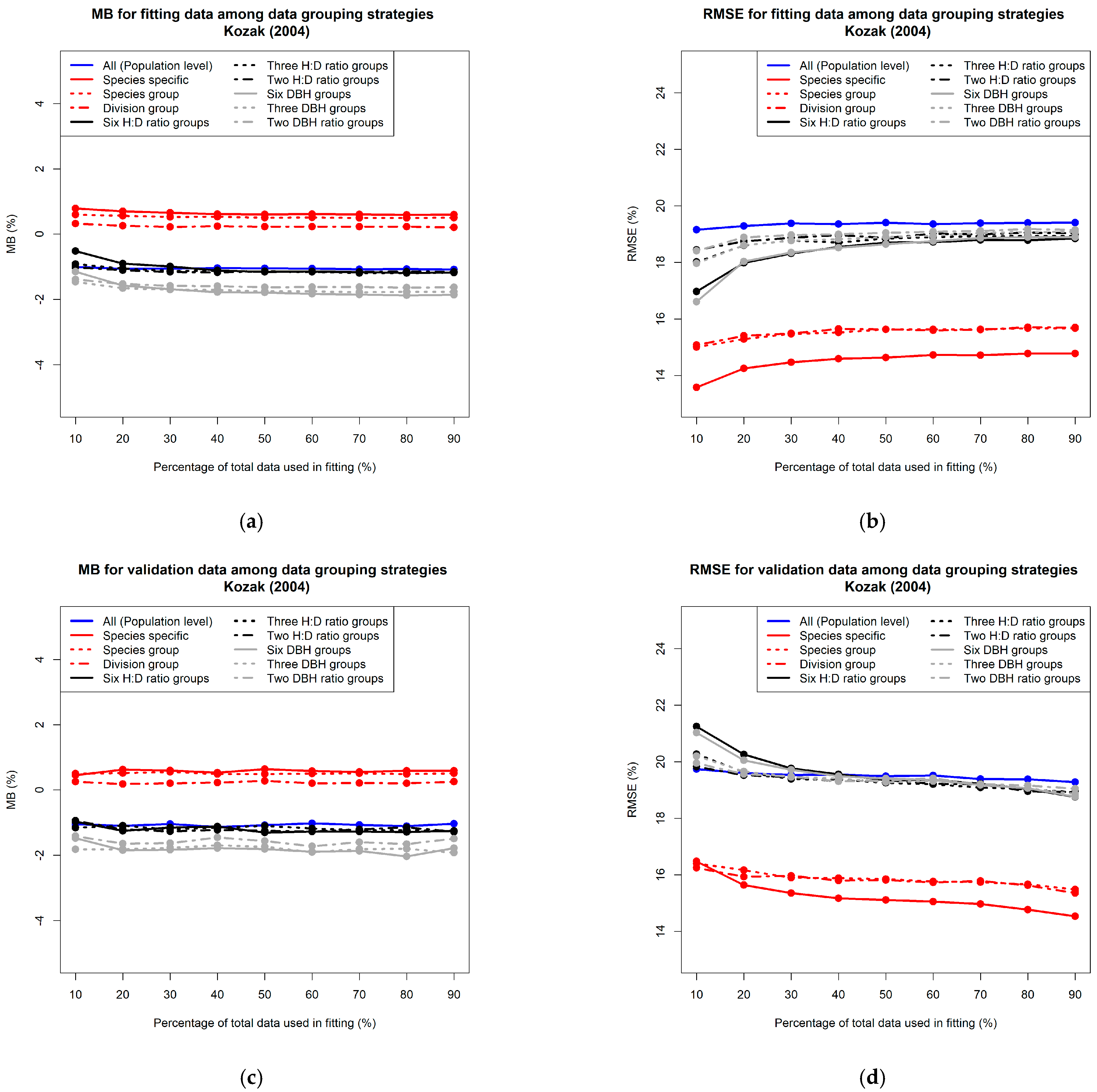
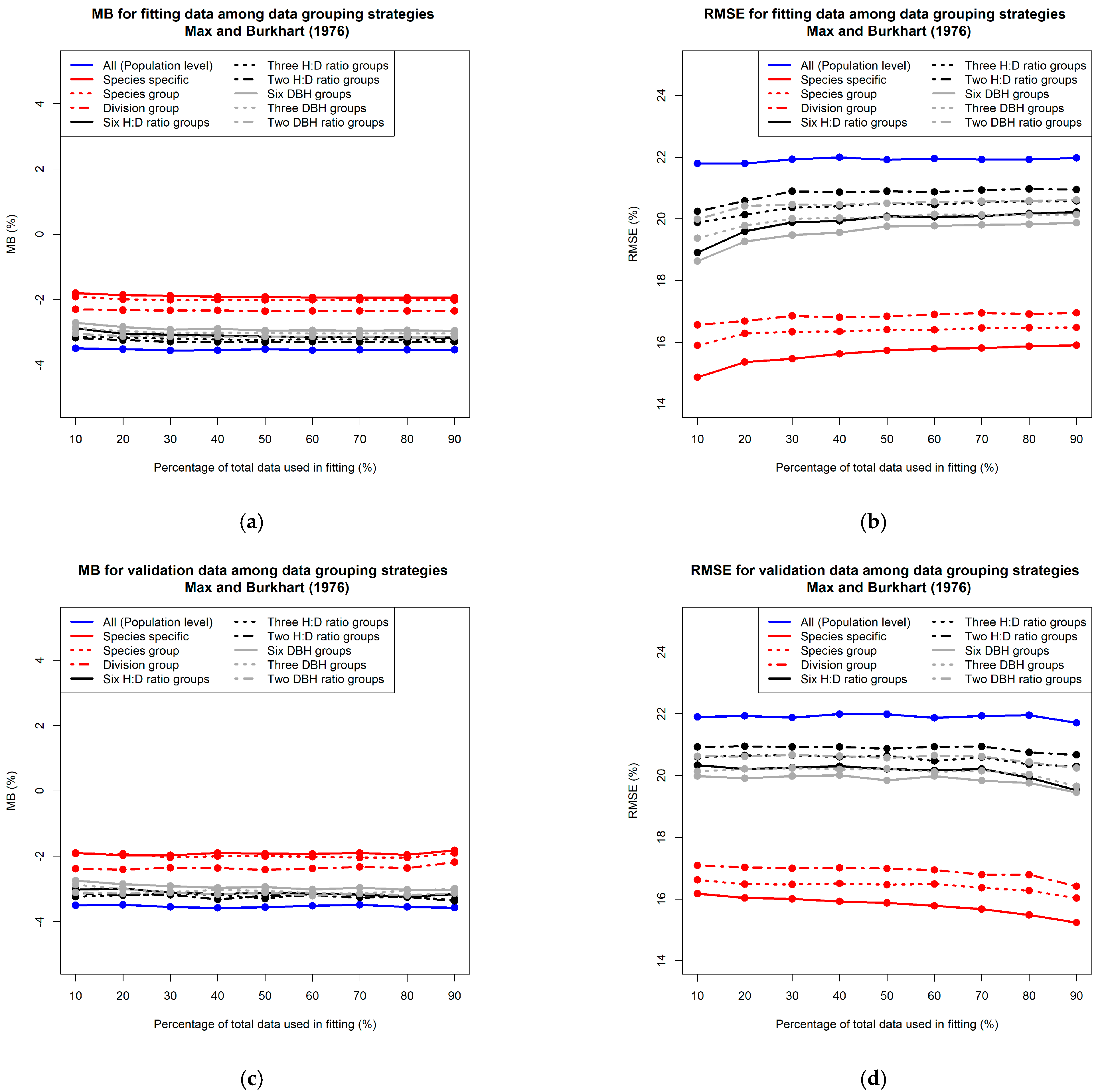
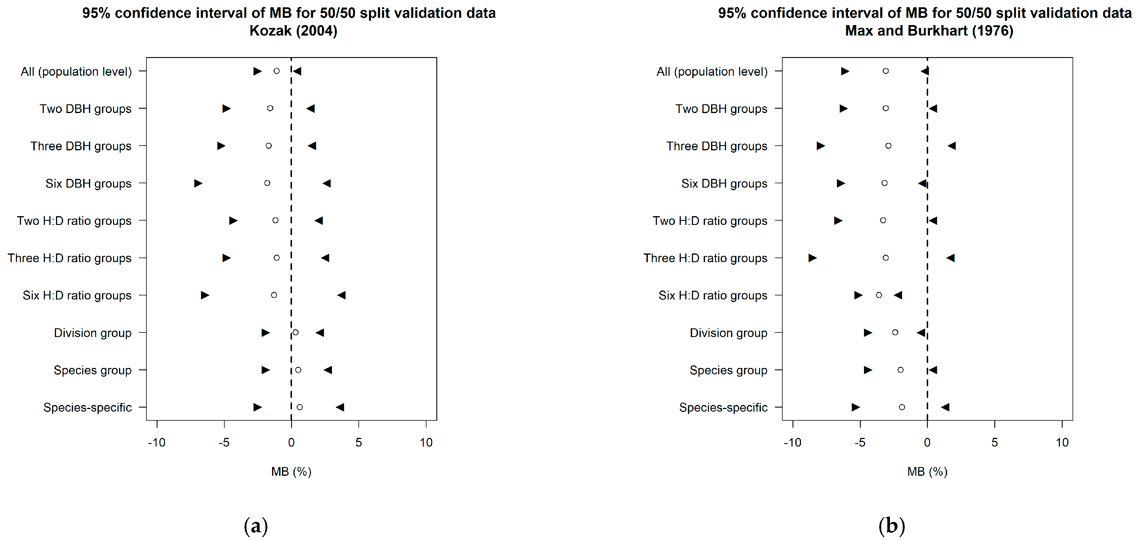
3.1. Comparison of Prediction Accuracy among Different Data Grouping Strategies

3.1.1. Grouping Data Based on Taxonomic Rank

Overall, species-specific models provided more accurate predictions of stem taper than those fit at population level (see percent MB and RMSE in Figure 2 and Figure 3). When data were grouped by taxonomic rank, the three methods yielded similar mean bias regardless of fitting/validation data or model form. Generally, the overall prediction of stem taper was more precise when the data were divided by the lower rank of taxonomic hierarchy (i.e., species level) than the higher tank, but the improvements were minimal. As shown in Figure 2 and Figure 3, the models fitted by species provided smaller RMSE than the models fitted by the other species-related groups (i.e., data grouped by species group or division). However, the differences were only about 2% for fitting, and less than 2% in validation for both the Kozak (2004) and Max and Burkhart (1976) models.

We further examined model validation by species. As

Table 2. Summary of percent mean bias (MB) and percent root mean square error (RMSE) for validation among six species by Kozak (2004) and Max and Burkhart (1976) models. Fitting/validation datasets were split as 10/90, 50/50 and 90/10 (%), respectively.

			Mean Bias (%)			RMSE (%)
Model	Species	Grouping	10/90	50/50	90/10	10/90	50/50	90/10
Kozak (2004)	shortleaf pine (Pinus echinata Mill.)	Species-specific	−1.3	−0.8	−0.8	14.3	12.7	11.8
		Species group	3.2	2.8	2.9	13.4	12.5	11.8
		Division group	3.0	2.9	2.8	13.4	12.5	11.7
		Population level	15.0	15.1	15.0	23.5	23.4	23.3
	Virginia pine (Pinus virginiana Mill.)	Species-specific	−1.0	−0.6	−0.9	14.3	13.1	12.7
		Species group	−4.9	−5.2	−5.1	17.6	17.3	17.0
		Division group	−5.3	−5.2	−5.0	17.8	17.5	16.7
		Population level	5.7	5.6	5.9	15.8	15.3	15.1
	yellow poplar (Liriodendron tulipifera L.)	Species-specific	0.9	1.0	0.9	15.2	13.9	13.2
		Species group	1.6	1.6	1.6	15.5	14.7	13.9
		Division group	2.1	2.1	2.3	16.1	15.6	14.9
		Population level	−2.9	−3.1	−2.7	15.7	15.3	14.0
	white oak (Quercus alba L.)	Species-specific	1.6	1.7	1.8	17.7	16.3	15.7
		Species group	1.5	1.9	2.0	17.3	16.6	16.3
		Division group	1.9	1.9	1.9	16.8	16.2	15.8
		Population level	−6.5	−6.5	−6.3	19.7	19.1	18.5
	southern red oak (Quercus falcata Michx.)	Species-specific	1.5	1.7	1.6	18.2	17.0	16.7
		Species group	1.3	1.3	1.4	17.0	16.7	16.6
		Division group	1.2	1.0	1.0	16.7	16.4	15.8
		Population level	−8.7	−8.5	−8.5	21.4	21.1	20.6
	hickory spp. (Carya spp.)	Species-specific	1.0	0.9	1.0	19.2	17.5	17.2
		Species group	0.3	0.0	0.2	17.2	16.7	16.2
		Division group	1.0	0.9	1.0	17.5	17.2	16.6
		Population level	−7.3	−7.3	−7.2	21.0	20.7	20.2
Max and Burkhart (1976)	shortleaf pine (Pinus echinata Mill.)	Species-specific	−2.9	−2.7	−2.5	15.6	15.2	14.3
		Species group	0.7	0.8	1.0	13.9	13.7	13.1
		Division group	0.8	0.7	1.2	14.0	13.6	12.7
		Population level	13.4	13.3	13.3	20.1	19.9	19.6
	Virginia pine (Pinus virginiana Mill.)	Species-specific	−3.6	−3.5	−3.6	18.1	18.2	17.7
		Species group	−7.7	−7.7	−7.1	21.8	21.7	21.0
		Division group	−7.6	−7.7	−7.2	21.9	21.7	20.7
		Population level	5.7	5.6	5.7	15.2	15.1	14.8
	yellow poplar (Liriodendron tulipifera L.)	Species-specific	−2.1	−2.1	−1.9	16.0	15.9	14.9
		Species group	−0.4	−0.6	−0.4	14.9	14.7	13.7
		Division group	0.4	0.5	0.7	14.6	14.4	13.5
		Population level	−7.4	−7.5	−7.6	19.9	19.8	19.2
	white oak (Quercus alba L.)	Species-specific	−0.9	−1.0	−0.9	15.4	14.9	14.3
		Species group	−0.2	−0.3	−0.1	15.1	14.7	14.0
		Division group	−1.7	−1.5	−1.4	15.8	15.3	14.6
		Population level	−9.3	−9.3	−8.9	23.6	23.6	22.5
	southern red oak (Quercus falcata Michx.)	Species-specific	−0.9	−1.1	−1.0	15.4	15.0	14.6
		Species group	−1.7	−1.7	−1.8	15.4	15.2	14.5
		Division group	−3.2	−3.2	−3.1	16.4	16.3	15.6
		Population level	−11.1	−11.2	−11.1	25.5	25.6	25.1
	hickory spp. (Carya spp.)	Species-specific	−1.1	−1.2	−1.0	16.5	16.2	15.7
		Species group	−2.8	−3.0	−3.0	17.7	17.7	17.1
		Division group	−2.1	−2.1	−2.0	16.8	16.7	15.8
		Population level	−9.7	−9.9	−9.6	24.5	24.8	23.8

shows, all six species showed improvements in prediction accuracy when changing from a population-level model to the models fitted by species-related groups except for Virginia pine with the Max and Burkhart [11] model. With the Kozak [12] model, the largest reduction in MB and RMSE between species-specific and population-level models was found for shortleaf pine, ranging from approximately 15% for MB and 10% for RMSE, followed by oaks and hickory. Similar results were found using the Max and Burkhart [11] model with larger RMSE improvements being realized for the oak and hickory species. The differences in accuracy between the population-level and species-grouping models for yellow poplar were relatively small compared to other species using the Kozak [12] model. Notably, for Virginia pine, the model fitted with species group or division group yielded lower precision than the species-level model, which may be because it was grouped with shortleaf pine. Furthermore, when building models at the species level, excurrent trees (shortleaf pine, Virginia pine and yellow poplar) showed a lower RMSE than decurrent trees (white oak, southern red oak and hickory) (Table 2), which implied that excurrent trees had a lower variation in stem profile among individuals. Notably, grouping data by three different taxonomic ranks for the four hardwood species did not show noticeable differences in prediction accuracy (see MB and RMSE in Table 2). Precision was not greatly decreased using a species-specific model compared with higher-level groupings for both model forms. In other words, building stem taper models with species-specific (a lower rank in taxonomic hierarchy) did not greatly improve the prediction accuracy. For example, a similar range of RMSE was produced (15.7–17.7% and 16.3–17.3%, respectively, in Table 2) when fitting white oak alone or white oak in the oak group with the Kozak [12] model.

3.1.2. Grouping Data Based on Tree Form and Size

When H–D ratio or DBH was used in data grouping, the overall absolute mean bias was similar to the species-related grouping models. Based on 95% confidence intervals shown in Figure 4, the [12] model yielded fewer biased predictions than the [11] model. For RMSE, the average differences increased to 4–5% (Figure 2 and Figure 3). In some cases, using the form/size-grouping methods produced less precise predictions than the population-level model (See Figure 2d). Unlike using taxonomic rank in data grouping, the results showed that increasing the number of H–D ratio or DBH groups in model fitting did not appreciably improve the prediction accuracy. As Figure 2 and Figure 3 illustrate, MB and RMSE were similar among the different number of H–D ratio/DBH groups. Although H–D ratio has been shown to be related to crown/tree form, and tree taper usually varies by tree DBH, e.g., [8,9,19,20], we found that the uncertainty of prediction was not considerably reduced when grouping data based on H–D ratio or DBH.

3.2. Effect of Sample Size on Prediction Accuracy

Generally, the effect of sample size used for model fitting was small except for the form/size-grouping methods with the Kozak (2004) model. Taper models were robust across all fitting/validation ratios evaluated. Larger sample sizes minimally affected MB for both the fitting and validation data regardless of grouping strategies (Figure 2 and Figure 3). Larger fitting sample sizes resulted in slightly larger RMSE values; however, the validation RMSE values noticeably improved with larger fitting sample sizes, especially when changing from 10% to 20% of the total data with the Kozak [12] model used (Figure 2 and Figure 3). The largest improvement in fit statistics for RMSE occurred with the six H–D ratio grouping strategy with an approximate 3% improvement from the smallest fitting size to the largest.

4. Discussion

In forestry, grouping data by species to build species-specific taper models has long been assumed as the most accurate and precise strategy among other data clustering methods. Grouping data by other criterion (e.g., higher taxonomic rank) was viewed as a compromise when sufficient species-level observations were lacking. This resulted in most of the past efforts being confined to developing statistical methods for species-level models with a limited sample size. However, our results showed that grouping data by species did not greatly improve the prediction accuracy of stem taper compared to clustering data by species group or division. Grouping data by the higher rank of taxonomic hierarchy may still provide a certain level of accuracy in prediction. Notably, in this study, Virginia pine was grouped with shortleaf pine because they are the only two coniferous pine species. However, both species could have variable size and stem shape, which results in poor prediction accuracy when both species were grouped (see Figure 1 and Table 1). We found that species-specific models could be less precise than those fit to higher levels of grouping for a given species as an individual species may contain considerable variation in stem taper depending on growing conditions.

Clustering data into a small number of similar, simplified groups has been examined and implemented in forestry and ecology. However, many of the past studies were primarily focused on grouping data from ecological perspectives (e.g., aggregating data into functional groups) in species-abundant forest ecosystems (e.g., tropical rain forests), e.g., [19,21,22]. The results showed that using only H–D ratio or DBH as a grouping criterion was not adequate to accurately classify data so that the individuals within groups have more similar taper than those between groups (i.e., the variation within groups is smaller than that between groups.). Using multiple criteria (e.g., a combination of species and tree size) in data grouping may improve the overall prediction accuracy, but adding additional criteria usually requires a larger sample size in model development. Thus, in this study, the data were classified by only a single criterion at a time, so that the results can be better implemented in forestry practice.

When handling mixed-species data, the primary goal usually lies in finding a proper modeling strategy for minimizing the uncertainty for all species, not just for a single species. Grouping data by species group or division was found to not cause a large reduction in precision and accuracy in prediction. In other words, the influence of grouping by upper levels of taxonomic rank was minimal and dependent on the population of interest. Various statistical methods have been widely studied for modeling stem taper in the forestry literature [10]; however, to our knowledge, the impact of grouping strategies on predicting stem taper has not been extensively examined. The findings of this work can be used to provide insights in building stem taper models for multi-species datasets. In addition to the six species examined, the methodology can be applied to other types of forests when data clustering is needed.

Other than aggregating data, an alternative approach for dealing with multi-species data is to construct a population-level, mixed-effect model, and localize the equation with the upper stem diameter of the target trees, e.g., [23]. However, measuring upper stem diameters requires additional time and effort in the field, which may not be a feasible option in many cases. Lam et al. [24] proposed adding the taxonomic hierarchy of genus and species as random effects in developing species-specific, height–diameter relationship models for tropical forests in Malaysia. However, the trajectories of stem profile are usually more complicated than H–D relationships. In addition to taxonomic rank, it is worth investigating adding measuring procedure, location or environmental/climatic factors as a random effect in a mixed model. Comparing the accuracy of stem taper predicted by the grouped data and the mixed-effect models is suggested for future studies. Strategies for selecting proper initial values and random effect parameters need to be further investigated. The Kozak [12] and Max and Burkhart [11] taper models used in this work are not necessarily optimal for each species but are used due to their flexibility. Choosing a proper base model and initial values in parameter estimation is critical in model development and should be considered on a case-by-case basis when developing local taper models.

Lastly, in regression analysis, fitting (training) data commonly contain more observations than validation data. In this work, we examined using validation datasets that were considerably larger than the fitting data. This is of interest because in practice, fitting datasets are much smaller than the populations of interest. Models that successfully validate when fit with relatively small samples provide additional evidence of robustness and confidence in their ability to successfully function in practice. These results indicate that the parametric models evaluated are robust against small sample sizes, which can be applied when sufficient numbers of destructively sampled data are not available due to logistical or ecological limitations.

5. Conclusions

In summary, the overall prediction is more accurate when building stem taper model at the species (group) or division level than at the population level. The prediction accuracy was not considerably improved between species-specific functions and models with species-related groups for the four hardwood species examined. Grouping data by the taxonomic rank provided better prediction accuracy than by height-to-diameter ratio (H–D ratio) or diameter at breast height (DBH). The form/size-related grouping methods (i.e., data grouped by H–D ratio or DBH) generally did not improve the prediction precision compared to a population-level model. In this study, the effect of sample size in model fitting showed a minimal impact on prediction accuracy. However, the goal was not to elucidate what a sufficient sample size or proper model form is for a particular species. This will be situation specific and depend on the target species, tree sizes available for sampling, the taper model form used and the desired model precision. The methodology presented in this study provides a modeling strategy for a mixed-species population, which will be of practical importance when data grouping is needed for developing stem taper models.

References

1. Burkhart, H.E.; Tomé, M. Modeling Forest Trees and Stands; Springer: Dordrecht, The Netherland, 2012; p. 458. [Google Scholar]
2. Özçelik, R.; Brooks, J.R.; Jiang, L. Modeling Stem Profile of Lebanon cedar, Brutian pine, and Cilicica fir in Southern Turkey Using Nonlinear Mixed-effects Models. Eur. J. For. Res. 2011, 130, 613–621. [Google Scholar] [CrossRef]
3. Sharma, M.; Burkhart, H.E.; Amateis, R.L. Scaling Taper Relationships from Miniature-Scale to Operational-Scale Stands of Loblolly Pine. For. Sci. 2007, 53, 611–617. [Google Scholar]
4. Clark, A.; Souter, R.A.; Schlaegel, B.E. Stem Profile for Southern Equations for Southern Tree Species; Research Paper SE-282; U.S. Department of Agriculture, Forest Service, Southeastern Forest Experiment Station: Asheville, NC, USA, 1991; 117p. [CrossRef]
5. Olden, J.D. A Species-Specific Approach to Modeling Biological Communities and Its Potential for Conservation. Conserv. Biol. 2003, 17, 854–863. [Google Scholar] [CrossRef] [Green Version]
6. Ferrier, S.; Guisan, A. Spatial modelling of biodiversity at the community level. J. Appl. Ecol. 2006, 43, 393–404. [Google Scholar] [CrossRef]
7. Kitikidou, K.; Chatzilazarou, G. Estimating the sample size for fitting taper equations. J. For. Sci. 2008, 54, 176–182. [Google Scholar] [CrossRef] [Green Version]
8. MacFarlane, D.W.; Weiskittel, A.R. A new method for capturing stem taper variation for trees of diverse morphological types. Can. J. For. Res. 2016, 46, 804–815. [Google Scholar] [CrossRef] [Green Version]
9. Yang, S.I.; Burkhart, H.E. Robustness of parametric and nonparametric fitting procedures of tree-stem taper with alternative definitions for validation data. J. For. 2020, 118, 576–583. [Google Scholar] [CrossRef]
10. McTague, J.P.; Weiskittel, A. Evolution, history, and use of stem taper equations: A review of their development, application, and implementation. Can. J. For. Res. 2021, 51, 210–235. [Google Scholar] [CrossRef]
11. Max, T.; Burkhart, H. Segmented Polynomial Regression Applied to Taper Equations. For. Sci. 1976, 22, 283–289. [Google Scholar] [CrossRef]
12. Kozak, A. My last words on taper equations. For. Chron. 2004, 80, 507–515. [Google Scholar] [CrossRef] [Green Version]
13. Li, R.; Weiskittel, A.R. Comparison of model forms for estimating stem taper and volume in the primary conifer species of the North American Acadian Region. Ann. For. Sci. 2010, 67, 302. [Google Scholar] [CrossRef] [Green Version]
14. Burns, R.M.; Honkala, B.H. Silvics Manual Volume 2: Hardwoods. In Agriculture Handbook 654; United States Department of Agriculture (USDA), Forest Service: Washington, DC, USA, 1990; 877p. [Google Scholar]
15. Radtke, P.J.; Walker, D.M.; Weiskittel, A.R.; Frank, J.; Coulston, J.W.; Westfall, J.A. Legacy Tree Data: A National Database of Detailed Tree Measurements for Volume, Weight, and Physical Properties; General Technical Report PNW-GTR-931; U.S. Department of Agriculture, Forest Service, Pacific Northwest Research Station: Portland, OR, USA, 2015; pp. 25–30.
16. USDA Forest Service. Field Guides for Standard (Phase 2) Measurements; Forest Inventory and Analysis National Program: Washington, DC, USA, 2020; p. 449. [Google Scholar]
17. Elzhov, V.; Mullen, K.M.; Spiess, A.N.; Bolker, B. Package ’minpack.lm’—R Interface to the Levenberg-Marquardt Nonlinear Least-Squares Algorithm Found in MINPACK, Plus Support for Bounds. R Package Version 1.2-1. 2016. Available online: https://citeseerx.ist.psu.edu/viewdoc/download?doi=10.1.1.192.5978&rep=rep1&type=pdf (accessed on 18 October 2021).
18. Bates, D.M.; Watts, D.G. Nonlinear Regression Analysis and Its Applications; John Wiley & Sons, Inc.: Hoboken, NJ, USA, 1988; Volume 365. [Google Scholar]
19. Hein, S.; Mäkinen, H.; Yue, C.; Kohnle, U. Modelling branch characteristics of Norway spruce from wide spacings in Germany. For. Ecol. Manag. 2007, 242, 155–164. [Google Scholar] [CrossRef]
20. Šebeň, V.; Bošel’A, M.; Konôpka, B.; Pajtík, J. Indices of tree competition in dense spruces stand originated from natural regeneration. For. J. 2013, 59, 172–179. [Google Scholar] [CrossRef] [Green Version]
21. Phillips, P.D.; Yasman, I.; Brash, T.E.; Van Gardingen, P.R. Grouping tree species for analysis of forest data in Kalimantan (Indonesian Borneo). For. Ecol. Manag. 2002, 157, 205–216. [Google Scholar] [CrossRef]
22. Gourlet-Fleury, S.; Blanc, L.; Picard, N.; Sist, P.; Dick, J.; Nasi, R.; Swaine, M.D.; Forni, E. Grouping species for predicting mixed tropical forest dynamics: Looking for a strategy. Ann. For. Sci. 2005, 62, 785–796. [Google Scholar] [CrossRef] [Green Version]
23. Sabatia, C.O.; Burkhart, H.E. On the use of upper stem diameters to localize a segmented taper equation to new trees. For. Sci. 2015, 61, 411–423. [Google Scholar] [CrossRef]
24. Lam, T.Y.; Kershaw, J.A.; Hajar, Z.S.N.; Rahman, K.A.; Weiskittel, A.R.; Potts, M.D. Evaluating and modelling genus and species variation in height-to-diameter relationships for Tropical Hill Forests in Peninsular Malaysia. Forestry 2017, 90, 268–278. [Google Scholar] [CrossRef] [Green Version]
Figure 1. The average taper trends of relative diameter (d/DBH) to relative height (h/Ht) and distributions of height–DBH ratios (H–D ratios) among six species. (a) Taper trends, (b) distributions of H:D ratios.
Forests 13 00156 g001
Figure 2. Summary of percent mean bias (MB) and percent root mean square error (RMSE) among data grouping strategies by Kozak (2004) model. Fitting/validation datasets were split as 10/90, 20/80, 30/70, 40/60, 50/50, 60/40, 70/30, 80/20 and 90/10 (%), respectively. (a) MB, fitting, (b) RMSE, fitting, (c) MB, validation, (d) RMSE, validation.
Forests 13 00156 g002
Figure 3. Summary of percent mean bias (MB) and percent root mean square error (RMSE) among data grouping strategies by Max and Burkhart (1976) model. Fitting/validation datasets were split as 10/90, 20/80, 30/70, 40/60, 50/50, 60/40, 70/30, 80/20 and 90/10 (%), respectively. (a) MB, fitting, (b) RMSE, fitting, (c) MB, validation, (d) RMSE, validation.
Forests 13 00156 g003
Figure 4. The estimate (circle dot) and 95% confidence interval boundaries (black triangles) of percent mean bias (MB) among data grouping strategies by Kozak (2004) and Max and Burkhart (1976) models. Fitting/validation datasets were split as 50/50 (%). (a) Kozak (2004), (b) Max and Burkhart (1976).
Forests 13 00156 g004