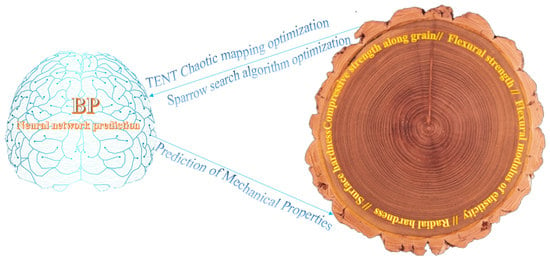
Prediction of Mechanical Properties of Thermally Modified Wood Based on TSSA-BP Model

Abstract

In order to demonstrate whether the sparrow search algorithm can show good performance in optimization, this paper improves the prediction model by this algorithm and predicts the change data of wood mechanical properties under different conditions, which better reflects the connection between the process parameters of wood heat treatment and the change of wood mechanical properties. The article takes the five main mechanical property parameters of thermally modified wood: compressive strength along the grain, flexural strength, flexural elastic modulus, radial hardness, and tangential hardness, respectively, as the objects of study and improves the sparrow search algorithm by Tenting chaotic mapping and then optimizes the Back Propagation (BP) network model by this algorithm. The results show that the number of iterations of the optimized Tent-Sparrow search algorithm-Back Propagation network model (TSSA-BP) is only one-eighth that of the original BP network model, and the convergence speed is greatly improved, the root mean square error of the TSSA-BP model is at least one-half times that of the original BP model, and the optimized model fits the original data better in terms of predicted values; thus, this article provided a feasible prediction algorithm for the field related to the mechanical property changes of wood after heat treatment.

1. Introduction

Wood modification is a cutting-edge research direction in forestry development, and Hill [1] stated that wood modification usually uses chemical, biological, or physical reagents and materials to improve the properties that people demand from wood within a certain service life. Wood modifications include heat treatment, chemical treatment, physical treatment, and treatment based on biological processes on wood. In the past decades, wood modification techniques such as heat treatment have been widely used for wood due to its inherent defects, such as high moisture sensitivity, low dimensional stability, and low resistance to UV and biological attack. In recent years, as the requirements for wood applications have increased, wood modification techniques have also focused on processes that improve the physical, mechanical, or aesthetic properties of the panels [2]. Common heat treatment methods for wood include the traditional Finnish Thermowood method, Dutch Plato Wood method, Rectification heat treatment process in France, the Oil heat Treatment process in Germany, and the Le Bois Perdure process in France, Denmark, and Austria [3]. The mechanism of action of wood modification through the use of heat treatment is that under humid conditions and high temperatures, the acetyl groups of hemicellulose undergo cleavage, and the hemicellulose is hydrolyzed into oligomers and monomeric structures, and the formation of degradation products and oxidation products results in a more attractive wood surface gloss [4]. While the bonds within the lignin complex are cleaved, resulting in a higher concentration of phenolic groups. Esterification occurs in a dry environment and at the right temperature, and the esterification helps to reduce the moisture absorption of the wood, thereby improving its dimensional stability and durability [5]. Different media also have different effects on the heat treatment response of wood. Jianxiong L. et al. [6] conducted a heat treatment of poplar by steam media and established a regression model between color difference, treatment temperature, and time and obtained the conclusion that the color of wood will gradually transition from primary color to dark brown after heat treatment. Sohrab Rahimi et al. [7] compared heat treatments with water and steam media, and they noted that the use of water media causes the degradation of intercellular cavities and wood cells, which can lead to an increase in wood permeability and water absorption, which, in turn, affects the moisture content of the wood, while the use of steam media changes the cell wall structure, which reduces the modulus of elasticity and modulus of rupture of wood samples.

Changes in mechanical properties of wood are related to heat treatment. Bekir Cihad Bal et al. [8] studied the changes in mechanical properties of juvenile and mature wood of Eucalyptus after heat treatment and showed that mechanical properties such as modulus of elasticity, modulus of rupture, compressive strength, and impact bending change significantly in juvenile wood after heat treatment. In addition to heat treatment, the mechanical properties of wood have also been investigated by many other modifications. Antonios N. et al. [9] chemically modified wood by acetic anhydride and found that acetylation significantly affected the toughness of wood. Hadi Y. S. et al. [10] impregnated wood by methyl methacrylate (MMA) and heated it to induce the polymerization process and found that the wood impregnated by MMA was physically and mechanical properties were improved. SH Lee et al. [11] believed that, after oil heat treatment, the equilibrium moisture content of wood decreases, the compressive strength along the grain increases, and the change of mechanical properties brings strong moisture resistance, dimensional stability, and biological durability, which can be applied to floors and outdoor buildings. For the quantitative study of wood properties under thermal modification, in this direction, Hamidreza Fathi [12] used guided Lamb wave propagation and GMDH artificial neural network to discuss the variations of the mechanical properties of wood by guided waves at different wood moisture contents, and the results showed that the Lamb wave velocity is highly sensitive to the mechanical properties of wood, and the experimentally obtained modulus of elasticity and modulus of fracture are more accurate than the data obtained by commonly used methods. Dongyan Z. et al. [13] applied BP networks to wood-drying control research and developed a neural network benchmark model based on wood moisture content prediction. Nasir V. et al. [14] developed a group method of the data handling (GMDII) neural network model with color parameters of western hemlock as input to predict the physical properties such as equilibrium moisture content, density, water absorption, coefficient of expansion, and modulus of elasticity of wood.

Taken together, there have been detailed studies on the changes of wood properties after heat treatment, and many articles even put the prediction of data through realistic instruments to verify the accuracy of the model, such as Fourier-Transform Infrared Spectrometer [5], which is lacking in this study. However, in terms of data prediction, many papers in the wood property prediction literature also used a more single model, less used other algorithmic model comparison, which makes it difficult to discern which is more suitable for the prediction of wood performance, so this paper optimized the algorithmic model twice and then, compared with the original model, can highlight the improvements of the optimization method and the practicality of the optimized model.

2. Mechanical Properties of Wood

Table 1. Raw data of influencing indicators.

Test Temperature/°C	Test Time/h	Test Humidity/%	Compressive Strength along Grain/Mpa	Flexural Strength/Mpa	Flexural Modulus of Elasticity/Gpa	Radial Hardness/Mpa	Tangential Hardness/Mpa
120	0.5	0	39.2	67.4	9.093	14.12	15.56
120	0.5	40	39.1	65.3	9.038	13.02	14.69
120	0.5	60	38.0	69.7	9.1	14.67	15.08
120	0.5	100	36.7	67.2	8.845	14.65	15.45
120	1	0	38.4	67.8	8.649	13.98	14.36
120	1	40	37.6	66.4	8.752	12.98	15.59
120	1	60	38.6	67.8	9.245	13.78	15.32
120	1	100	38.1	63.1	7.895	14.55	14.23
120	2	0	39.5	66.9	9.074	13.33	14.23
120	2	40	38.6	68.2	8.945	12.55	14.58
120	2	60	36.5	65.2	8.854	13.25	14.89
120	2	100	41.9	63.2	8.933	13.36	14.56
120	3	0	37.5	66.5	8.9	13.56	14.78
120	3	40	39.8	67.6	8.963	13.45	14.45
120	3	40	39.8	67.6	8.963	13.45	14.45
120	3	60	37.6	66.6	8.745	13.01	14.69
120	3	100	38.9	64.2	8.745	12.45	14.78
140	0.5	0	36.7	66.7	8.978	14.69	15.56
140	0.5	40	36.9	67.5	8.845	13.06	15.02
140	0.5	60	35.8	66.8	9.155	14.02	14.23
140	0.5	100	38.4	65.3	8.877	15.02	15.01
140	1	0	37.4	66.5	9.179	14.16	15.68
140	1	40	36	64.5	9.137	13.05	15.01
140	1	60	37.2	67.2	9.024	13.49	15.17
140	1	100	37.5	63.1	8.823	13.45	15.48
140	2	0	37.9	66.3	8.823	13.54	14.69
140	2	40	38.5	65.7	8.852	14.69	14.58
140	2	60	37.6	67.1	8.799	13.99	14.74
140	2	100	35.5	62.7	8.9	14.28	15.63
140	3	0	36.9	65.4	8.811	14.39	14.23
140	3	40	38.9	64.6	8.934	13.23	14.56
140	3	60	38.2	65.5	8.654	14.23	13.65
140	3	100	39.2	62.1	8.798	13.56	14.02
160	0.5	0	36.9	66.3	8.788	14.89	14.99
160	0.5	40	39.1	66.9	9.011	14.87	14.36
160	0.5	60	37.1	66.3	8.745	14.58	14.78
160	0.5	100	38.9	65.8	8.712	14.69	15.69
160	1	0	39.1	62.4	8.679	13.42	14.56
160	1	40	39.7	61.4	8.645	14.09	15.3
160	1	60	37.8	62.2	8.798	14.69	15.9
160	1	100	38.7	62.8	8.679	13.58	15.63
160	2	0	35.9	62.2	8.727	14.63	13.92
160	2	40	35.8	62.1	8.557	14.02	14.17
160	2	60	36.6	63.1	8.687	15.17	14.28
160	2	100	38.2	60.9	8.611	14.65	15.09
160	3	0	37.2	61.9	8.611	13.65	14.36
160	3	40	39.1	61.5	8.534	13.47	14.56
160	3	60	39.5	60.8	8.601	13.58	13.89
160	3	100	37.3	60.5	8.552	13.69	14.36
180	0.5	0	38.9	65.9	8.601	15.21	14.03
180	0.5	40	39.1	65.3	8.689	15.98	14.56
180	0.5	60	37.6	66.1	8.645	16.01	13.97
180	0.5	100	36.1	65.7	8.599	14.32	14.33
180	1	0	38.2	65.4	8.623	15.09	13.79
180	1	40	39.4	64.9	8.645	14.98	14.25
180	1	60	37.6	66.3	8.579	15.45	14.08
180	1	100	38.1	64.8	8.545	14.33	13.64
180	2	0	39.5	65.1	8.574	14.65	13.69
180	2	40	38.7	65.8	8.6	14.13	13.59
180	2	09	38.2	64.5	8.532	13.99	14.49
180	2	100	37.1	64.2	8.544	15.1	13.54
180	3	0	38.1	64.1	8.6	14.21	14.06
180	3	40	37.5	64.2	8.541	13.99	14.21
180	3	60	37.8	64.8	8.456	14.58	13.98
180	3	100	38.5	63.8	8.499	14.99	13.69
200	0.5	0	36.5	62.1	8.483	12	13.6
200	0.5	40	35.4	60.6	8.475	11.96	12.99
200	0.5	60	35.1	59.9	8.399	11.45	13.21
200	1	0	34.5	61.9	8.422	11.69	12.98
200	1	40	35.8	60.8	8.489	11.46	12.64
200	1	60	34.1	61.2	8.321	11.54	12.35
200	2	0	34.6	61.2	8.369	11.99	13.02
200	2	40	35.4	60.8	8.354	11.15	12.69
200	2	60	34.5	60.5	8.211	10.65	12.49
200	3	0	34.1	60.9	8.249	10.68	12.73
200	3	40	34.2	59.8	8.231	11.05	12.57
200	3	60	33.8	58.2	8.011	10.22	12.37
210	0.5	0	34.1	50.1	7.856	10.23	10.98
210	0.5	40	33.2	50.8	7.789	10.59	9.98
210	0.5	60	32.1	49.9	7.865	10.55	10.23
210	1	0	33.9	50.6	7.765	10.21	10.65
210	1	40	32.9	49.8	7.712	9.98	10.21
210	1	60	32.8	48.9	7.498	10.01	10.65
210	2	0	32.9	49.1	7.689	9.98	9.64
210	2	40	32.5	49.5	7.712	9.65	9.35
210	2	60	31.8	49.6	7.623	10.03	9.67
210	3	0	31.5	47.8	7.5	9.21	8.91
210	3	40	30.5	46.5	7.412	9.1	8.21
210	3	60	30.8	45.1	7.321	9.03	8.99

shows the experimental data, which are based on experiments by HongY. et al. [15] and are publicly available in Bioresource at http://doi.org/10.15376/biores.10.3.5758-5776, accessed on 25 October 2021.

The experiments were carried out on Larix gmelini with 22-mm thickness for the heat treatment, and the ambient temperature was set at 20 °C, and the relative humidity was 65%. The mechanical properties of the wood were tested in strict accordance with Chinese national standards. The control variables for wood heat treatment were temperature, humidity, and time, and a total of 88 sets of experimental data were obtained.

The heat treatment experiment goes through three stages. Firstly, the experimental wood is preheated by saturated steam under the instrument. By setting the high temperature and corresponding pressure, the moisture content of the wood in this stage is nearly zero. Secondly, the wood is protected by steam, and the heat treatment process is carried out under the high-temperature and high-pressure tank. Finally, the instrument is depressurized, and the wood is cooled to prevent dry cracking of the wood.

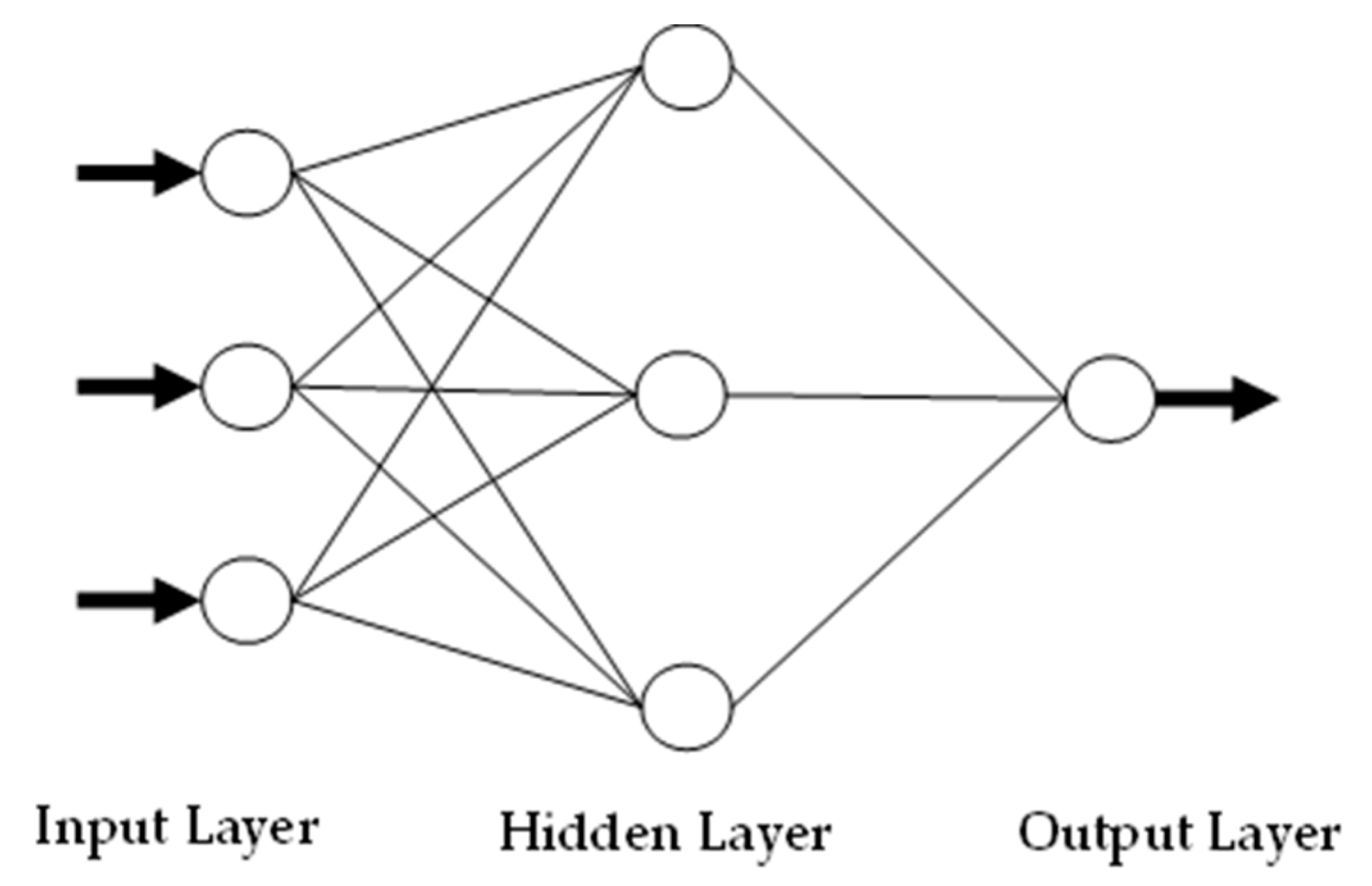
3. Establishment of BP Neural Network Model

3.1. Determination of Node Number of Input Layer and Output Layer

As a multilayer feed-forward neural network, the BP neural network can simulate human brain nerves for error correction. The BP neural network first propagates the signal from the input layer through the implicit layer and finally reaches the output layer for forward propagation and then transmits the error back to the input layer in reverse after comparing with the actual data and adjusts the weights and biases of each layer in turn.

After building the neural network structure as shown in Figure 1 according to the neural network principle, the model takes the three input nodes of temperature, humidity, and time as the input layer data, and then takes the wood mechanical properties as the output layer data, i.e., one output node, respectively. Since the input metrics are three-dimensional and the output metrics are one-dimensional; the number of input nodes for BP is 3 and the number of output nodes is 1, as shown in Figure 2 below.

In order to ensure the effectiveness of neural network, 88 groups of experimental data in Table 1 are divided into training set and verification set. Fifty-eight groups of data are used as the training set, and 30 groups of data are used as the verification set, which are brought into MATLAB operations. In this paper, all functions are set by the MATLAB machine learning toolbox; here, the neural network activation function is the Sigmoid function, and the training algorithm is the gradient descent method. The mechanical properties of wood after thermal modification are predicted by the BP neural network prediction model to test the prediction effect of BP neural network model.

3.2. Determination of Number of Hidden Layer Nodes

The nodes of the hidden layer of the BP neural network are calculated by assuming that the number of input nodes is m, and the number of output nodes is n. The optimal value of the number of nodes of the hidden layer falls in the range of $\sqrt{m+n}$ + a, with a being any number between 1 and 10. In this experiment, the number of input nodes is 3, and the number of output nodes is 1. Therefore, the number of hidden layer nodes is designed to range from 3 to 12. By comparing the mean square error between the predicted value and the actual value of the training set corresponding to the number of hidden layer nodes, the number of hidden layer nodes with the smallest mean square error is the best case. Taking the diameter tangential hardness of wood as an example, the results are shown in

Table 2. Implied layer nodes and simulation errors.

Number of Hidden Layer Nodes	Mean Square Error of Training Set Simulation
3	0.076652
4	0.080913
5	0.11162
6	0.098472
7	0.11095
8	0.20944
9	0.048599
10	0.10292
11	0.053805
12	0.080683

below. The value with the smallest mean square error is the best implied node, and the best number of implied layer nodes is 9 from Table 2, and the corresponding mean square error is 0.048599.

After the BP network model iteration, the corresponding error rate of the model can be calculated, as shown in

Table 3. BP model error.

Error	BP Model Error Data
Mean absolute error	3.1008
Mean square error	11.7437
root mean square error	3.4269
Mean absolute percentage error	29.4895%

.

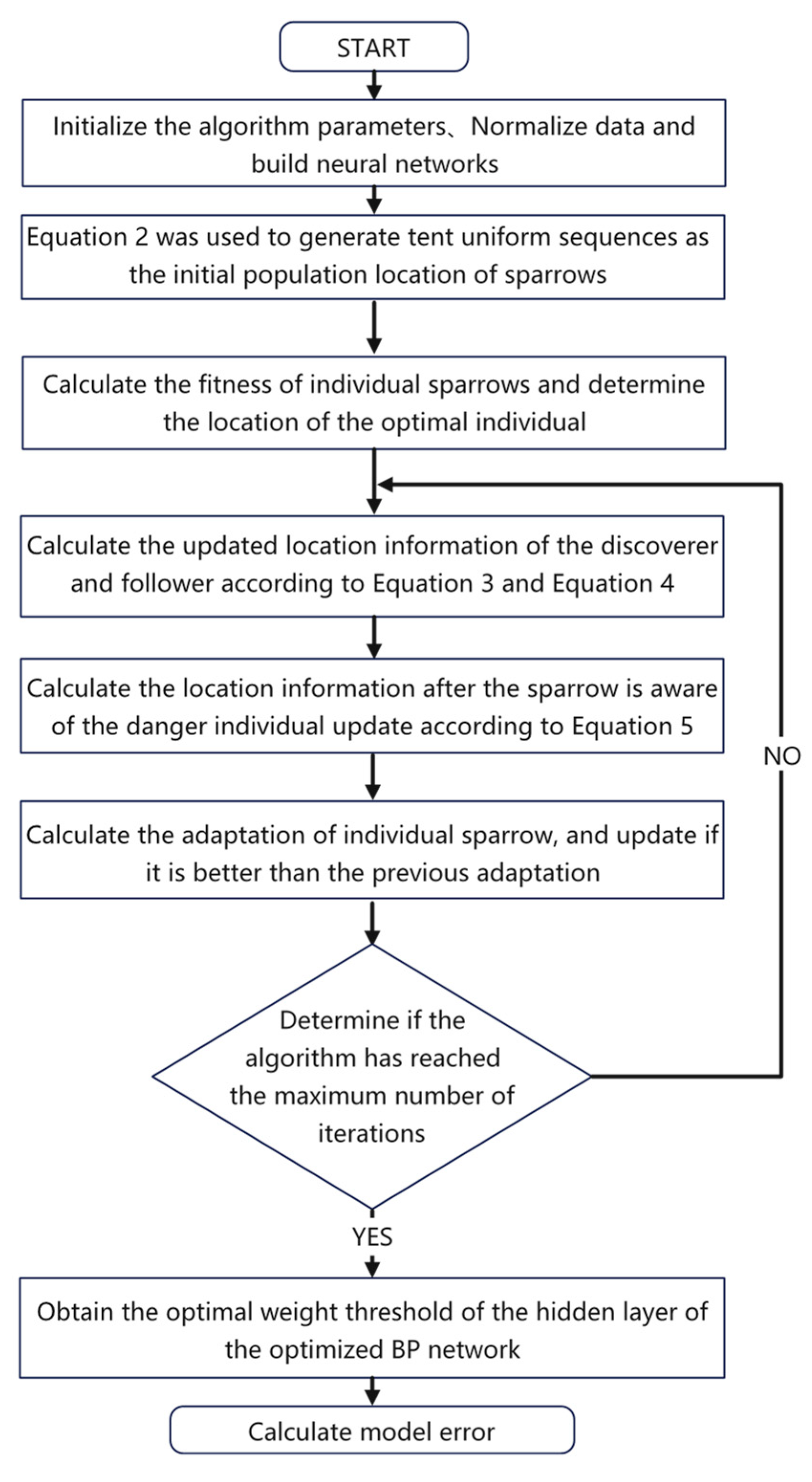
4. Establishment of TSSA Model

4.1. Tent Chaotic Mapping

Chaotic mapping is often used to solve the problem that some heuristic algorithms tend to fall into local optimum. Chaotic mapping originates from chaotic phenomenon, i.e., there may be some unpredictable variables in a certain system. By adding unknown variables in heuristic algorithm to improve the accuracy of algorithm through the principle of chaotic phenomenon, it can improve the link of global search and get rid of local optimal limit [16].

Tent chaotic mapping function can uniformly generate chaotic sequence in (0, 1) interval, as shown in Formula (1).

$${{\displaystyle x}}_{i+1}=\{\begin{array}{c}2x,0\le x_i\le \frac{1}{2}\\ 2(1-x_i),\frac{1}{2}\le x_i\le 1\end{array}$$

(1)

The chaotic sequence generated by the chaotic operator is more likely to fall into the unknown periodic point due to its periodicity during iteration, so the random variable rand function can be added to make it stable. The Tent operator needs to have the ability to handle large amounts of data through Bernoulli’s change, and Formula (2) is obtained, where N is the number of particles in the sequence.

$$x_{i+1}=(2x_i)\mathrm{mod}1+rand(0,1)\ast \frac{1}{N}$$

(2)

The Tent chaos algorithm is widely used in the optimization of heuristic algorithms, such as Kuang F. J. et al. [17] replacing the randomly generated initial population in the artificial bee colony algorithm with a Tent chaos sequence to improve its convergence speed. Xu W. H. et al. [18] coevolved the artificial bee colony algorithm optimized by Tent chaos mapping with the particle swarm algorithm to avoid the defect that the original algorithm stopped iterating too early.

4.2. Sparrow Search Algorithm

The sparrow search algorithm is a heuristic algorithm proposed by Xue Jiankai et al. [19] in 2020, which simulated the behavior of sparrows in nature. The algorithm divided the behavior of sparrows foraging into three categories. The individual searching for food is the discoverer, and the rest is the follower. The sparrow individual will change its identity according to the special circumstances, such as the dangerous situation while foraging [20]. At the same time, the sparrow also has the identity of a guard. When the danger is discovered, the sparrow will give up in time, or monitor whether the same kind has the behavior of fighting for food during foraging [21].

In the sparrow search algorithm, assuming that the initial population size of the sparrow race is n, the position of each individual in the D-dimensional space is $X=\left(x_1,x_2,x_3,\dots x_D\right)$, and the d-dimensional position of the ith sparrow individual in the iteration t is expressed as $x_{i,d}^{t+1}$, N is a random number conforming to the standard normal distribution, $R_2\in \left[0,1\right]$, which represents the warning random number of the alert person encountering danger, and $ST\in \left[0,1\right]$ is the alert threshold value. When $R_2$ it is greater than ST, the individual of the discoverer will randomly transfer to the current position according to the normal distribution; that is, the sparrow will transfer to the foraging place if the threshold value is exceeded. The finder position for each iteration is shown in Formula (3).

$$x_{i,d}^{t+1}=\{\begin{array}{c}{x}_{i,d}^t\ast (1+N)\\ x_{i,d}^t+N\end{array}\begin{array}{c},R_2<ST\\ ,R_2\ge ST\end{array}$$

(3)

In addition to the sparrow individuals of the discoverer and the watchman, the remaining individuals are temporarily followers, and the discoverers are foraging, thus creating a matrix representing followers randomly from {−1, 1} for each dimension. xw is $x_{worst}$, which represents the current worst sparrow position, xb is $x_{best},$ which represents the current optimal sparrow position. In the sparrow predation rule, the follower will follow the discoverer with the best position to search for food more efficiently. If $i\le \frac{n}{2}$, the discoverer finds the food at the earliest and finds the food at the end, and the follower will choose to go to the unexplored area to search for food later. The follower position update formula is shown in Equation (4).

$${{\displaystyle x}}_{i,d}^{t+1}=\{\begin{array}{c}N\ast \exp \left(\frac{x{w}_{i,d}^t-x_{i,d}^t}{i^2}\right)\\ x{b}_{i,d}^t+\frac{1}{D}{\displaystyle \sum _{d=1}^D(rand\{-1,1\}\ast (\left|x{b}_{i,d}^t-x_{i,d}^t\right|))}\end{array}\begin{array}{c},i>\frac{n}{2}\\ ,i\le \frac{n}{2}\end{array}$$

(4)

The alert person will judge whether the environment is dangerous when the sparrow is foraging. If so, the current food will be abandoned, and the whole population will be transferred. Since each individual has no fixed identity, the individual will be randomly selected as the alert person in each iteration. If the guard is in the nonoptimal position, the guard will move to the random position between the current position and the optimal position if the guard escapes to a random position between the optimal position and the worst position when the guard is in the optimal position. If $f_i\ne f_g$, the guard will be vulnerable to attack in the periphery of the population; otherwise, the guard will approach the companion, where $\beta$ is a random number with a normal distribution. The alert position update formula is shown in Equation (5).

$$x_{i,d}^{t+1}=\{\begin{array}{c}{x}_{i,d}^t+\beta \ast (x_{i,d}^t-x{b}_{i,d}^t)\\ x_{i,d}^t+\beta \ast (x{w}_{i,d}^t-x{b}_{i,d}^t)\end{array}\begin{array}{c},f_i\ne f_g\\ ,f_i=f_g\end{array}$$

(5)

4.3. TSSA-BP Model

The sparrow search algorithm is a process in which the predation behavior of sparrow is compared with that of the algorithm to find the optimal solution, the dimensional information of sparrow in predation is taken as the search node of the algorithm, the fitness of sparrow in predation is taken as the solution of the objective function, and the predation process is compared with the iterative optimal solution process in the optimization process [22]. The original Sparrow search algorithm is easy to fall into the local optimal situation after the warner transfers the optimal position, and the algorithm has the limitations of slow convergence speed and low accuracy. Therefore, the Tent chaotic mapping is used to add a random sequence to improve the accuracy of the SSA algorithm, The model is named TSSA. The ergodicity of chaotic mapping can give the initial population diversity of sparrow and improve its convergence speed and wide area search ability.

The operational flow chart of the BP model improved by TSSA is shown in Figure 3 below. First, the data need to be normalized, and thus, the data layers are divided to construct the initial neural network. Then, initialize the parameters, such as warning value R, safety value ST, etc. Then, a chaotic sequence is generated using the Tent chaos mapping as a way to represent the initial position of the sparrow population. According to Equations (3)–(5), discoverers, followers, and warners of the sparrow population can be generated. Finally, $x_{worst}$ and $x_{best}$ are determined by the fitness of each individual, and if a better individual fitness cannot be obtained, the algorithm is judged to reach the maximum value, and the hidden layer weights of the neural network are obtained when the number of iterations is optimal.

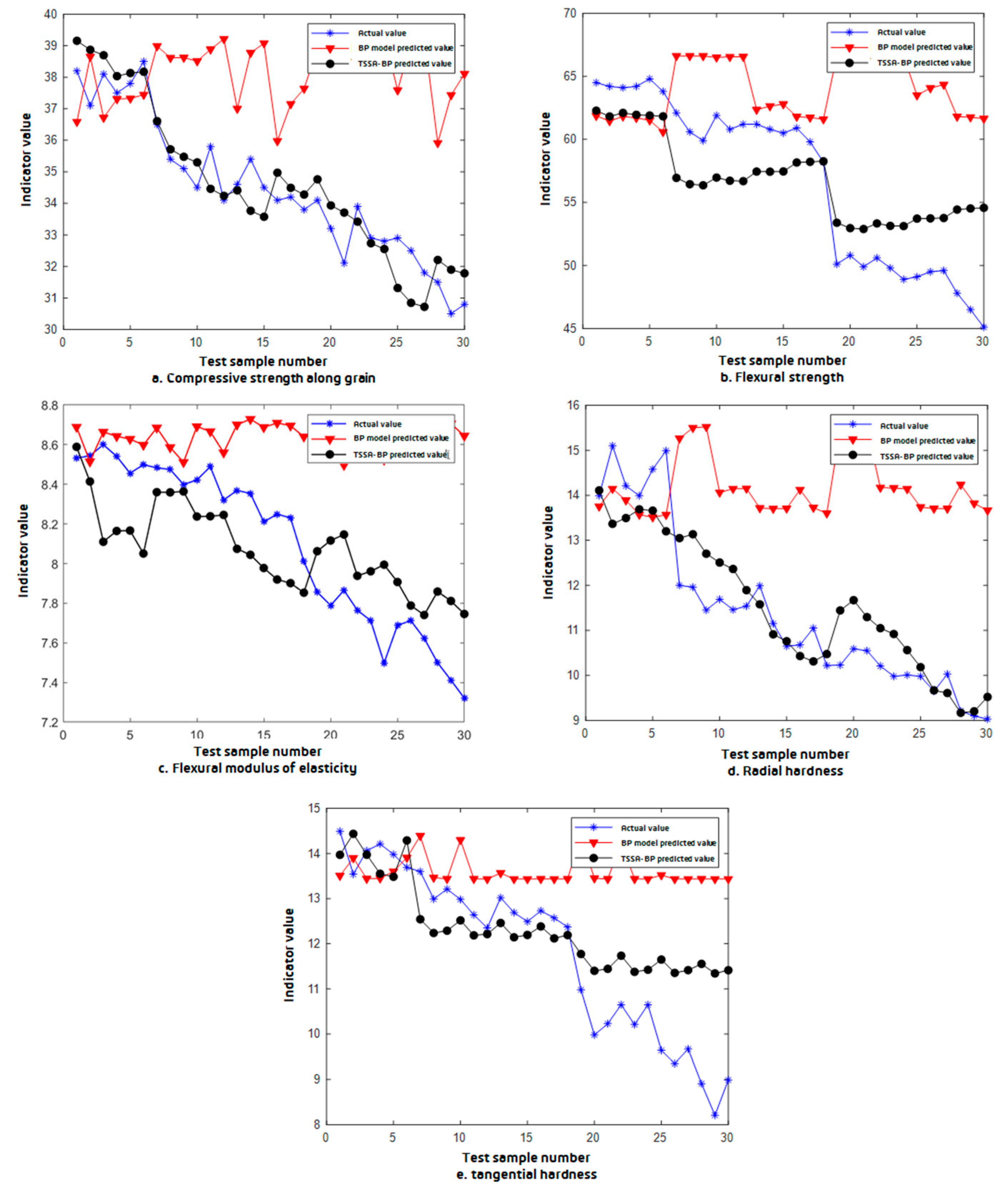
5. Results and Discussion

The accuracy of the model can be judged by the error rate, and the common statistical errors include the mean absolute error (MAE), the mean square error(MSE), the root mean square error (RMSE), and the mean absolute percentage error (MAPE), where the root mean square error (RMSE) is the square root of the ratio of the square of the deviation between the predicted value and the real value and the observation number, which can be used to measure the dispersion degree of a group of numbers themselves and can better reflect the actual situation of the predicted value error. RMSE ∈ [0, +∞); when the predicted value and the real value are completely consistent, RMSE is equal to 0; that is, the perfect model, and the greater the error, the greater the value. As shown in

Table 4. BP model and error quantity.

	BP Neural Network				TSSA-BP Neural Network
	MAE	MSE	RMSE	MAPE	MAE	MSE	RMSE	MAPE
Compressive Strength along Grain	3.0589	15.2339	3.9031	9.23%	1.0031	1.4796	1.2164	2.90%
Flexural Strength	8.3386	108.3442	10.4089	16.19%	3.6837	16.9941	4.1224	6.81%
Flexural Modulus of Elasticity	281.1056	2,359,375	1536.026	11.84%	282.5553	2,357,955	1535.563	31.26%
Radial Hardness	3.1008	11.7437	3.4269	29.49%	0.65949	0.66027	0.81257	5.64%
Tangential Hardness	1.9485	6.3025	2.5105	19.12%	0.9944	1.5728	1.2541	9.61%

below, the RMSE values of the TSSA-BP model for mechanical property prediction are all much smaller than those of the BP model, indicating that the optimized model shows good results.

The prediction effect of the model can also be observed through the line chart. Figure 3 shows the comparison of the predicted values of the five mechanical properties under the BP model and the TSSA-BP model. Taking the diameter radial hardness of wood as an example, as shown in Figure 4d below, the BP model fluctuates greatly and has a high error with the original data, while the TSSA-BP model can better fit the original data and achieve a low error with the original data after a certain amount of training. Setting the maximum number of iterations of the model to 1000, the BP model is iterated 65 times, and the TSSA-BP model is iterated eight times, which shows that the optimization model has obvious advantages in convergence speed.

In this paper, predictions of five mechanical properties of wood after heat treatment were made, but according to the results, the modulus of elasticity did not fit well into the predictions of the model and could not reflect a high expressiveness in the model. In addition to this, there are a wide range of mechanical properties of wood, and in subsequent studies, it might be appropriate to consider some algorithm to determine which mechanical properties are more representative of wood properties or more suitable for model prediction; for example, Nasir V et al. [14] used an equilibrium of moisture content, density, porosity, water absorption, swelling coefficient, dynamic modulus of elasticity, and hardness as model predictors, and these keywords are worthy of reference. The more indicators are more responsive to the relationship between heat treatment and the relationship between mechanical property changes, but more indicators also affect the accuracy of the model, so irrelevant or redundant input features can be removed through feature selection [23]. In terms of data selection, because the original experiment has taken the arithmetic mean of three parallel experiments for each group of experimental data to avoid large bias [15], and although data partitioning can effectively improve the performance of the model, data partitioning is of little help in explaining the model, so data partitioning is not performed on the data in this paper, which will be a point of attention to continue optimizing the model in the future. Through the existing literature data and error rate judgment, we tentatively believe that the optimization model has a higher accuracy rate than some other algorithms; for example, M. Schubert et al. [24] also conducted a model error calculation of RMSE for compressive strength, and the result was 17.19, while the result of the TSSA-BP model was 3.90. This comparison result was affected by the sample size, and the processing parameters might not have been accurate, but in conditions permitting, further research can be done in the future. In addition, this paper not only adopted the newly born sparrow search algorithm in 2020 but also adopted the Tent chaos mapping optimization model in order to compensate for the disadvantage that the heuristic algorithm tends to stop iterating too early. Taken together, the TSSA-BP-based optimization model has been able to predict the relevant properties of wood after heat treatment more accurately, which provides help to better control the process parameter variables in subsequent heat treatment studies.

6. Conclusions

Changes in heat treatment parameters are apparently highly correlated with the mechanical properties of the wood, and the predictability is shown as follows: Compressive Strength along Grain > Radial Hardness > Flexural Modulus of Elasticity > Tangential Hardness > Flexural Strength. Tangential Hardness and Flexural Strength are related to the density of the wood, while the density-dependent properties do not perform well for predictions, which can initially reflect that the change in wood density after heat treatment is not significant. The most relevant wood property for heat treatment is the color brightness of the wood skin, which can be used as an important predictive parameter in future related studies. A predicted performance can also improve the utilization in the industry for lumber processing, for example, mills can consider how to cut wood in a radial or tangential direction to maximize the use of the current physical properties of the wood. The comparison of the model prediction values verified that chaotic operators help inspiring algorithms to avoid easy access to the local optima, providing a viable idea for future research in related algorithm areas and thus reducing the algorithm trial and error and improving the research efficiency.

References

1. Callum, A.S.H. Wood Modification: Chemical, Thermal and Other Processes; John Wiley & Sons: Chichester, UK, 2006; pp. 260–262. [Google Scholar] [CrossRef]
2. Sandberg, D.; Kutnar, A.; Mantanis, G. Wood modification technologies—A review. iFor.-Biogeosci. For. 2017, 10, 895–908. [Google Scholar] [CrossRef] [Green Version]
3. Dong, X.; Jianpeng, H.; Lihong, Y. Research status and development of wood property prediction and quality control of heat treated wood. J. Zhejiang Agrofor. Univ. 2020, 37, 1–8. [Google Scholar] [CrossRef]
4. Dubey, M.K.; Pang, S.; Walker, J. Changes in chemistry, color, dimensional stability and fungal resistance of Pinus radiata D. Don wood with oil heat-treatment. Holzforsch 2012, 66, 49–57. [Google Scholar] [CrossRef]
5. Tjeerdsma, B.F.; Militz, H. Chemical changes in hydrothermal treated wood: FTIR analysis of combined hydrothermal and dry heat-treated wood. Holz Als Roh-Und Werkst. 2005, 63, 102–111. [Google Scholar] [CrossRef]
6. Lu, J.; Huang, R.; Cao, Y.; Wu, Y.; Zhou, Y.; Zhao, Y.; Wu, Y. Effect of Steam Heat Treatment on Color of Chinese White Poplar Wood. Sci. Silvae Sin. 2012, 48, 126–130. [Google Scholar] [CrossRef]
7. Rahimi, S.; Singh, K.; DeVallance, D. Effect of Different Hydrothermal Treatments (Steam and Hot Compressed Water) on Physical Properties and Drying Behavior of Yellow-Poplar (Liriodendron tulipifera). For. Prod. J. 2019, 69, 42–52. [Google Scholar] [CrossRef]
8. Bal, B.C.; Bektaş, I. The Effects of Heat Treatment on Some Mechanical Properties of Juvenile Wood and Mature Wood ofEucalyptus grandis. Dry. Technol. 2013, 31, 479–485. [Google Scholar] [CrossRef]
9. Papadopoulos, A.N.; Tountziarakis, P. Toughness of pine wood chemically modified with acetic anhydride. Eur. J. Wood Wood Prod. 2012, 70, 399–400. [Google Scholar] [CrossRef]
10. Hadi, Y.S.; Massijaya, M.Y.; Zaini, L.H.; Pari, R. Physical and Mechanical Properties of Methyl Methacrylate-Impregnated Wood from Three Fast-Growing Tropical Tree Species. J. Korean Wood Sci. Technol. 2019, 47, 324–335. [Google Scholar] [CrossRef]
11. Lee, S.H.; Ashaari, Z.; Lum, W.C.; Halip, J.A.; Ang, A.F.; Tan, L.P.; Chin, K.L.; Tahir, P.M. Thermal treatment of wood using vegetable oils: A review. Constr. Build. Mater. 2018, 181, 408–419. [Google Scholar] [CrossRef]
12. Fathi, H.; Nasir, V.; Kazemirad, S. Prediction of the mechanical properties of wood using guided wave propagation and machine learning. Constr. Build. Mater. 2020, 262, 120848. [Google Scholar] [CrossRef]
13. Dongyan, Z. Neural Network Prediction Model of Wood Moisture Content for Drying Process. Sci. Silvae Sin. 2008, 44, 94–98. [Google Scholar] [CrossRef]
14. Nasir, V.; Nourian, S.; Avramidis, S.; Cool, J. Prediction of physical and mechanical properties of thermally modified wood based on color change evaluated by means of “group method of data handling” (GMDH) neural network. Holzforsch 2019, 73, 381–392. [Google Scholar] [CrossRef]
15. Yang, H.; Cheng, W.; Han, G. Wood Modification at High Temperature and Pressurized Steam: A Relational Model of Mechanical Properties Based on a Neural Network. Bioresources 2015, 10, 5758–5776. [Google Scholar] [CrossRef]
16. Bing, L.; Weisun, J. Chaos optimization method and its application. Control Theory Appl. 1997, 14, 613–615. Available online: https://en.cnki.com.cn/Article_en/CJFDTotal-KZLY199704028.htm (accessed on 25 October 2021).
17. Kuang, F.J.; Xu, W.H.; Jin, Z. Artificial bee colony algorithm based on self-adaptive Tent chaos search. Control Theory Appl. 2014, 11, 1502–1509. [Google Scholar] [CrossRef]
18. Williams, A.; Langridge, H.; Straathof, A.L.; Muhamadali, H.; Hollywood, K.A.; Goodacre, R.; de Vries, F.T. Hybridization algorithm of Tent chaos artificial bee colony and particle swarm optimi-zation. Control Decis. 2015, 30, 839–847. [Google Scholar] [CrossRef]
19. Xue, J.; Shen, B. A novel swarm intelligence optimization approach: Sparrow search algorithm. Syst. Sci. Control Eng. 2020, 8, 22–34. [Google Scholar] [CrossRef]
20. Barta, Z.; Liker, A.; Mónus, F. The effects of predation risk on the use of social foraging tactics. Anim. Behav. 2004, 67, 301–308. [Google Scholar] [CrossRef]
21. Bautista, L.M.; Alonso, J.C.; A Alonso, J. Foraging site displacement in common crane flocks. Anim. Behav. 1998, 56, 1237–1243. [Google Scholar] [CrossRef] [Green Version]
22. Jingyu, H. Research on Sparrow Search Algorithm Combining t-Distribution and Tent Chaotic Mapping. Master’s Thesis, Lanzhou University, Lanzhou, China, 21 May 2021. [Google Scholar] [CrossRef]
23. Cai, J.; Luo, J.; Wang, S.; Yang, S. Feature selection in machine learning: A new perspective. Neurocomputing 2018, 300, 70–79. [Google Scholar] [CrossRef]
24. Schubert, M.; Luković, M.; Christen, H. Prediction of mechanical properties of wood fiber insulation boards as a function of machine and process parameters by random forest. Wood Sci. Technol. 2020, 54, 703–713. [Google Scholar] [CrossRef]
Figure 1. BP Network Structure.
Forests 13 00160 g001
Figure 2. Determination of the node number of input layer and output layer.
Forests 13 00160 g002
Figure 3. TSSA-BP model flow chart.
Forests 13 00160 g003
Figure 4. Comparison between the predicted and actual values of the BP neural network before and after TSSA optimization.
Forests 13 00160 g004