
Past Disturbance–Present Diversity: How the Coexistence of Four Different Forest Communities within One Patch of a Homogeneous Geological Substrate Is Possible


Abstract
:1. Introduction
1.1. Soil Conditions and Disturbance as Factors Influencing Forest Ecosystems
1.2. Influence of Land Use Change on Oligotrophic Forest Dynamics and Forest Conservation in Central Europe
1.3. Aim
2. Materials and Methods
2.1. Study Site
2.2. Fieldwork
2.3. Laboratory Analysis
2.4. Data Preparation and Analysis
2.4.1. Data Preparation
2.4.2. Data Analysis
3. Results
4. Discussion
4.1. Predictive Variables
4.2. From Psammophilous Grasslands, through Cladonia-Scots Pine Forest, to Acidophilous Oak Forest—Uniquely Diverse Vegetation within Initially Homogenous Psammophilous Conditions
4.3. Historic Soil Disturbance by Tillage Explains the Present Diversity of Vegetation
4.4. Implications for Forest Management and Conservation
4.4.1. Implications for Nature Conservation
4.4.2. Implications to Forest Management
5. Conclusions
- Past soil disturbance resulting from tillage is the main factor enhancing the diversity of forest communities in the oligotrophic fluvioglacial site.
- The presence of two protected forest EU Natura 2000 habitat types, which need different management methods, may require choosing, whether to protect transitional and anthropogenic Cladonia-Scots pine forest (code 91T0) or late-successional acidophilous oak forest (code: 9190). Management decisions will be more concerned with the fate of lichen-rich pine forests.
- It may be necessary to reassess management plans and conservation decisions when considering forests on oligotrophic-sandy substrates.
- Post-agricultural Brunic Arenosols that are lightly degraded appear to promote oak establishment, while medium soil disturbance favors pine plantations.
- Near complete soil-profile denudation can be used as an indicator of potential sites for Cladonia-Scots pine forest conservation.
- The potential natural vegetation of the study site differs from potentially restorable vegetation: the PNV of pine forest is still pine forests, the PNV of oak–pine forest and acidophilous oak forest is acidophilous oak forest, and the PRV of the entire study site is acidophilous oak forest.
Supplementary Materials
Author Contributions
Funding
Institutional Review Board Statement
Informed Consent Statement
Data Availability Statement
Acknowledgments
Conflicts of Interest
References
- Peterken, G.F. Natural Woodland, Ecology and Conservation in Northern Temperate Regions; Cambridge University Press: Cambridge, UK, 1996. [Google Scholar]
- Shorohova, E.; Kuuluvainen, T.; Kangur, A.; Jõgiste, K. Natural stand structures, disturbance regimes and successional dynamics in the Eurasian boreal forests: A review with special reference to Rusian studies. Ann. For. Sci. 2009, 66, 201. [Google Scholar] [CrossRef] [Green Version]
- Härdtle, W.; von Oheimb, G.; Westphal, C. Relationships between the vegetation and soil conditions in beech and beech-oak forests of northern Germany. Plant Ecol. 2005, 177, 113–124. [Google Scholar] [CrossRef]
- Neri, A.V.; Schaefer, C.E.G.R.; Silva, A.F.; Souza, A.L.; Ferreira-Junior, W.G.; Meira-Neto, J.A.A. The influence of soil conditions on the floristic composition and community structure of an area of Brazilian Cerrado vegetation. Edinb. J. Bot. 2012, 69, 1–27. [Google Scholar] [CrossRef]
- Zhang, C.; Li, X.; Chen, L.; Xie, G.; Liu, C.; Pei, S. Effects of Topographical and Edaphic Factors on Tree Community Structure and Diversity of Subtropical Mountain Forests in the Lower Lancang River Basin. Forests 2016, 7, 222. [Google Scholar] [CrossRef]
- Higgins, M.A.; Roukolainen, K.; Tuomisto, H.; Llerena, N.; Cardenas, G.; Phillips, O.L.; Vásquez, R.; Räsänen, M. Geological control of floristic composition in Amazonian forests. J. Biogeogr. 2011, 38, 2136–2149. [Google Scholar] [CrossRef] [PubMed] [Green Version]
- Reczyńska, K.; Pech, P.; Świerkosz, K. Phytosociological Analysis of Natural and Artificial Pine Forests of the Class Vaccinio-Piceetea Br.-Bl. in Br.-Bl. et al. 1939 in the Sudetes and Their Foreland (Bohemian Massif, Central Europe). Forests 2021, 12, 98. [Google Scholar] [CrossRef]
- Zwydak, M.; Lasota, J.; Brożek, S.; Wanic, T. Różnorodność gleb zespołów borów sosnowych. Rocz. Glebozn. 2011, 62, 39–53. [Google Scholar]
- Lasota, J. Siedliskowo-florystyczna analiza środkowoeuropejskiego acydofilnego lasu dębowego (Calamagrostio arundinaceae-Quercetum petraeae [Hatm. 1934], Scam.et Pass. 1959). Zesz. Nauk. UR im. Hugona Kołłątaja w Krakowie 2013, 393, 5–143. [Google Scholar]
- Sewerniak, P. Differences in early dynamics and effects of slope aspect between naturally regenerated and planted Pinus sylvestris woodland on inland dunes in Poland. iForest 2016, 9, 875–882. [Google Scholar] [CrossRef] [Green Version]
- Danneyrolles, V.; Dupuis, S.; Fortin, G.; Leroyer, M.; de Römer, A.; Terrail, R.; Vellend, M.; Boucher, Y.; Laflamme, J.; Bergeron, Y.; et al. Stronger influence of anthropogenic disturbance than climate change on century-scale compositional changes in northern forests. Nat. Commun. 2019, 10, 1265. [Google Scholar] [CrossRef]
- Kaplan, J.O.; Krumhardt, K.M.; Zimmermann, N. The prehistoric and preindustrial deforestation of Europe. Quat. Sci. Rev. 2009, 28, 3016–3034. [Google Scholar] [CrossRef]
- Halpern, M.T.; Whalen, J.K.; Madramootoo, C.A. Long-term tillage and residue management influences soil C and N dynamics. Soil Sci. Soc. Am. J. 2010, 74, 1211–1217. [Google Scholar] [CrossRef]
- Van Eerd, L.L.; Congreves, K.A.; Hayes, A.; Verhallen, A.; Hooker, D.C. Long-term tillage and croprotation effects on soil quality, organic carbon, and total nitrogen. Can. J. Soil Sci. 2014, 94, 303–315. [Google Scholar] [CrossRef]
- Kobierski, M.; Cieścińska, B.; Cieściński, J.; Kondrakiewicz-Maciejewska, K. Effect of Soil Management Practices on the Mineralization of Organic Matter and Quality of Sandy Soils. J. Ecol. Eng. 2020, 21, 217–223. [Google Scholar] [CrossRef]
- Kazlauskaite-Jadzevice, A.; Tripolskaja, L.; Volungevicius, J.; Baksiene, E. Impact of land use change on organic carbon sequestration in Arenosol. Agric. Food Sci. 2019, 28, 9–17. [Google Scholar] [CrossRef]
- Van Oost, K.; Govers, G.; de Alba, S.; Quine, T.A. Tillage erosion: A review of controlling factors and implications for soil quality. PPG Earth Environ. 2006, 30, 443–466. [Google Scholar] [CrossRef] [Green Version]
- Świtoniak, M. Use of soil profile truncation to estimate influence of accelerated erosion on soil cover transformation in young morainic landscapes, North-Eastern Poland. Catena 2014, 116, 173–184. [Google Scholar] [CrossRef]
- Sewerniak, P.; Jankowski, M.; Dąbrowski, M. Effect of topography and deforestation on regular variation of soils on inland dunes in the Toruń Basin (N Poland). Catena 2017, 149, 318–330. [Google Scholar] [CrossRef]
- Winkler, K.; Fuchs, R.; Rounsevell, M.; Herold, M. Global land use changes are four times greater than previously estimated. Nat. Commun. 2021, 12, 2501. [Google Scholar] [CrossRef]
- Plieninger, T.; Draux, H.; Fagerholm, N.; Bieling, C.; Bürgi, M.; Kizos, T.; Kuemmerle, T.; Primdahl, J.; Verburg, P.H. The driving forces of landscape change in Europe: A systematic review of the evidence. Land Use policy 2016, 57, 204–214. [Google Scholar] [CrossRef] [Green Version]
- Ustaoglu, E.; Collier, M.J. Farmland abandonment in Europe: An overview of drivers, consequences, and assessment of the sustainability implications. Environ. Rev. 2018, 26, 396–416. [Google Scholar] [CrossRef]
- Prah, K.; Řehounková, K.; Lencová, K.; Jírova, A.; Konvalinková, P.; Mudrák, O.; Študent, V.; Vaněček, Z.; Tichý, L.; Petřík, P.; et al. Vegetation succession in restoration of disturbed sites in Central Europe: The direction of succession and species richness across 19 seres. Appl. Veg. Sci. 2014, 17, 193–200. [Google Scholar] [CrossRef]
- Sewerniak, P. Survey of some attributes of post-agricultural lands in Polish State Forests. Ecol. Quest. 2015, 22, 9–16. [Google Scholar] [CrossRef] [Green Version]
- Rahmonov, O. Relacje Między Roślinnością i Glebą w Inicjalnej Fazie Sukcesji na Obszarach Piaszczystych; Prace Naukowe Uniwersytetu Śląskiego w Katowicach 2506; Wydawnictwo Uniwersytetu Śląskiego: Katowice, Poland, 2007. [Google Scholar]
- Prah, K.; Ujházy, K.; Knopp, V.; Fanta, J. Two centuries of forest succession, and 30 years of vegetation changes in permanent plots in an inland sand dune area, The Netherlands. PLoS ONE 2021, 16, e0250003. [Google Scholar] [CrossRef]
- Brzeziecki, B.; Pommerening, A.; Miścicki, S.; Drozdowski, S.; Żybura, H. A Common Lack of Demographic Equilibrium among Tree Species in Białowieża National Park (NE Poland): Evidence from Long-Term Plots. J. Veg. Sci. 2016, 27, 460–469. [Google Scholar] [CrossRef]
- Brzeziecki, B.; Woods, K.; Bolibok, L.; Zajączkowski, J.; Drozdowski, S.; Bielak, K.; Żybura, H. Over 80 years without major disturbance, late-succesional Białowieża woodlands exhibit complex dynamism, with coherent compositional shifts towards true old-growth conditions. J. Ecol. 2020, 108, 1138–1154. [Google Scholar] [CrossRef]
- Benayas, J.M.; Martins, A.; Nicolau, J.M.; Schulz, J.J. Abandomnent of agricultural land: An overview of drivers and consequences. CAB Rev. Perspect. Agric. Vet. Sci. Nutr. Nat. Resour. 2007, 2, 057. [Google Scholar] [CrossRef] [Green Version]
- Mantero, G.; Morresi, D.; Marzano, R.; Motta, R.; Mladenoff, D.J.; Garbarino, M. The influence of land abandonment on forest disturbance regimes: A global review. Landsc. Ecol. 2020, 35, 2723–2744. [Google Scholar] [CrossRef]
- Jakubowska-Gabara, J. Decline of Potentillo albae-Quercetum Libb. 1933 Phytocoenoses in Poland. Vegetatio 1996, 124, 45–59. Available online: http://www.jstor.org/stable/20048679 (accessed on 30 November 2021).
- Zaniewski, P.T.; Potoczny, B.; Matuszkiewicz, J.M. Modelowanie trwałości boru chrobotkowego Cladonio-Pinetum Juraszek 1927 na terenie Parku Narodowego “Bory Tucholskie” z wykorzystaniem metody powtórzonej chronosekwencji. Sylwan 2016, 160, 397–406. [Google Scholar] [CrossRef]
- Stefańska-Krzaczek, E.; Fałtynowicz, W.; Szypuła, B.; Kącki, Z. Diversity loss of lichen pine forests in Poland. Eur. J. For. Res. 2018, 137, 419–431. [Google Scholar] [CrossRef]
- Ciurzycki, W.; Brzeziecki, B.; Zaniewski, P.T.; Keczyński, A. Zmiany leśnych zbiorowisk roślinnych w latach 1959–2016 na stałej powierzchni badawczej w oddziale 319 Białowieskiego Parku Narodowego. Sylwan 2018, 162, 907–914. [Google Scholar] [CrossRef]
- Reinecke, J.; Klemm, G.; Heinken, T. Vegetation change and homogenization of species composition in temperate nutrient deficient Scots pine forests after 45 yr. J. Veg. Sci. 2014, 25, 113–121. [Google Scholar] [CrossRef]
- Interpretation Manual of European Union Habitats—EUR28. European Comission DG Environment, Nature ENV 2013, B.3. Available online: https://ec.europa.eu/environment/nature/legislation/habitatsdirective/docs/Int_Manual_EU28.pdf (accessed on 30 November 2021).
- Danielewicz, W.; Pawlaczyk, P. Śródlądowy bór chrobotkowy. In Poradniki Ochrony Siedlisk i Gatunków Natura 2000—Podręcznik Metodyczny, Tom 5, Lasy i Bory; Herbich, J., Ed.; Ministerstwo Środowiska: Warszawa, Poland, 2004; pp. 289–296. [Google Scholar]
- Kasprowicz, M. Acidophilous oak forests of the Wielkopolska region (West Poland) against the background of Central Europe. Biodivers. Res. Conserv. 2010, 20, 1. [Google Scholar] [CrossRef]
- Zaniewski, P.T.; Ciurzycki, W.; Zaniewska, E. The proposal of a new provisional border of range of the acidophilous oak forest Calamagrostio arundinaceae-Quercetum petraeae Hartm. 1934 Scam. et Pass. 1959 in central Poland. Folia For. Pol. Ser. A For. 2021, 63, 243–259. [Google Scholar] [CrossRef]
- Reczyńska, K.; Świerkosz, K. Does Protection Really Matter? A Case Study from Central European Oak Forests. Diversity 2020, 12, 6. [Google Scholar] [CrossRef] [Green Version]
- Zerbe, S. Restoration of natural broad-leaved woodland in Central Europe on sites with coniferous forest plantations. For. Ecol. Manag. 2002, 167, 27–42. [Google Scholar] [CrossRef]
- Vrška, T.; Ponikelský, J.; Pavlicová, P.; Janík, D.; Adam, D. Twenty years of conversion: From Scots pine plantations to oak dominated multifunctional forests. iForest 2016, 10, 75–82. [Google Scholar] [CrossRef] [Green Version]
- Goris, R.; Kint, V.; Hanecca, K.; Geudens, G.; Beeckman, H.; Verheyen, K. Long-term dynamics in a planted conifer forest with spontaneous ingrowth of broad-leaved trees. Appl. Veg. Sci. 2007, 10, 219–228. [Google Scholar] [CrossRef]
- Pawlaczyk, P. Kwaśne dąbrowy (Quercetea robori-petraeae). In Monitoring Siedlisk Przyrodniczych. Przewodnik Metodyczny. Cz. III; Mróz, W., Ed.; GIOŚ: Warszawa, Poland, 2012; pp. 272–291. [Google Scholar]
- Fischer, A.; Michler, B.; Fischer, H.S.; Brunner, G.; Hösch, S.; Schultes, A.; Titze, P. Flechtenreiche Kiefernwälder in Bayern: Entwicklung und Zukunft. Tuexenia 2015, 35, 9–29. [Google Scholar] [CrossRef]
- Skompski, S.; Makowska, A.; Jakubowicz, B. Objaśnienia do Szczegółowej Mapy Geologicznej Polski 1:50,000 Nowe Miasto nad Pilicą (669); PIG PIB: Warszawa, Poland, 2013. [Google Scholar]
- WBR 2015. IUSS Working Group WRB. World Reference Base for Soil Resources 2014, Update 2015 International Soil Classification System for Naming Soils and Creating Legends for Soil Maps; World Soil Resources Reports No. 106; FAO: Rome, Italy, 2015. [Google Scholar]
- Karte des Westlichen Russlands. G35. Nowe Miasto a/Pilica. 1:100,000; Königlich Preußische Landesaufnahme: Berlin, Germany, 1915. [Google Scholar]
- WIG. PAS 42 SŁUP 31 Nowe Miasto nad Pilicą. 1:100,000; Wojskowy Instytut Geograficzny: Warszawa, Poland, 1937. [Google Scholar]
- GUGIK. Arkusz Tomczyce 124.311, Mapa Topograficzna Polski w Układzie Współrzędnych 1965 Skala 1:10,000; Główny Urząd Geodezji i Kartografii: Warszawa, Poland, 1982. [Google Scholar]
- GEOPORTAL 2021, Ortophotomap of Poland, Scale 1:5000, Sheets No M-34-18-A-b-4-3, M-34-18-A-b-4-4 Actuality 2001. 2014. Available online: https://mapy.geoportal.gov.pl/imap/Imgp_2.html?gpmap=gp0 (accessed on 10 October 2021).
- Rahmonov, O.; Snytko, V.A.; Szczypek, T. Phytogenic hillocks as an effect of indirect human activity. Z. Geomorphol. N. F. 2009, 53, 359–370. [Google Scholar] [CrossRef]
- Barkman, J.J.; Doing, H.; Segal, S. Kritische Bemerkungenund Vorschläge zur quantitativen Vegetationsanalyse. Acta Bot. Neerl. 1964, 13, 394–419. [Google Scholar] [CrossRef]
- Dengler, J.; Chytrý, M.; Ewald, J. Phytosociology. In General Ecology. Vol. 4 of Encyclopedia of Ecology; Jørgensen, S.E., Fath, B.D., Eds.; Elsevier: Oxford, UK, 2008; pp. 2769–2779. [Google Scholar] [CrossRef]
- Munsell Soil Colour Charts, Munsell Soil Colour Charts: With Genuine Munsell Color Chips; 2009 Year Revised, 2017 Production; Munsell Color: Grand Rapids, MI, USA, 2009.
- Kabała, C.; Charzyński, P.; Chodorowski, J.; Drewnik, M.; Glina, B.; Greinert, A.; Hulisz, P.; Jakowski, M.; Jonczak, J.; Łabaz, B.; et al. Polish Soil Classification, 6th edition—Principles, classification scheme and correlations. Soil Sci. Ann. 2019, 70, 71–97. [Google Scholar] [CrossRef] [Green Version]
- Tüxen, R.; Ellenberg, H. Der systematische und ökologische Gruppenvert. Ein Beitrag zur Begriffsbildung und Methodik der Pflanzensoziologie. Mitt. Florist. Soziologischen Arb. 1937, 3, 171–184. [Google Scholar]
- Lorek, D. Ocena doboru metod implementacji XIX-wiecznych map topograficznych do współczesnego układu współrzędnych w aplikacji QGIS. Bad. Fizjogr. Ser. A 2017, 68, 47–59. [Google Scholar] [CrossRef]
- Weiss, A.D. Topographic position and landforms analysis. In Proceedings of the ESRI Users Conference, San Diego, CA, USA, 9–13 July 2001. [Google Scholar]
- Guisan, A.; Weiss, S.B.; Weiss, A.D. Weiss GLM versus CCA spatial modeling of plant species distribution. Plant Ecol. 1999, 143, 107–122. [Google Scholar] [CrossRef]
- Państwowy Instytut Geologiczny. Mapa Hydrogeologiczna Polski. 1:50,000, Arkusz 669 Nowe Miasto n. Pilicą, Actuality 2002. Available online: http://baza.pgi.gov.pl/resources.html?type=mhp&id=669 (accessed on 23 December 2021).
- QGIS Development Team QGIS Geographic Information System. Open Source Geospatial Foundation Project. 2021. Available online: http://qgis.osgeo.org (accessed on 2 July 2021).
- Conrad, O.; Bechtel, B.; Dietrich, H.; Fischer, E.; Gerlitz, L.; Wehberg, J.; Wichmann, V.; Böhner, J. System for Automated Geoscientific Analyses (SAGA) v. 2.1.4. Geosci. Model. Dev. 2015, 8, 1991–2007. [Google Scholar] [CrossRef] [Green Version]
- Świtoniak, M.; Bednarek, R. Denudacja antropogeniczna. In Antropogeniczne Przekształcenia Pokrywy Glebowej Brodnickiego Parku Krajobrazowego; Świtoniak, M., Jankowski, M., Bednarek, R., Eds.; Wyd. Nauk. Uniwersytetu Mikołaja Kopernika: Toruń, Poland, 2014; pp. 57–85. [Google Scholar]
- Šmilauer, P.; Lepš, J. Multivariate Analysis of Ecological Data Using CANOCO 5; Cambridge University Press: Cambridge, UK, 2014. [Google Scholar]
- ter Braak, C.J.F.; Šmilauer, P. Canoco Reference Manual and User’s Guide, Software for Ordination (Version 5.0); Microcomputer Power: Ithaca, NY, USA, 2012. [Google Scholar]
- Hammer, Ø.; Harper, D.A.T.; Ryan, P.D. PAST: Paleontological Statistics software package for education and data analysis. Paleontol. Electron. 2001, 4, 1–9. [Google Scholar]
- Chytrý, M.; Tichý, L.; Holt, J.; Botta-Dukát, Z. Determination of diagnostic species with statistical fidelity measures. J. Veg. Sci. 2002, 13, 79–90. [Google Scholar] [CrossRef]
- Matuszkiewicz, J.M. Zespoły Leśne Polski; Wydawnictwo Naukowe PWN: Warszawa, Poland, 2008. [Google Scholar]
- Chytrý, M. (Ed.) Vegetace České Republiky 1. Travinná a Keříčková Vegetace; Academia: Praha, Czech Republic, 2007. [Google Scholar]
- Chytrý, M. (Ed.) Vegetace České Republiky 4. Lesní a Křovinná Vegetace; Academia: Praha, Czech Republic, 2013. [Google Scholar]
- Tichý, L. JUICE, software for vegetation classification. J. Veg. Sci. 2002, 13, 451–453. [Google Scholar] [CrossRef]
- Tichý, L.; Holt, J. JUICE Program for Management, Analysis and Classification of Ecological Data; Vegetation Science Group, Masaryk University: Brno, Czech Republic, 2006. [Google Scholar]
- Pritchett, W.L. Properties and Management of Forest Soils; John Wiley & Sons: New York, NY, USA, 1979. [Google Scholar]
- Faliński, J.B. Sukcesja roślinności na nieużytkach porolnych jako przejaw dynamiki ekosystemu wyzwolonego spod długotrwałej presji antropogenicznej. Wiad. Bot. 1986, 30, 25–50. [Google Scholar]
- Stefańska-Krzaczek, E. Species diversity across the successional gradient of managed Scots pine stands in oligotrophic sites (SW Poland). J. For. Sci. 2012, 58, 345–356. [Google Scholar]
- Gniot, M. Sukcesja dębu w drzewostanach sosnowych na siedliskach borowych. Sylwan 2007, 151, 60–72. [Google Scholar] [CrossRef]
- Brzeziecki, B.; Zajączkowski, J.; Olszewski, A.; Bolibok, L.; Andrzejczyk, T.; Bielak, K.; Buraczyk, W.; Drozdowski, S.; Gawron, L.; Jastrzębowski, S.; et al. Struktura i dynamika wielogeneracyjnych starodrzewów sosnowych występujących w obszarach ochrony ścisłej Kaliszki i Sieraków w Kampinoskim Parku Narodowym. Część 1. Zróżnicowanie gatunkowe, zagęszczenie i pierśnicowe pole przekroju. Sylwan 2020, 164, 392–403. [Google Scholar] [CrossRef]
- Kabała, C. (Ed.) Soils of Lower Silesia: Origins, Diversity and Protection; Polish Society of Soil Science Wrocław Branch; Polish Humic Substances Society: Wrocław, Poland, 2015. [Google Scholar]
- Wiśniewski, P.; Märker, M. The role of soil-protecting forests in reducing soil erosion in young glacial landscapes of Northern-Central Poland. Geoderma 2019, 337, 1227–1235. [Google Scholar] [CrossRef]
- Matuszkiewicz, J.M.; Kowalska, A.; Solon, J.; Degórski, M.; Kozłowska, A.; Roo-Zielińska, E.; Zawiska, I.; Wolski, J. Long term evolution models of post-agricultural forests. Pr. Geogr. 2013, 240, 7–313. [Google Scholar]
- Wiśniewski, P.; Märker, M. Comparison of Topsoil Organic Carbon Stocks on Slopes under Soil-Protecting Forests in Relation to the Adjacent Agricultural Slopes. Forests 2021, 12, 390. [Google Scholar] [CrossRef]
- Walker, L.R.; Wardle, D.A.; Bardgett, R.D.; Clarkson, B.D. The use of chronosequences in studies of ecological succession and soil development. J. Ecol. 2010, 98, 725–736. [Google Scholar] [CrossRef]
- Zaniewski, P.T.; Kozub, Ł.; Wierzbicka, M. Tuexenia Intermediate disturbance by off-road vehicles promotes endangered pioneer cryptogam species of acid inland dunes. Tuexenia 2020, 40, 479–497. [Google Scholar] [CrossRef]
- Pinho, B.X.; de Melo, F.P.L.; Arroyo-Rodriguez, V.; Pierce, S.; Lohbeck, M.; Tabarelli, M. Soil-mediated filtering organizes tree assemblages in regenerating tropical forests. J. Ecol. 2018, 106, 137–147. [Google Scholar] [CrossRef]
- Bobiec, A.; Reif, A.; Öllerer, K. Seeing the oakscape beyond the forest: A landscape approach to the oak regeneration in Europe. Landsc. Ecol. 2018, 33, 513–528. [Google Scholar] [CrossRef] [Green Version]
- Jasińska, J.; Sewerniak, P.; Puchałka, R. Litterfall in a Scots Pine Forest on Inland Dunes in Central Europe: Mass, Seasonal Dynamics and Chemistry. Forests 2020, 11, 678. [Google Scholar] [CrossRef]
- Parzych, A.; Mochnacký, S.; Sobisz, Z.; Kurhaluk, N.; Polláková, N. Accumulation of heavy metals in needles and bark of Pinus species. Folia For. Pol. Ser. A For. 2017, 59, 34–44. [Google Scholar] [CrossRef] [Green Version]
- Jankowski, M. Bielicowanie jako wtórny proces w glebach rdzawych Brodnickiego Parku Krajobrazowego. In Antropogeniczne Przekształcenia Pokrywy Glebowej Brodnickiego Parku Krajobrazowego; Świtoniak, M., Jankowski, M., Bednarek, R., Eds.; Wyd. Naukowe UMK: Toruń, Poland, 2014; pp. 9–24. [Google Scholar]
- Berendse, F.; Lammerts, E.J.; Olff, H. Soil organic matter accumulation and its implications for nitrogen mineralization and plant species composition during succession in coastal dune slacks. Plant Ecol. 1998, 137, 71–78. [Google Scholar] [CrossRef]
- Zaniewski, P.T.; Bernatowicz, A.; Kozub, Ł.; Truszkowska, E.; Dembicz, I.; Wierzbicka, M. Traditionally managed patch of Cladonia-Scots pine forest in the Biebrza valley—Specifity of the protected forest community shaped by human activity. Ecol. Quest. 2014, 20, 45–52. [Google Scholar] [CrossRef] [Green Version]
- Berg, B. Foliar Litter Decomposition: A Conceptual Model with Focus on Pine (Pinus) Litter—A Genus with Global Distribution. ISRN For. 2014, 2014, 838169. [Google Scholar] [CrossRef] [Green Version]
- Andrzejczyk, T. Rębnia przerębowa w drzewostanach sosnowych. Sylwan 2006, 150, 52–60. [Google Scholar] [CrossRef]
- Dobrowolska, D. Oak natural regeneration and conversion process in mixed Scots pine stands. Forestry 2006, 79, 503–513. [Google Scholar] [CrossRef]
- Tüxen, R. Die heutige potentielle natürliche Vegetation als Gegenstand der Vegetationskartierung. Angew. Pflanzensoz. 1956, 13, 5–42. [Google Scholar]
- Loidi, J.; del Arco, M.; Pérez de Paz, P.L.; Asensi, A.; Díez Garretas, B.; Costa, M.; Díaz González, T.; Fernández-González, F.; Izco, J.; Penas, A.; et al. Understanding properly the potential natural vegetation concept. J. Biogeogr. 2010, 37, 2209–2211. [Google Scholar] [CrossRef]
- Somodi, I.; Ewad, J.; Bede-Fazekas, Á.; Molnár, Z. The relevance of the concept of potential natural vegetation in the Anthropocene. Plant Ecol. Divers. 2021, 14, 13–22. [Google Scholar] [CrossRef]
- Moravec, J. Reconstructed natural versus potential natural vegetation in vegetation mapping—A discussion of concepts. Appl. Veg. Sci. 1998, 1, 173–176. [Google Scholar] [CrossRef]
- Bergmeier, E.; Petermann, J.; Schröder, E. Geobotanical survey of wood-pasture habitats in Europe: Diversity, threats and conservation. Biodivers. Conserv. 2010, 19, 2995–3014. [Google Scholar] [CrossRef] [Green Version]
- Douda, J.; Boublík, K.; Doudová, J.; Kyncl, M. Traditional forest management practices stop forest succession and bring back rare plant species. J. Appl. Ecol. 2017, 54, 761–771. [Google Scholar] [CrossRef]
- Boch, S.; Müller, J.; Prati, D.; Fischer, M. Low-intensity management promotes bryophyte diversity in grasslands. Tuexenia 2018, 38, 311–328. [Google Scholar] [CrossRef]
- Boch, S.; Becker, T.; Deák, B.; Dengler, J.; Klaus, V.H. Grasslands of temperate Europe in a changing world. Tuexenia 2021, 41, 351–359. [Google Scholar] [CrossRef]
- Jentsch, A.; Friedrich, S.; Steinlein, T.; Beyschlag, W.; Nezadal, W. Assessing Conservation Action for Substitution of Missing Dynamics on Former Military Training Areas in Central Europe. Restor. Ecol. 2009, 17, 107–116. [Google Scholar] [CrossRef]
- Stefańska-Krzaczek, E.; Fałtynowicz, W. Wzrost różnorodności gatunkowej chrobotków jako efekt rębni zupełnej na ubogich siedliskach borowych. Sylwan 2013, 157, 929–936. [Google Scholar] [CrossRef]
- New EU Forest Strategy for 2030, Communication from the Comission to the European Parliament, the Council, the European Economic and Social Committee and the Committee of the Regions Empty, European Comission, Brussels 16.7.2021. Available online: https://eur-lex.europa.eu/legal-content/EN/TXT/?uri=CELEX:52021DC0572 (accessed on 30 December 2021).
- Dzwonko, Z.; Gawroński, S. Effect of litter removal on species richness and acidification of a mixed oak-pine woodland. Biol. Conserv. 2002, 106, 389–398. [Google Scholar] [CrossRef]
- Hofmeister, J.; Oulehe, F.; Krám, P.; Hruška, J. Loss of nutrients due to litter raking compared to the effect of acidic deposition in two spruce stands, Czech Republic. Biogeochemistry 2008, 88, 139–151. [Google Scholar] [CrossRef]
- Berg, A.; Östlund, L.; Moen, J.; Oloffson, J. A century of logging and forestry in a reindeer herding area in northern Sweden. For. Ecol. Manag. 2008, 256, 1009–1020. [Google Scholar] [CrossRef]
- Sandström, P.; Cory, N.; Svensson, J.; Hedenås, H.; Jougda, L.; Borchert, N. On the decline of ground lichen forests in the Swedish boreal landscape: Implications for reindeer husbandry and sustainable forest management. Ambio 2016, 45, 415–429. [Google Scholar] [CrossRef] [PubMed]
- Czacharowski, M.; Drozdowski, S. Zagospodarowanie drzewostanów sosnowych (Pinus sylvestris L.) w zmieniających się uwarunkowaniach środowiskowych i społecznych. Sylwan 2021, 165, 355–370. [Google Scholar] [CrossRef]
- Andrzejczyk, T.; Sewerniak, P. Gleby i siedliska drzewostanów nasiennych dębu szypułkowego (Quercus robur) i dębu bezszypułkowego (Q. petraea) w Polsce. Sylwan 2016, 160, 674–683. [Google Scholar] [CrossRef]
- Sewerniak, P. Bonitacja drzewostanów sosnowych w południowo-zachodniej Polsce w odniesieniu do typów siedliskowych lasu i taksonów gleb. Sylwan 2013, 157, 516–525. [Google Scholar] [CrossRef]


| No of Dataset | Dataset Scale | Actuality | Type of Dataset | Source of Dataset | Forest Continuity Rank Value |
|---|---|---|---|---|---|
| 1 | 1:100,000 | 1915 | topographic map | [39] | 5 |
| 2 | 1:100,000 | 1935 | topographic map | [40] | 4 |
| 3 | 1:10,000 | 1982 | topographic map | [41] | 3 |
| 4 | 1:5000 | 2001 | orthophotomap | [42] | 2 |
| 5 | 1:5000 | 2014 | orthophotomap | [42] | 1 |
| Soil Disturbance Rank | Description of the Disturbance Level Detected in the Soil Profile | Differentiating Criteria | Reference Soil Group, Principal and Supplementary Qualifiers |
|---|---|---|---|
| 1 | no soil disturbance detected | surface soil horizon present; brunic qualifier present; ploughing layer absent | Brunic Arenosol |
| 2 | ploughing disturbance detected; soil profile erosion absent or small (Bv horizon present) | surface soil horizon present; brunic qualifier present; ploughing layer present | Aric Brunic Arenosol |
| 3 | ploughing disturbance detected; soil profile erosion strong (degradation of Bv horizon) | surface soil horizon present; brunic qualifier absent; ploughing layer present | Aric Haplic Arenosol |
| 4 | ploughing disturbance detected; soil profile erosion very strong (degradation of Bv horizon), including the strong erosion of surface (A) soil horizon (<10 cm); in addition, traces of old dune processes (phytogenic hillocks) often present | only remnants of surface soil horizon and/or ploughing layer present; brunic qualifier absent | Protic Arenosol (incl. Aric Protic Arenosol) |
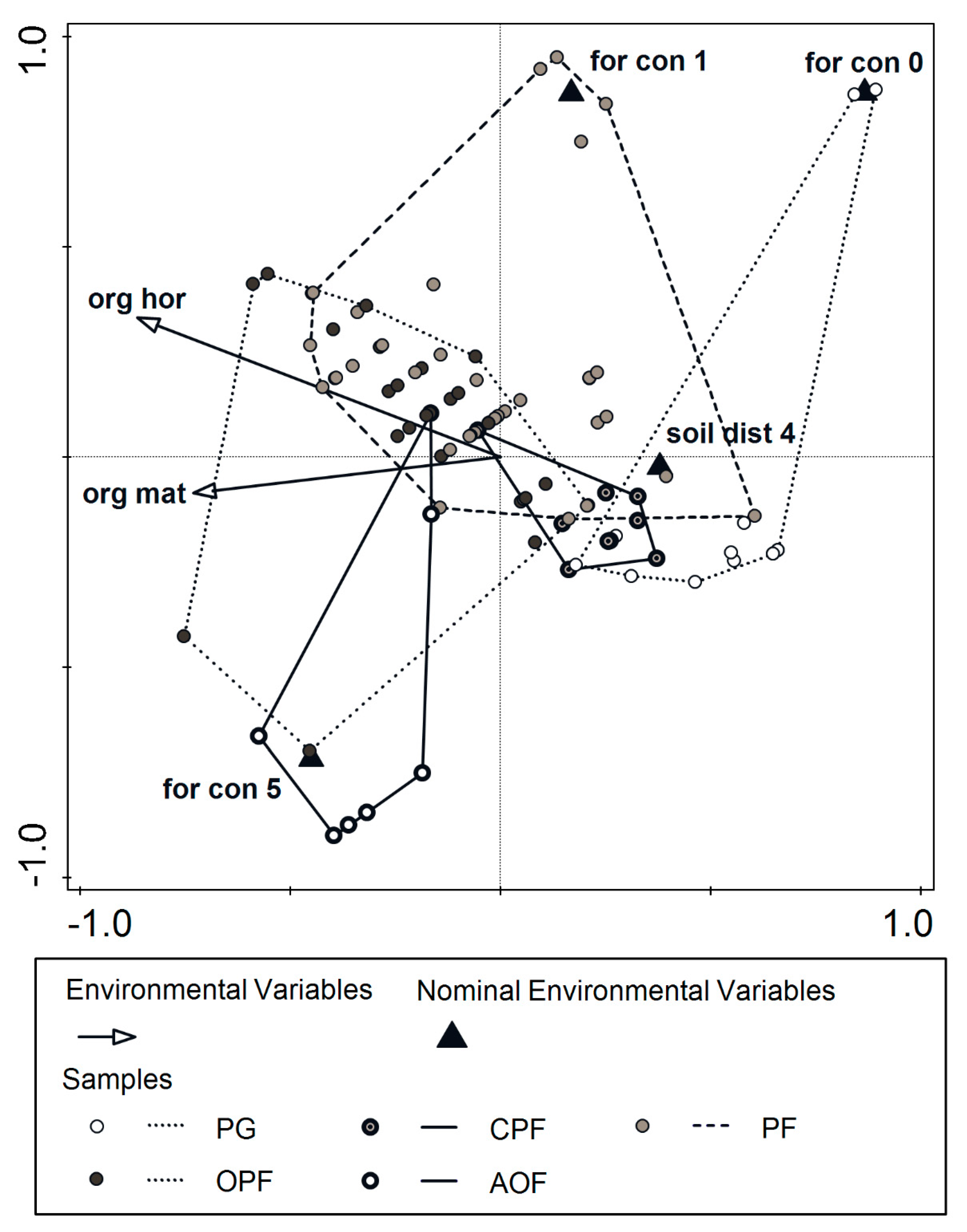
| Full Name | Short Name | Variable Type | Explains % | Contribution % | Pseudo-F | p-Value | p (Adjusted) |
|---|---|---|---|---|---|---|---|
| organic horizon thickness [mm] | org hor | general | 12.3 | 25.3 | 12.3 | 0.0001 | 0.0003 |
| forest continuity factor. for con 5 | for con 5 | factor | 8.4 | 17.2 | 9.2 | 0.0001 | 0.0003 |
| forest continuity factor. for con 0 | for con 0 | factor | 6.1 | 12.5 | 7.1 | 0.0003 | 0.0012 |
| forest continuity factor. for con 1 | for con 1 | factor | 5.9 | 12.1 | 7.4 | 0.0001 | 0.0006 |
| soil disturbance factor. soil dist 4 | soil dist 4 | factor | 2.6 | 5.4 | 3.4 | 0.0001 | 0.0005 |
| organic matter content in soil at 10 cm depth [%] | org mat | general | 1.4 | 2.8 | 1.8 | 0.0113 | 0.0387 |
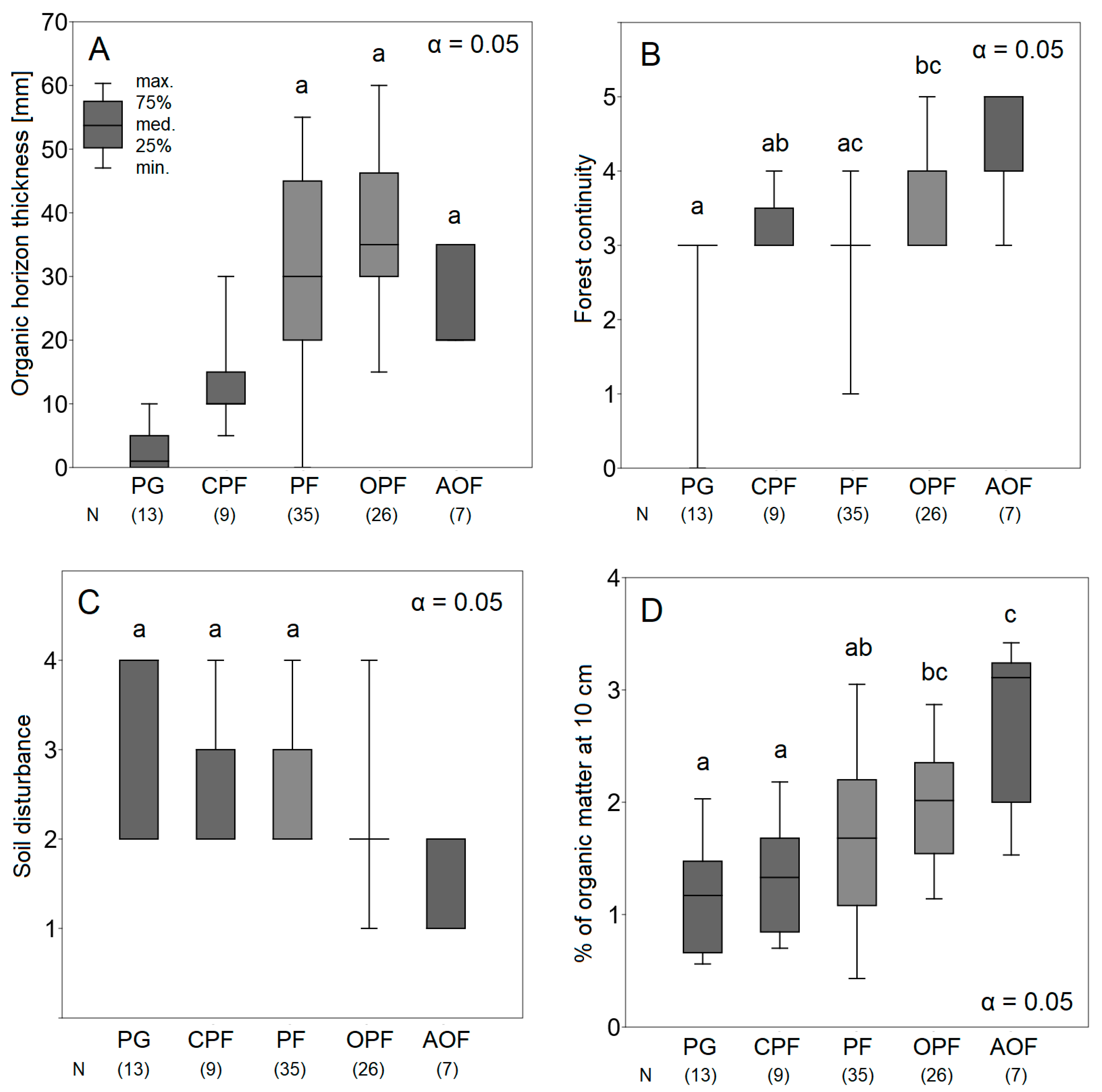
| Group of Plots | PG | CPF | PF | OPF | AOF |
|---|---|---|---|---|---|
| Number of samples | 13 | 9 | 35 | 26 | 7 |
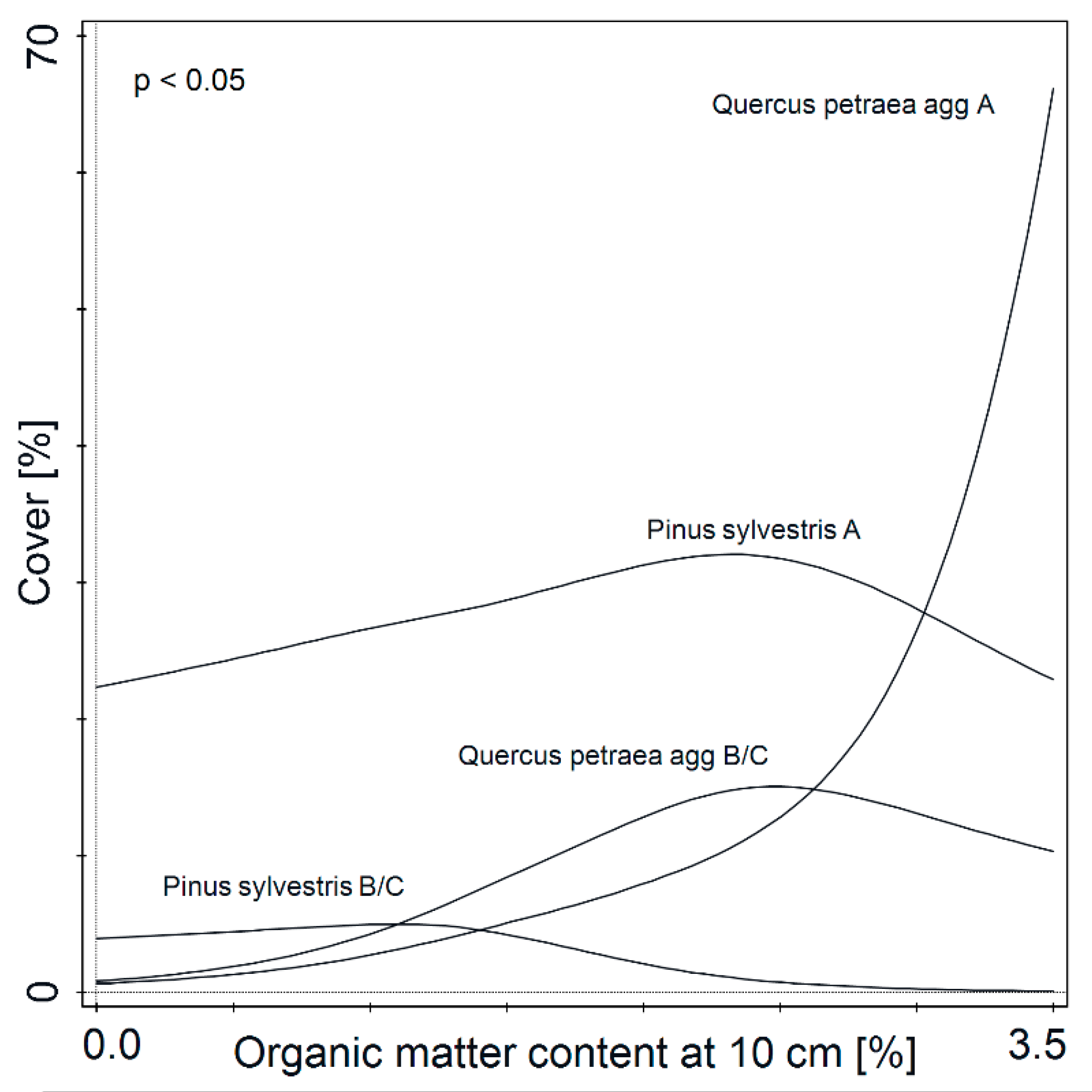
| Quercus petraea (Matt.) Liebl. agg A | 0.038 | 0.389 | 0.057 | 11.827 42.6 | 68.714 54.2 |
| Quercus petraea agg B/C | 2.481 | 1.323 | 2.603 | 26.154 | 5.214 |
| Pinus sylvestris L. A | 6.692 | 17.333 | 46.286 22.8 | 27.346 22.8 | 3.857 |
| Juniperus communis L. B/C | 2.17 | 0.578 | 0.563 | 1.413 | 0.943 |
| Betula pendula Roth A | 2.669 | 19.778 53.7 | 0.271 | 2.027 | 1.714 |
| Pinus sylvestris B/C | 14.154 26.2 | 2.157 | 1.298 | 0.783 | 0.006 |
| Convallaria majalis L. | 0 | 0 | 0 | 0.008 | 4.357 78.8 |
| Hieracium lachenalia C. C. Gmel. | 0.001 | 0 | 0.006 | 0.008 | 0.257 78 |
| Calamagrostis arundinacea (L.) Roth | 0 | 0 | 0 | 0.008 | 0.171 57.6 |
| Polytrichastrum formosum (Hedw.) GL Smith | 0 | 0.022 | 0.007 | 0.016 | 0.559 59.9 |
| Siuro-hypnum oedipodium (Mitt.) Ignatov & Huttuman | 0.246 | 0.001 | 3.167 | 0.126 | 0.174 39.6 |
| Hieracium murorum L. | 0 | 0 | 0 | 0 | 0.003 49.2 |
| Carex pilulifera L. | 0 | 0.023 | 0.017 | 0.197 14.5 | 1.457 56.8 |
| Pteridium aquilinum (L.) Kuhn | 0 | 0 | 0.006 | 0.497 12 | 3.957 61.9 |
| Vaccinium myrtillus L. | 0.015 | 0.056 | 0.661 | 4.708 16.5 | 14.571 39.1 |
| Melampyrum pretense L. | 0.247 | 0.512 | 0.712 | 1.697 21.4 | 1.373 |
| Calluna vulgaris (L.) Hull | 0 | 0.022 | 0 | 0.37 22.6 | 0.071 |
| Pleurozium schreberi (Brid.) Mitt | 2.24 | 11.212 | 55.392 17.2 | 52.731 | 7.7 |
| Hieracium pilosella L. | 2.169 | 0.412 | 0.133 | 0.021 | 0 |
| Vaccinium vitis-idaea L. | 0 | 0 | 0.001 | 0.354 | 0.001 |
| Dicranum polysetum Swartz | 3.185 | 8.8 | 8.581 | 7.008 | 0.93 |
| Dicranum scoparium Hedw. | 4.493 | 14.446 | 6.306 | 3.134 | 0.09 |
| Leucobryum glaucum (Hedw.) Ångstr. | 0 | 0.056 | 0.006 | 0 | 0.029 |
| Deschampsia flexuosa (L.) Trin | 0 | 0 | 0 | 0.008 | 0 |
| Cladonia rangiferina (L.) Weber ex F.H.Wigg. | 0 | 8.667 39.9 | 0.101 | 0.008 | 0 |
| Cladonia furcata (Huds.) Schrad. | 0.017 | 0.179 34.4 | 0.662 | 0.249 | 0 |
| Festuca ovina L. | 0.463 | 3.137 28.2 | 0.051 | 0.832 | 3.429 |
| Cladonia gracilis (L.) Willd. | 0.586 26.3 | 3.467 57.3 | 0.304 | 0.058 | 0 |
| Cladonia arbuscula ssp. mitis | 19.001 31.1 | 33.389 54.3 | 0.831 | 1.335 | 0 |
| Cladonia uncialis (L.) Weber ex F.H. Wigg. | 4.962 37.9 | 0.867 50.1 | 0.132 | 0.008 | 0 |
| Cladonia phyllophora Ehrh. ex Hoffm. | 0.956 37.6 | 0.137 34.9 | 0.108 | 0 | 0 |
| Corynephorus canescens (L.) P.Beauv. | 1.132 57.9 | 0.103 31.3 | 0.129 | 0 | 0 |
| Cephaloziella divaricata (Sm.) Schiffn. | 0.032 34.4 | 0 | 0.001 | 0 | 0 |
| Cetraria aculeata (Schreb.) Fr. | 0.941 70.5 | 0 | 0.006 | 0 | 0 |
| Cladonia cervicornis (Ach.) Flot. | 0.523 56.4 | 0 | 0.001 | 0 | 0 |
| Cladonia macilenta Hoffm. | 0.804 41.9 | 0.003 | 0.02 | 0.011 | 0 |
| Polytrichum piliferum Hedw. | 6.208 54.7 | 0.08 | 0.715 | 0 | 0 |
| Stereocaulon condensatum Hoffm. | 0.569 61.1 | 0 | 0 | 0 | 0 |
Publisher’s Note: MDPI stays neutral with regard to jurisdictional claims in published maps and institutional affiliations. |
© 2022 by the authors. Licensee MDPI, Basel, Switzerland. This article is an open access article distributed under the terms and conditions of the Creative Commons Attribution (CC BY) license (https://creativecommons.org/licenses/by/4.0/).
Share and Cite
Zaniewski, P.T.; Obidziński, A.; Ciurzycki, W.; Marciszewska, K. Past Disturbance–Present Diversity: How the Coexistence of Four Different Forest Communities within One Patch of a Homogeneous Geological Substrate Is Possible. Forests 2022, 13, 198. https://doi.org/10.3390/f13020198
Zaniewski PT, Obidziński A, Ciurzycki W, Marciszewska K. Past Disturbance–Present Diversity: How the Coexistence of Four Different Forest Communities within One Patch of a Homogeneous Geological Substrate Is Possible. Forests. 2022; 13(2):198. https://doi.org/10.3390/f13020198
Chicago/Turabian StyleZaniewski, Piotr T., Artur Obidziński, Wojciech Ciurzycki, and Katarzyna Marciszewska. 2022. "Past Disturbance–Present Diversity: How the Coexistence of Four Different Forest Communities within One Patch of a Homogeneous Geological Substrate Is Possible" Forests 13, no. 2: 198. https://doi.org/10.3390/f13020198