Abstract
Dead wood (DW) is an important component of sustainable forest management and climate change mitigation. Three research plots (each with an area of 1 ha), located in virgin forests in the Southern Carpathians (Semenic P20, Retezat–Zănoaga, and Făgăraș–Șinca), were installed in order to study the synergies between DW and climate change mitigation effects. Data on the dendrometric characteristics of standing and lying DW, the species, and the degree of decay were recorded. The aboveground biomass (AGB) and carbon stock (CS) of the DW were also determined. The DW volume was between 48 m3·ha−1 and 148 m3·ha−1, with the total volume (dead and alive) ranging between 725 m3·ha−1 and 966 m3·ha−1. The DW volume distribution shows a decreasing trend, with the most suitable theoretical distributions for describing this being the lognormal, the 2P Weibull, and the 2P-Gamma. The AGB ranged between 17 t·ha−1 and 30 t·ha−1 and showed a decreasing trend according to altitude. The CS was between 8 t·ha−1 and 14.33 t·ha−1. A slow decomposition rate for the hardwood was identified by analyzing the relationship between the surface and volume of the DW. This highlighted the capacity of DW to store carbon for a long period of time.
1. Introduction
Concerns regarding climate change are becoming more and more obvious. It is well known that forests are an important component of the global carbon cycle [1], with dead wood (DW) being a key element of sustainable forest management [2,3]. Virgin forests are reference models for managed forests [4,5,6], and the most appropriate way to understand the synergies between DW and climate change mitigation is to research this topic in natural forests [2].
Virgin forests consist of different-aged trees, which reach impressive dimensions at old age [7], their diameter distribution being, in general, ‘J’-shaped [8]. All trees reach their physiological age (longevity) and then, ultimately, they die and become DW. Dead wood can actually be considered as living wood because it maintains life in the form of different types of insects, mushrooms, and mammals, for example, by providing food and shelter [9]. In managed forests, the natural developmental stages of the trees are missing, causing the disappearance of the floras and faunas that are specific to virgin forests [10,11,12,13]. In the last few decades, in Romania, the concept of ‘close-to-nature’ forest management has been adopted because its characteristics (natural regeneration, single-tree felling, indigenous tree species, etc.) [7] promote the better management of forests. The period prior to 1990 had a relatively negative impact on the state of forest ecosystems in Romania, as well as in other Carpathian countries, where the productive functions of forests were prioritized. Subsequently, based on research findings, especially those concerning the protective functions of forests, it was recommended for the first time in 1995 that a minimum volume of DW (15–20 m3·ha−1) needed to be maintained in the forests [13]. With the evolution and development of this type of research worldwide [14,15,16,17,18,19], concerns regarding this have emerged, and the amount of DW has increased significantly. Research on establishing and monitoring the health condition [20], the causes of tree death, and the dynamics of DW has also intensified [21,22].
Forest vegetation stores significant amounts of carbon, thus helping to mitigate climate change [23]. Trees store higher amounts of carbon in their youth, due to more intense growth processes [24] compared to mature trees. The next steps are the transformation of living wood into dead wood or the transformation of wood into products.
Products resulting from the primary processing (eq: logs, lumber, laminated wood) or secondary wood (buildings, walls, frames, windows, doors, floors and ceilings, textiles, furniture, packaging, paper) store different amounts of carbon. This differentiation is related to the product category from which it is a part of [25].
The presence of DW in forests is important because it stores carbon from the atmosphere [26], which makes it relevant for estimating the carbon stock (CS). Current concerns regarding global warming have highlighted the importance of DW, aboveground biomass (AGB), and CS studies due to the fact that, in DW, a significant amount of biomass and carbon is stored [27].
As climate change is becoming more evident [28], efforts to mitigate its effects have intensified [29] and, through the actions mentioned in the Paris Agreement [30], Glasgow COP [31], there is a desire for the transition to a carbon-neutral society, part of which involves the important role of land use and land-use change in the forest sector (LULUCF) [32]. DW plays an important role in carbon and nutrient cycling [9] as well as in the National Inventory of Greenhouse Gas Emissions reporting under climate change regulations [33] because it stores carbon for a long period of time [34] and can, thus, help to reduce the effects of climate change [35]. The aim of our study was to emphasize the importance of DW in the sustainable functioning of forest ecosystems. The objectives of the research were (i) to determine the quantitative and qualitative indices of DW and their relationships with stand variables and (ii) to estimate the AGB and CS resulting from DW present in our research areas.
2. Materials and Methods
2.1. Study Location
Three research plots, each with an area of 1 ha, were installed in the Southern Carpathians (Figure 1) in a temperate continental climate, exhibiting various peculiarities of the area. The peculiarities were determined by the altitude and orientation of mountain peaks. These research areas were also characterized by a short vegetative season (maximum of 3 months) and were sometimes affected by late frosts.
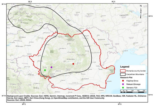
Figure 1.
Research plot location.
The research plots had never been influenced by anthropogenic activities, a fact proved by the absence of traces of timber harvest, new or old, but also by the lack of information from forest management plans. Above that, they preserved the structural characteristics of virgin forests (all plots were situated in protected areas), and they were chosen using criteria found in the literature [36,37]. Some of these criteria are uneven age, high biodiversity, no human intervention, large amounts of dead wood, no access roads, etc.
The forests in which the research plots were placed are located in different parts of the Southern Carpathians and are at different altitudes, characterized by different compositions in terms of forest species (Table 1).

Table 1.
Main characteristics of the research plots.
2.2. Sampling of DW and Living Trees
The DW (standing and lying) was sampled. The standing DW (SDW) included all trees with a diameter at breast height (dbh) higher than 8 cm (88 snags), and the lying DW (LDW) included all the samples with top diameters (thinner end) of more than 8 cm (241 samples), all measured using a caliper/tape measure at intervals of one meter. For the LDW with advanced degrees of decay, the diameters were measured using a caliper so as not to damage the sample. Data regarding the species or groups of species (coniferous, beech, and other deciduous) and the DW decay category (Table 2) were also recorded, along with data on the height of the SDW and the length of the LDW, which were measured using a Vertex IV (height) dendrometer and tape measure (dbh). For LDW sections lying partially outside the research plot boundaries, only the parts inside the plot were counted.
Table 2.
Dead wood categories depending on decay stages.
For decay classification, we used the methodology proposed in other similar research [38,39,40], presented in Table 2.
Sampling of the living trees was carried out by measuring and recording different characteristics, such as the dbh and height, with the same instruments used for the DW. Species data were also recorded.
2.3. Data Analysis
The SDW and living tree volumes were determined using Equation (1) [40].
where h represents the height of the SDW; d represents the dbh; v represents the volume of the SDW; and a0, a1, a2, a3, and a4 are regression coefficients customized for each species [40] from Romanian dendrometrics tables [41].
In some cases where the SDW had no top, the samples were photographed, and their heights and diameters at 1 m high were measured in order to allow for the application of the Huber formula (Equation (2)) [42]. Afterwards, the photographs were given a scale using AutoCAD Raster Design software, and the rest of the diameters were estimated in order to apply the Huber formula to determine the volume.
where l is the length of the DW sample and d is the diameter (in cm) of the middle of the DW samples.
To describe the DW volume distribution, the 2-parameter Lognormal [43], Weibull [44], and Gamma [45] theoretical functions were used due to their flexibility and applicability in describing uneven-aged forest distributions. The same theoretical distributions were also used to test the similarity between the stand distributions in all the plots. The goodness of fit was tested using the χ2 criterion and the Kolmogorov–Smirnov [46] and the Anderson–Darling [47] tests. The aim of identifying the most appropriate theoretical distributions of the DW volume is to adopt specific forest management in order to obtain the optimal structures of the stands. Specifically, by maintaining or extracting specific dead wood volumes, the health of forest can be maintained and more carbon can be stored.
The amounts of dry AGB, represented by the biomass of branches and trunks, and CS in the DW were determined differently, using the DW decay categories (S1, S2, L1, L2). Currently, there are several methodologies for determining the biomass and CS, but in order for our results to be comparable with other datasets, we decided to use a rapid and easy method that has already been widely used (e.g., in national inventory reporting under climate change regulations). Thus, for the SDW, the dry AGB was calculated by multiplying the volume by the wood density [48].
For the wood density, we used the values from the Romanian dendrometrics tables (beech 545 kg/m3, coniferous 335 kg/m3, and other deciduous 530 kg/m3) [41], first applying a density-reduction factor based on the degree of deterioration of the wood [49] obtained from the decay stage classification recorded in the field. The information on wood density from the Romanian dendrometrics tables are nationally determined and representative, containing data on dry wood density.
For the transformation of DW biomass into stored carbon, we used Equation (3) [48], with the dry AGB and carbon fraction (CF) as the variables. The CF value used was 0.47 t C ha−1 [50].
The dry AGB of the LDW was determined by multiplying the volume by the medium-density class [48,51]. The CS of the LDW was determined using a relation similar to the one used for the SDW, with dry AGB and CF being the variables [48].
For each dead wood sample (SDW or LDW), its projection (surface) was determined using the diameter and height (length in the case of LDW) data. SDW samples were considered as a cone, and their ground projection was calculated using the equilateral triangle area formula; LDW samples were considered a cone trunk and their ground projection was calculated using the equilateral trapezoidal area formula.
All this was necessary to compute the surface-to-volume ratio, which is the ratio between the area of the piece and its volume [52].
The statistical parameters for describing the DW volume distributions were determined using the R PASTECS package from R software [53]. This analysis was performed in order to provide a brief summary of the samples and analyzes used in the study.
3. Results
3.1. Descriptive Statistic
A high variability was observed in terms of the number of DW samples and volume, although this variability was not recorded in the mean volume, as evidenced by the coefficient of variation (Table 3).
Table 3.
Descriptive statistics of dead wood volume distributions.
The total volume of DW recorded was quite high, varying between 48 m3·ha−1 (Semenic P20 plot) and 148 m3·ha−1 (Făgăraș–Șinca plot). In each plot, the DW sample volume showed a very high diversity, specific to this type of forests (virgin forests), as indicated by the coefficient of variation values. This situation can be explained by very intense inter- and intra-competition processes and also by the presence of a very high number of senescence trees.
3.2. Dead Wood Distribution according to the Category of Decay and Its Volume according to Species and Living Trees
In all the research plots, most of the DW fell into the log 2 category (soft LDW without bark) (Figure 2).
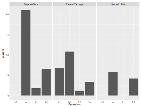
Figure 2.
Dead wood distribution in relation to decay class.
The volume of DW from coniferous trees was higher than the volume from beech or other deciduous species in the Retezat–Zănoaga (Figure 3) and Făgăraș–Șinca plots, reaching a value of 114 m3·ha−1. The largest quantity of beech DW was found in Semenic P20, followed by Făgăraș–Șinca and Retezat–Zănoaga. This is normal, taking into account that in Semenic P20, the majority species is beech The values recorded in the other plots (where beech is not the main species) were higher compared to those recorded in managed forests [35]. The presence of other deciduous samples was reduced, being closely related to the amount of living trees of those species.
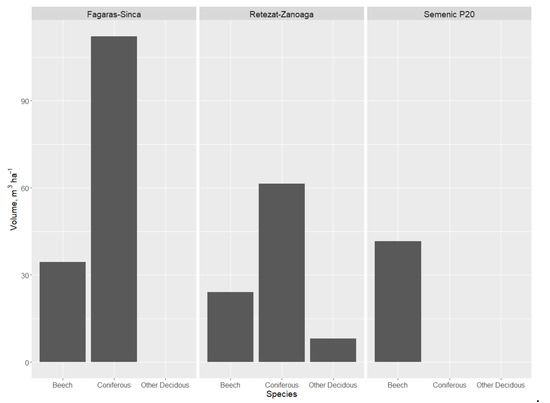
Figure 3.
Dead wood volume in relation to species group.
Of the total research plot volume (living and dead wood), the volume of coniferous DW varied between 16% in Retezat–Zănoaga and 25% in Făgăraș–Șinca. For beech, the DW percentage of the total research plot volume was lowest in Retezat–Zănoaga—a mixed forest—and highest in Semenic P20—a pure beech forest (Table 4). For the other deciduous trees (sycamore and mountain elm), the volume was 8 m3·ha−1 (Retezat–Zănoaga). The total DW volume ranged between 48 m3·ha−1 (in Semenic P20) and 148 m3·ha−1 (in Făgăraș–Șinca), with the total volume (dead and alive) ranging between 725 m3·ha−1 and 964 m3·ha−1.
Table 4.
Volume of dead wood and living trees related to the group of species.
3.3. Fitting of Experimental Dead Wood (DW) Volume Distribution
The DW volume experimental distribution (recorded from field data) showed a decreasing trend (Figure 4), with high values for the small categories and a reversed ‘J’ shape, indicating that smaller trees were more vulnerable to natural selection generated by inter- and intra-specific competition and forest development stage.
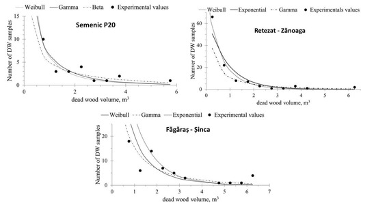
Figure 4.
Fitting of experimental DW volume distribution.
The results of the goodness-of-fit tests indicate that, for the Semenic P20 plot, all the studied distribution laws were suitable for describing the distribution of the DW volume (Table 5). The experimental distributions of DW volume in the Retezat–Zănoaga and Făgăraș–Șinca plots, when compared to the lognormal and 2P Weibull theoretical laws, did not show any differences, according to the Kolmogorov–Smirnov and Anderson–Darling conformity tests.
Table 5.
Experimental values of volume of dead wood specific goodness of fit tests.
3.4. Estimating the above Ground Biomass and Carbon Stock. Quantity of AGB and CS of DW in Relation to Altitude
For our research area, the quantities of AGB and CS show decreasing trends in relation to altitude (Table 6), ranging from 17.4 t·ha−1 (Semenic P20) to 30.51 t·ha−1 (Retezat–Zănoaga). In terms of the CS, the values vary between 8.17 t·ha−1 (Semenic P20) and 14.33 t·ha−1 (Retezat–Zănoaga), with an average of 11.58 t·ha−1.
Table 6.
Quantity of AGB and CS in relation with altitude.
With the exception of the Semenic P20 plot, the greatest amounts of AGB and CS were recorded in the LDW category.
3.5. The Relation between Surface and Volume of DW and Surface-to-Volume (SV) Ratio Related to the Decay Class of DW
For all the research plots, an ascending trend of the DW surface-to-volume ratio was recorded. The results indicate that the surface area of the DW was directly proportional to its volume (Figure 5). The curve describing this relationship indicates that the lowest values were recorded in the Semenic P20 plot, where the lowest volume of DW was recorded (48.9 m3·ha−1).
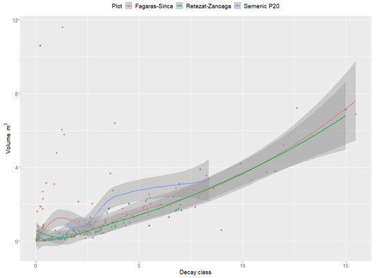
Figure 5.
Relationship between DW surface and volume.
The SV ratio index registered high values in the LDW decay class (category L2) (Figure 6). The recorded values are high for all the plots with category L1, indicating the highest values of this index was found for the Retezat–Zanoaga plot. In terms of the SDW, high values were only found in the Semenic P20 plot. The value of this indicator was very low in the other plots.
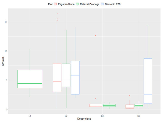
Figure 6.
Relation between surface-to-volume ratio and decay class of DW.
4. Discussion
Descriptive Statistics
The DW volume falls into the average range encountered in virgin and quasi-virgin forests (between 50 m3·ha−1 and 200 m3·ha−1) [19,54].
The DW distribution on the decay categories is similar to those found in other studies [19], indicating that the forest stands in our research plots were not influenced by anthropogenic activities, and humans did not harvest DW. The presence of DW in significant quantities is important because it stabilizes the ecosystem, in part by protecting the soil against erosion, contributing to the soil quality via massive organic and mineral inputs, and improving soil water retention [55,56,57]. In addition, it provides food and habitats for many species (plants, animals, and fungi), as well as maintaining ecosystem health [2,21,27,58].
The proportion of DW in terms of species was similar to what has been reported in the literature [59], with the amount of DW from deciduous trees being less than that of conifers. This can be explained by coniferous trees being more vulnerable to accidental natural disturbances, such as windthrow [60] and snow breaks. In addition, in our research plots, the physiological ages (longevity age) of the coniferous trees were lower than the physiological ages of the beech trees, which implies that the amount of DW would be higher in coniferous trees [61].
The relationship between DW and living tree volumes has been highlighted previously [27,62], and recent studies performed in virgin forests in the Semenic Mountains (Southern Carpathians) have shown that the volume of dead wood there varied between 50 m3·ha−1 and 223 m3·ha−1 [21].
The percentage of DW in relation to the total volume (dead and alive) was similar to other areas [59], with the proportion of living wood volume to DW volume also being similar—around 76% of the total volume is represented by the living tree volume [63,64,65]. These percentages are closely related to the composition of the species and their physiology, as mentioned above.
By fitting the experimental DW volume distribution, we can observe a decreasing trend similar to the ones shown in previous studies [19]. The distribution is characterized by the presence of DW in the small volume category, as a result of intraspecific competition [66]. In addition, this highlights that in virgin forests, nature, without human intervention, naturally tends the stands [7].
In addition, the fact that this distribution follows the laws of known theoretical distributions is helpful in terms of being able to reproduce them through forest management in order to achieve a sustainable and efficient management regime [6].
Regarding the quantity of AGB and CS determined in our study, similar results have been obtained in the Rocky Mountains (USA), where anthropogenic influences are low, and the quantity of AGB varies between 4.75 t·ha−1 and 53.97 t·ha−1 [27], suggesting that our results can be compared with those from other studies, and that they could be considered a legitimate DW data source.
The recorded values of AGB and CS indicate that forests, especially virgin forests, have a very important role in the carbon storage cycle, which is a significant contribution to mitigating global warming effects. The outcomes of recent studies have revealed that global warming leads to enhanced DW decomposition and, implicitly, to the loss of stored carbon [27]. Therefore, maintaining these multifunctional ecosystems in an intact state should be viewed as vitally important. The recorded CS value was below the ‘normal’ average (17 t·ha−1), as found in another study [67]. In terms of the capacity for greater carbon storage to induce higher biodiversity potential [68], it has been proven that lower amounts of DW are sufficient for maximum biodiversity in warm regions, but higher amounts are needed in cool climates [69]. Despite the fact that wood products store carbon for a longer period of time, it is necessary to maintain a minimum amount of DW. This minimum is necessary to maintain an optimal level of biodiversity.
Studies on the AGB and CS in relation to other variables, such as altitude, are crucial for understanding the importance of virgin forests in slowing global warming. Our research, along with other studies [27,62,70], highlights that the DW biomass decreases with altitude and, implicitly, with air temperature [69].
The SV ratio is very important because it can indicate the presence of different organisms, such as arthropods [71,72,73], if high values are recorded [52]. This is applicable to the L2 (all research plots) and L1 (the Retezat–Zanoaga plot) decay categories. These values also indicate a slow hardwood decomposition rate [52,72,73,74] in larger trees, which could affect the DW breakdown rates [75]. Recent studies have shown that DW decomposes through natural processes over approximately 40–50 years [70]. This aspect is very important because carbon is stored in the DW for a long period of time, producing an additional impact on climate change mitigation.
In terms of the SV ratio and DW decay classes, the lack of DW in the small log category indicates that the DW was decomposed faster by arthropods, as supported by the high ratios [52] and confirmed in Semenic P20 by the presence of low volumes of LDW, assuming that the loss of LDW increased the SV ratio. The presence of significant quantities of DW, with the highest degree of decomposition and high porosity over large areas, indicates that the DW has a high water storage capacity and absorbability. Additionally, the amount of water supplied to the forest can be influenced by regulating the quantity and species composition of DW [76]. If this assumption is proven true in future studies, this information may be useful in forest management [77,78]. The explanation is that the water retained in these ecosystems could have a special significance in terms of water quality, hydrology, and, last but not least, climate regulation [27,79].
In forest ecosystems, the major processes, such as birth, interaction, growth, and death, are always closely connected, and the hypothesis that plant life is directly dependent on interaction and growth is obvious [80].
Starting from the idea that it is well known that forest productivity is influenced by structural characteristics and biodiversity indicators [24,81,82,83], and because DW is an indicator of biodiversity, we notice that the importance of DW is relatively large, even at a global level [83].
5. Conclusions
Based on the findings of this study, we have reached the following main conclusions:
In analyzing the DW volume data, it was found that the results were very homogeneous and similar to those of other virgin and quasi-virgin forests (50 m3·ha−1 and 200 m3·ha−1, respectively). The plots had not been influenced by human activities because the DW decay distribution showed a high quantity of DW from the category of soft LDW without bark. The vulnerability of coniferous trees to accidental natural factors (snow break, windthrow) in comparison to beech and other broadleaved trees was highlighted. Another reason for the presence of higher amounts of coniferous DW is that this group of species has a lower longevity compared to other species in the plots.
In order to achieve sustainable and efficient forest management in the future, we identified a potential tool that could reproduce the structure of the DW volume in managed forests. This tool uses theoretical distributions, such as Lognormal, 2P Weibull, and Gamma, because, in this study, these were suitable for describing the DW volume distribution.
The quantities of AGB and CS recorded were very consistent (between 17.4 t·ha−1 and 30.51 t·ha−1), decreasing with altitude. In addition, DW has an important role in enhancing biodiversity, carbon sequestration, and therefore, mitigating climate change. From analyzing the surface area and volume of DW, our findings indicate that hardwood has a slow decomposition rate.
Accordingly, carbon is stored in DW for a long period of time, which contributes to climate change mitigation. In addition, significant quantities of DW with a high degree of decomposition have a large water storage capacity, adsorbing water in forests and thereby playing a very important role in climate regulation.
Recently, the interest in DW is increasing as its benefits for climate change mitigation become better understood. Therefore, it is recommended that a minimum quantity of DW be left in managed forests in order to help reduce the effects of climate change.
Author Contributions
Conceptualization, Ș.C. and O.B.; methodology, Ș.C. and D.P.; software, Ș.C.; validation, Ș.C., B.A., and O.B.; formal analysis, Ș.C.; investigation, Ș.C.; resources, Ș.C. and O.B.; data curation, Ș.C.; writing—original draft preparation, Ș.C. and D.P.; writing—review and editing, Ș.C., D.P., B.A., Ș.L., and O.B.; visualization, Ș.C. and Ș.L.; supervision, Ș.C. and O.B.; project administration, Ș.C. and O.B.; funding acquisition, Ș.C. and O.B. All authors have read and agreed to the published version of the manuscript.
Funding
This research was funded partially by Romanian Ministry of Research, Innovation and Digitization and Innovation, within the Nucleu BIOSERV National Programme (Contract No. 12N/2019), Project IDs PN 19070101 and PN 19070103, and partially by the CresPerfInd project—“Creșterea capacității și performanței instituționale a INCDS, Marin Drăcea” în activitatea de CDI—CresPerfInst (Contract No. 34PFE./30.12.2021) financed by the Ministry of Research, Innovation and Digitization through Program 1—Development of the national research—development system, Subprogram 1.2—Institutional performance—Projects to finance excellence in RDI.
Conflicts of Interest
The authors declare no conflict of interest.
References
- Hararuk, O.; Kurz, W.A.; Didion, M. Dynamics of Dead Wood Decay in Swiss Forests. For. Ecosyst. 2020, 7, 36. [Google Scholar] [CrossRef]
- Lo Monaco, A.; Luziatelli, G.; Latterini, F.; Tavankar, F.; Picchio, R. Structure and Dynamics of Deadwood in Pine and Oak Stands and Their Role in CO2 Sequestration in Lowland Forests of Central Italy. Forests 2020, 11, 253. [Google Scholar] [CrossRef]
- Bujoczek, L.; Bujoczek, M.; Zięba, S. How Much, Why and Where? Deadwood in Forest Ecosystems: The Case of Poland. Ecol. Indic. 2021, 121, 107027. [Google Scholar] [CrossRef]
- Parviainen, J. Virgin and Natural Forests in the Temperate Zone of Europe. For. Snow Landsc. Res. 2005, 79, 10. [Google Scholar]
- Vacek, S.; Vacek, Z.; Podrázskỳ, V.; Bílek, L.; Bulušek, D.; Štefančík, I.; Remeš, J.; Štícha, V.; Ambrož, R. Structural Diversity of Autochthonous Beech Forests in Broumovské Stěny National Nature Reserve, Czech Republic Strukturelle Diversität von Autochthonen Buchenwäldern Im Nationalen Naturschutzgebiet Broumovské Stěny, Tschechische Republik. Austrian J. For. Sci. 2014, 4, 191. [Google Scholar]
- Chivulescu, S.; Ciceu, A.; Leca, S.; Apostol, B.; Popescu, O.; Badea, O. Development Phases and Structural Characteristics of the Penteleu-Viforta Virgin Forest in the Curvature Carpathians. iForest 2020, 13, 389–395. [Google Scholar] [CrossRef]
- Matović, B.; Koprivica, M.; Kisin, B.; Stojanović, D.; Kneginjić, I.; Stjepanović, S. Comparison of Stand Structure in Managed and Virgin European Beech Forests in Serbia. Šumarski List 2018, 142, 47–57. [Google Scholar] [CrossRef]
- Westphal, C.; Tremer, N.; von Oheimb, G.; Hansen, J.; von Gadow, K.; Härdtle, W. Is the Reverse J-Shaped Diameter Distribution Universally Applicable in European Virgin Beech Forests? For. Ecol. Manag. 2006, 223, 75–83. [Google Scholar] [CrossRef]
- Burton, J.E.; Bennett, L.T.; Kasel, S.; Nitschke, C.R.; Tanase, M.A.; Fairman, T.A.; Parker, L.; Fedrigo, M.; Aponte, C. Fire, Drought and Productivity as Drivers of Dead Wood Biomass in Eucalypt Forests of South-Eastern Australia. For. Ecol. Manag. 2021, 482, 118859. [Google Scholar] [CrossRef]
- Bücking, W. Naturwaldreservate:” Urwald” in Deutschland; AID: Bonn, Deutschland, 2003. [Google Scholar]
- André, J. Activité et Diversité Des Organismes Hétérotrophes: Les Clés Du Bouclage Des Cycles Biogéochimiques et Sylvigénétiques. Bois Mort et à Cavité-une Clé pour les Vivantes; Lavoisier: Paris, France, 2005; pp. 89–98. [Google Scholar]
- Radu, S.; Coanda, C. Lemnul Mort și Rolul Acestora în Ecositemele Forestiere Virgine și Cvasivirgine. In Pădurile Virgine și Cvasivirgine ale Romaniei; Editura Academiei Române: Bucharest, Romania, 2013. [Google Scholar]
- Giurgiu, V. Protejarea si Dezvoltarea Durabila a Padurilor României; Editura Arta Grafica: Bucuresti, Romania, 1995; p. 400. [Google Scholar]
- Jonsell, M.; Nittérus, K.; Stighäll, K. Saproxylic Beetles in Natural and Man-Made Deciduous High Stumps Retained for Conservation. Biol. Conserv. 2004, 118, 163–173. [Google Scholar] [CrossRef]
- Ranius, T.; Ekvall, H.; Jonsson, M.; Bostedt, G. Cost-Efficiency of Measures to Increase the Amount of Coarse Woody Debris in Managed Norway Spruce Forests. For. Ecol. Manag. 2005, 206, 119–133. [Google Scholar] [CrossRef]
- Abrahamsson, M.; Lindbladh, M. A Comparison of Saproxylic Beetle Occurrence between Man-Made High-and Low-Stumps of Spruce (Picea Abies). For. Ecol. Manag. 2006, 226, 230–237. [Google Scholar] [CrossRef]
- Keeton, W.S. Managing for Late-Successional/Old-Growth Characteristics in Northern Hardwood-Conifer Forests. For. Ecol. Manag. 2006, 235, 129–142. [Google Scholar] [CrossRef]
- Bauhus, J.; Puettmann, K.; Messier, C. Silviculture for Old-Growth Attributes. For. Ecol. Manag. 2009, 258, 525–537. [Google Scholar] [CrossRef]
- Seidling, W.; Travaglini, D.; Meyer, P.; Waldner, P.; Fischer, R.; Granke, O.; Chirici, G.; Corona, P. Dead Wood and Stand Structure—Relationships for Forest Plots across Europe. iForest 2014, 7, 269–281. [Google Scholar] [CrossRef]
- Barmpoutis, P.; Stathaki, T.; Kamperidou, V. Monitoring of Trees’ Health Condition Using a Uav Equipped with Low-Cost Digital Camera. In Proceedings of the ICASSP 2019—2019 IEEE International Conference on Acoustics, Speech and Signal Processing (ICASSP), Brighton, UK, 12–17 May 2019; pp. 8291–8295. [Google Scholar]
- Tomescu, R.; Târziu, D.R.; Turcu, D.O. The Importance of Dead Wood in the Forest. ProEnvironment Promediu 2011, 4, 10–19. [Google Scholar]
- Chivulescu, Ș.; Leca, Ș.; Silaghi, D.; Cristea, V. Structural biodiversity and dead wood in virgin forests from eastern carpathians. Agric. For. 2018, 64, 177–188. [Google Scholar] [CrossRef]
- Węgiel, A.; Polowy, K. Aboveground Carbon Content and Storage in Mature Scots Pine Stands of Different Densities. Forests 2020, 11, 240. [Google Scholar] [CrossRef]
- Barrufol, M.; Schmid, B.; Bruelheide, H.; Chi, X.; Hector, A.; Ma, K.; Michalski, S.; Tang, Z.; Niklaus, P.A. Biodiversity Promotes Tree Growth during Succession in Subtropical Forest. PLoS ONE 2013, 8, e81246. [Google Scholar] [CrossRef]
- Leskinen, P.; Cardellini, G.; González-García, S.; Hurmekoski, E.; Sathre, R.; Seppälä, J.; Smyth, C.; Stern, T.; Verkerk, P.J. Substitution Effects of Wood-Based Products in Climate Change Mitigation. Eur. For. Inst. 2018, 7, 28. [Google Scholar]
- Weggler, K.; Dobbertin, M.; Jüngling, E.; Kaufmann, E.; Thürig, E. Dead Wood Volume to Dead Wood Carbon: The Issue of Conversion Factors. Eur. J. For. Res. 2012, 131, 1423–1438. [Google Scholar] [CrossRef]
- Kueppers, L.M.; Southon, J.; Baer, P.; Harte, J. Dead Wood Biomass and Turnover Time, Measured by Radiocarbon, along a Subalpine Elevation Gradient. Oecologia 2004, 141, 641–651. [Google Scholar] [CrossRef] [PubMed]
- Hansen, J.; Fung, I.; Lacis, A.; Rind, D.; Lebedeff, S.; Ruedy, R.; Russell, G.; Stone, P. Global Climate Changes as Forecast by Goddard Institute for Space Studies Three-Dimensional Model. J. Geophys. Res. 1988, 93, 9341. [Google Scholar] [CrossRef]
- García-Oliva, F.; Masera, O.R. Assessment and Measurement Issues Related to Soil Carbon Sequestration in Land-Use, Land-Use Change, and Forestry (LULUCF) Projects under the Kyoto Protocol. Clim. Chang. 2004, 65, 347–364. [Google Scholar] [CrossRef]
- Savaresi, A. The Paris Agreement: A New Beginning? J. Energy Nat. Resour. Law 2016, 34, 16–26. [Google Scholar] [CrossRef]
- Reddy, Y.M.; Rajeev, R. Developing Glasgow Accord for COP-26 Using Game Theory. J. Clim. Chang. 2021, 7, 1–8. [Google Scholar]
- Romppanen, S. The LULUCF Regulation: The New Role of Land and Forests in the EU Climate and Policy Framework. J. Energy Nat. Resour. Law 2020, 38, 261–287. [Google Scholar] [CrossRef]
- Teran, T.; Lamon, L.; Marcomini, A. Climate Change Effects on POPs’ Environmental Behaviour: A Scientific Perspective for Future Regulatory Actions. Atmos. Pollut. Res. 2012, 3, 466–476. [Google Scholar] [CrossRef]
- Schlamadinger, B.; Bird, N.; Johns, T.; Brown, S.; Canadell, J.; Ciccarese, L.; Dutschke, M.; Fiedler, J.; Fischlin, A.; Fearnside, P.; et al. A Synopsis of Land Use, Land-Use Change and Forestry (LULUCF) under the Kyoto Protocol and Marrakech Accords. Environ. Sci. Policy 2007, 10, 271–282. [Google Scholar] [CrossRef]
- Paletto, A.; Ferretti, F.; De Meo, I.; Cantiani, P.; Focacci, M. Ecological and Environmental Role of Deadwood in Managed and Unmanaged Forests. Sustain. For. Manag.–Curr. Res. 2012, 219–238. [Google Scholar] [CrossRef]
- Korpel, Š. Obnova lesnych porastov v rubáňovom sposobe hospodárenia.[W:] Pesteni les\uu.(red. M. Vyskot M.) [Restoration of forest stands in the ruby way of management]. SZN Praha. 1978, pp. 216–359. Available online: http://www.forestportal.sk/les-pre-verejnost/o-lesoch-pre-verejnost/sprievodca-lesnickymi-vyrazmi/Stranky/obnova-lesnych-porastov.aspx (accessed on 4 February 2022).
- Leibundgut, H. Europäische Urwälder der Bergstufe: Dargestellt für Forstleute, Naturwissenschafter und Freunde des Waldes [European Primeval Forests of the Bergstufe: Represented for Foresters, Naturalists and Friends of the Forest]; Haupt: Bern, Switzerland, 1982. [Google Scholar]
- McComb, W.; Lindenmayer, D. Dying, Dead, and down Trees. In Maintaining Biodiversity in Forest Ecosystems; Hunter, M.L., Ed.; Cambridge University Press: Cambridge, UK, 1999; pp. 335–372. ISBN 978-0-521-63104-4. [Google Scholar]
- Fridman, J.; Walheim, M. Amount, Structure, and Dynamics of Dead Wood on Managed Forestland in Sweden. For. Ecol. Manag. 2000, 131, 23–36. [Google Scholar] [CrossRef]
- Atici, E.; Colak, A.; Rotherham, I. Coarse Dead Wood Volume of Managed Oriental Beech (Fagus Orientalis Lipsky) Stands in Turkey. Investig. Agrar. Sist. Recur. For. 2008, 17, 216–227. [Google Scholar] [CrossRef]
- Giurgiu, V.; Decei, I.; Drăghiciu, D. Metode şi Tabele Metode şi Tabele Dendrometrice [Methods and Yield Tables]; Editura Ceres: Bucureşti, Romania, 2004; p. 575. [Google Scholar]
- Giurgiu, V. Dendrometrie Și Auxologie Forestieră; Ceres: Bucuresti, Romania, 1979. [Google Scholar]
- Corlett, W. The Lognormal Distribution, with Special Reference to Its Uses in Economics; Cambridge University Press: Cambridge, UK, 1957. [Google Scholar]
- Sharif, M.N.; Islam, M.N. The Weibull Distribution as a General Model for Forecasting Technological Change. Technol. Forecast. Soc. Change 1980, 18, 247–256. [Google Scholar] [CrossRef]
- Hogg, R.; Craig, A. Introduction to Mathematical Statistics; Macmillan Publishing Company: New York, NY, USA, 1978. [Google Scholar]
- Stephens, M.A. Tests of Fit for the Logistic Distribution Based on the Empirical Distribution Function. Biometrika 1979, 66, 591–595. [Google Scholar] [CrossRef]
- Anderson, T.W.; Darling, D.A. A Test of Goodness of Fit. J. Am. Stat. Assoc. 1954, 49, 765–769. [Google Scholar] [CrossRef]
- Goslee, K.; Walker, S.M.; Grais, A.; Murray, L.; Casarim, F.; Brown, S. Module C-CS: Calculations for Estimating Carbon Stocks. In Leaf Technical Guidance Series for the Development of a Forest Carbon Monitoring System for REDD+; Winrock International: Little Rock, AR, USA, 2016. [Google Scholar]
- UNFCC. Estimation of Carbon Stocks and Change in Carbon Stocks in Dead Wood and Litter in A/R CDM Project Activities. 2013. Available online: https://cdm.unfccc.int/methodologies/ARmethodologies/tools/ar-am-tool-12-v3.0.pdf (accessed on 4 February 2022).
- IPCC. IPCC Guidelines for National Greenhouse Gas. Inventories; IPCC: Geneva, Switzerland, 2006; Volume 4. [Google Scholar]
- Goslee, K.; Walker, S.M.; Grais, A.; Murray, L.; Brown, S.; Goslee, K.; Walker, S.M.; Grais, A.; Murray, L.; Casarim, F.; et al. Standard Operating Procedures for Terrestrial Carbon Measurement: Version 2012; Winrock International: Little Rock, AR, USA, 2012. [Google Scholar]
- Holeksa, J. Coarse Woody Debris in a Carpathian Subalpine Spruce Forest. Forstw. Cbl. 2001, 120, 256–270. [Google Scholar] [CrossRef]
- Grosjean, P.; Ibanez, F. Package for Analysis of Space-Time Ecological Series. PASTECS. R Package; Version 1.2-0 for R v. 2.0. 0 & Version 1.0-1 for S+ 2000 rel. 2004. Available online: https://cran.r-project.org/web/packages/pastecs/index.html (accessed on 4 February 2022).
- Scherzinger, W. Naturschutz Im Wald: Qualitätsziele Einer Dynamischen Waldentwicklung; 36 Tabellen; Ulmer: Stuttgart, Germany, 1996. [Google Scholar]
- Mueller, U.G.; Gerardo, N.M.; Aanen, D.K.; Six, D.L.; Schultz, T.R. The Evolution of Agriculture in Insects. Annu. Rev. Ecol. Evol. Syst. 2005, 36, 563–595. [Google Scholar] [CrossRef]
- Stokland, J.N.; Siitonen, J.; Jonsson, B.G. Biodiversity in Dead Wood; Cambridge University Press: Cambridge, UK, 2012. [Google Scholar]
- Moose, R.A.; Schigel, D.; Kirby, L.J.; Shumskaya, M. Dead Wood Fungi in North America: An Insight into Research and Conservation Potential. Nat. Conserv. 2019, 32, 1–17. [Google Scholar] [CrossRef]
- Hodge, S.J.; Peterken, G.F. Deadwood in British Forests: Priorities and a Strategy. Forestry 1998, 71, 99–112. [Google Scholar] [CrossRef]
- Višnjić, Ć.; Solaković, S.; Mekić, F.; Balić, B.; Vojniković, S.; Dautbašić, M.; Gurda, S.; Ioras, F.; Ratnasingam, J.; Abrudan, I.V. Comparison of Structure, Regeneration and Dead Wood in Virgin Forest Remnant and Managed Forest on Grmeč Mountain in Western Bosnia. Plant. Biosyst. 2013. [Google Scholar] [CrossRef]
- Bourque, C.P.-A.; Bayat, M.; Zhang, C. An Assessment of Height–Diameter Growth Variation in an Unmanaged Fagus Orientalis-Dominated Forest. Eur. J. Forest. Res. 2019, 138, 607–621. [Google Scholar] [CrossRef]
- Petritan, I.C.; Commarmot, B.; Hobi, M.L.; Petritan, A.M.; Bigler, C.; Abrudan, I.V.; Rigling, A. Structural Patterns of Beech and Silver Fir Suggest Stability and Resilience of the Virgin Forest Sinca in the Southern Carpathians, Romania. For. Ecol. Manag. 2015, 356, 184–195. [Google Scholar] [CrossRef]
- Dimitrova, V. Zalihe Biomase Mrtvog Drva u Šumskim Ekosustavima Bukve (Fagus Sylvatica L.) Na Području Zapadnog Balkana, Bugarska. Šumar. List. 2018, 142, 363–370. [Google Scholar] [CrossRef]
- Christensen, M.; Hahn, K.; Mountford, E.P.; Odor, P.; Standovár, T.; Rozenbergar, D.; Diaci, J.; Wijdeven, S.; Meyer, P.; Winter, S.; et al. Dead Wood in European Beech (Fagus Sylvatica) Forest Reserves. For. Ecol. Manag. 2005, 210, 267–282. [Google Scholar] [CrossRef]
- Janik, D.; Adam, D.; Vrska, T.; Hort, L.; Unar, P.; Kral, K.; Samonil, P.; Horal, D. Tree Layer Dynamics of the Cahnov–Soutok near-Natural Floodplain Forest after 33 Years (1973–2006). Eur. J. For. Res. 2008, 127, 337–345. [Google Scholar] [CrossRef]
- Vrška, T.; Šamonil, P.; Unar, P.; Hort, L.; Adam, D.; Král, K.; Janík, D. Developmental Dynamics of Virgin Forest Reserves in the Czech Republic III—Šumava Mts. and Českỳ Les Mts. Diana, Stozec, Boubın Virgin Forests, Milešice Virgin Forest; Academia Prague: Praha, Czech Republic, 2012. [Google Scholar]
- Moroni, M.T. Disturbance History Affects Dead Wood Abundance in Newfoundland Boreal Forests. Can. J. For. Res. 2006, 36, 3194–3208. [Google Scholar] [CrossRef]
- Krankina, O.N.; Harmon, M. Dynamics of the Dead Wood Carbon Pool in Northwestern Russian Boreal Forests. Water Air Soil Pollut. 1995, 82, 227–238. [Google Scholar] [CrossRef]
- Ali, A.; Lin, S.-L.; He, J.-K.; Kong, F.-M.; Yu, J.-H.; Jiang, H.-S. Climate and Soils Determine Aboveground Biomass Indirectly via Species Diversity and Stand Structural Complexity in Tropical Forests. For. Ecol. Manag. 2019, 432, 823–831. [Google Scholar] [CrossRef]
- Müller, J.; Brustel, H.; Brin, A.; Bussler, H.; Bouget, C.; Obermaier, E.; Heidinger, I.M.M.; Lachat, T.; Förster, B.; Horak, J.; et al. Increasing Temperature May Compensate for Lower Amounts of Dead Wood in Driving Richness of Saproxylic Beetles. Ecography 2015, 38, 499–509. [Google Scholar] [CrossRef]
- Vlad, R.; Sidor, C.G.; Dinca, L.; Constandache, C.; Ispravnic, A.; Pei, G. Dead Wood Diversity in a Norway Spruce Forest from the Caãlimani National Park (the Eastern Carpathians). Balt. For. 2019, 25, 11. [Google Scholar] [CrossRef]
- Graham, R.L.; Cromack, K., Jr. Mass, Nutrient Content, and Decay Rate of Dead Boles in Rain Forests of Olympic National Park. Can. J. For. Res. 1982, 12, 511–521. [Google Scholar] [CrossRef]
- Harmon, M.E.; Franklin, J.F.; Swanson, F.J.; Sollins, P.; Gregory, S.; Lattin, J.; Anderson, N.; Cline, S.; Aumen, N.; Sedell, J.; et al. Ecology of Coarse Woody Debris in Temperate Ecosystems. Adv. Ecol. Res. 1986, 15, 133–302. [Google Scholar]
- Harmon, M.E.; Cromack, K., Jr.; Smith, B.G. Coarse Woody Debris in Mixed-Conifer Forests, Sequoia National Park, California. Can. J. For. Res. 1987, 17, 1265–1272. [Google Scholar] [CrossRef]
- Hérault, B.; Beauchêne, J.; Muller, F.; Wagner, F.; Baraloto, C.; Blanc, L.; Martin, J.-M. Modeling Decay Rates of Dead Wood in a Neotropical Forest. Oecologia 2010, 164, 243–251. [Google Scholar] [CrossRef]
- Elosegi, A.; Díez, J.; Pozo, J. Contribution of Dead Wood to the Carbon Flux in Forested Streams. Earth Surf. Process. Landforms 2007, 32, 1219–1228. [Google Scholar] [CrossRef]
- Klamerus-Iwan, A.; Lasota, J.; Błońska, E. Interspecific Variability of Water Storage Capacity and Absorbability of Deadwood. Forests 2020, 11, 575. [Google Scholar] [CrossRef]
- Floren, A.; Müller, T.; Dittrich, M.; Weiss, M.; Linsenmair, K.E. The Influence of Tree Species, Stratum and Forest Management on Beetle Assemblages Responding to Deadwood Enrichment. For. Ecol. Manag. 2014, 323, 57–64. [Google Scholar] [CrossRef]
- Mazziotta, A.; Mönkkönen, M.; Strandman, H.; Routa, J.; Tikkanen, O.-P.; Kellomäki, S. Modeling the Effects of Climate Change and Management on the Dead Wood Dynamics in Boreal Forest Plantations. Eur. J. Forest. Res. 2014, 133, 405–421. [Google Scholar] [CrossRef]
- Van Stan, J.T.; Dymond, S.F.; Klamerus-Iwan, A. Bark-Water Interactions Across Ecosystem States and Fluxes. Front. For. Glob. Chang. 2021, 4, 660662. [Google Scholar] [CrossRef]
- Pommerening, A.; Grabarnik, P. Individual-Based Methods in Forest Ecology and Management; Springer: Berlin/Heidelberg, Germany, 2019. [Google Scholar]
- Paquette, A.; Messier, C. The Effect of Biodiversity on Tree Productivity: From Temperate to Boreal Forests: The Effect of Biodiversity on the Productivity. Glob. Ecol. Biogeogr. 2011, 20, 170–180. [Google Scholar] [CrossRef]
- Zhang, Y.; Chen, H.Y.H.; Reich, P.B. Forest Productivity Increases with Evenness, Species Richness and Trait Variation: A Global Meta-Analysis: Diversity and Productivity Relationships. J. Ecol. 2012, 100, 742–749. [Google Scholar] [CrossRef]
- Liang, J.; Crowther, T.W.; Picard, N.; Wiser, S.; Zhou, M.; Alberti, G.; Schulze, E.-D.; McGuire, A.D.; Bozzato, F.; Pretzsch, H.; et al. Positive Biodiversity-Productivity Relationship Predominant in Global Forests. Science 2016, 354, aaf8957. [Google Scholar] [CrossRef] [PubMed]


Publisher’s Note: MDPI stays neutral with regard to jurisdictional claims in published maps and institutional affiliations. |
© 2022 by the authors. Licensee MDPI, Basel, Switzerland. This article is an open access article distributed under the terms and conditions of the Creative Commons Attribution (CC BY) license (https://creativecommons.org/licenses/by/4.0/).