Spatial Patterns and Drivers of Soil Chemical Properties in Typical Hickory Plantations

Abstract

Soil nutrients play critical roles in regulating and improving the sustainable development of economic forests. Consequently, an elucidation of the spatial patterns and drivers of soil nutrients in these forests is fundamental to their management. For this study, we collected 314 composite soils at a 0–30 cm depth from a typical hickory plantation in Lin’an, Zhejiang Province, China. We determined the concentrations of macronutrients (i.e., soil organic carbon, available potassium, available phosphorus, available sulfur, and hydrolyzed nitrogen) and micronutrients (i.e., soil available boron, iron, manganese, zinc, and copper) of the soils. We employed random forest analysis to quantify the relative importance of factors affecting soil nutrients to predict the concentrations, which could then be extrapolated to the entire hickory region. Random forest models explained 43–80% of the variations in soil nutrient concentrations. The mean annual temperature, mean annual precipitation, and altitude were key predictors of soil macronutrient and micronutrient concentrations. Moreover, slope and parent material were important predictors of soil nutrients concentrations. Distinct spatial patterns of soil nutrient concentrations were driven by climate, parent material, and topography. Our study highlights the various environmental controls over soil macronutrient and micronutrient concentrations, which have significant implications for the management of soil nutrients in hickory plantations.

1. Introduction

The purpose of economic forests is to produce fruit, edible oil, beverages, industrial raw materials and medicinal materials. It can not only provide food for people’s daily life and export trade commodities, but also provide important raw materials for industrial construction, and therefore should be managed responsibly, efficiently, and sustainably [1]. The yields and quality of economic forests are affected by soil nutrients as well as other factors (e.g., climate) [2]. Consequently, it is imperative to understand the drivers and spatial patterns of soil nutrients for the efficient and precise management of soil nutrients in these forests [3].

The spatial patterns of soil nutrients have been a research focus in the soil and environmental sciences in recent years [4]. However, due to the high cost of sample collection and analysis, large-scale sampling to obtain the details of the distribution of soil nutrients at regional scales is difficult [5]. Considerable efforts have been expended in recent years to estimate the spatial variability of soil nutrients and elucidate the causative factors involved across different regions [6,7]. Moreover, owing to the complexity of terrestrial ecosystems, the spatial patterns of soil nutrients vary in different regions [8,9]. The spatial distribution of soil nutrients is mediated by the five state factors of soil formation, namely climate, topography, parent material, organisms, and pedogenic time [10]. Consequently, determining which factors control the spatial distribution of soil nutrients under a particular stand and the precise estimation of soil nutrient concentrations across regional scales remain significant challenges [11]. In this study, we hypothesize that climate is the main factor driving the spatial distribution of soil nutrients in hickory plantation.

Geostatistical methods (e.g., Kriging and Cokriging operations) have been developed to predict the spatial variability of soil nutrients, with the objective of utilizing quantified soil properties at a given time and place to predict soil variables at unknown locations [12]. The promotion of precision forestry and advances in the integration of geostatistical and geographic information systems (GIS) have further evolved the prediction of regional soil nutrients [13]. The Kriging method is widely employed, easy to perform without redundant variables, and can provide the best estimates for unsampled locations and a measure of the uncertainty [14,15]. However, there are several limitations, as ordinary Kriging requires that the data satisfy the stationary hypothesis, and exhibit normal or approximately normal distributions.

Further study is still required to identify the relative importance of different factors and the main controlling factors that affect the spatial variability of soil nutrients. The ensemble approaches of machine learning methods can also be used for the prediction of soil nutrients. Random forest can generate abundant data, which includes critical environmental variables that control changes in soil nutrients [16]. Random forest has proven to be an effective method for predicting the spatial distribution characteristics and changes in soil organic carbon. This information can be employed to model the soil organic carbon data for each depth interval, to facilitate the comparison of vertical and lateral distribution patterns [3,17,18].

Hickory (Carya cathayensis Sarg) is an elite subtropical nut and oil tree that is native to China, whose nuts are popular due to their high nutritional value, good taste and unique flavor [19]. Zhejiang Province accounts for more than 70% of the total production of hickory in China, with a total planting area of 86,700 ha. In the main producing area of Lin’an, hickory accounts for more than 70% of the total income of farmers; thus, it is one of the main economic trees that allows farmers to significantly enrich their quality of life. To meet the increasing demands for hickory while maximizing its economic benefits, it is of particular importance to select areas that are highly suitable for its growth, which can achieve optimal yields and quality [20].

Moreover, the planting and management of hickory are intimately related to soil nutrients; hickory plantation yields are typically high and steady where soil organic matter is abundant. The spatial distribution of soil nutrients are easily affected by climate, topography, and parent material. Considering these factors, decreasing mean annual temperature or increasing mean annual precipitation generally leads to increasing soil organic matter and nutrients contents. The selection of suitable plantation sites based on the identification of key factors affecting soil nutrients will facilitate the management of hickory. Consequently, it is necessary to fully investigate the spatial patterns of soil nutrients in the main producing areas of hickory so as to master the relationships between environmental factors and soil nutrients. Therefore, the objectives of this study were to: (1) predict the spatial distribution of soil nutrients in hickory plantations; and (2) identify the main factors that drive the spatial distribution of soil nutrients.

2. Materials and Methods

2.1. Study Area

This study was conducted in Lin’an City (118°~120° E, 29°~31° N), Zhejiang Province, China, which is the central hickory producing area that includes Changhua, Daoshi, Qingliangfeng, and other towns. This area has a typical subtropical climate with an average annual temperature that ranges from 10–16 °C. The annual precipitation is 1350–1500 mm, with 1774 h of daylight per year and 235 frost free days [21]. Chinese hickory plantations are primarily distributed at altitudes of ranging from 140 m to 1050 m above sea level. The main types of soil are red soil, yellow soil and lithologic soil. The main types of parent materials are acidic volcanic rocks, mixed sedimentary rocks, and pyroclastics. A pure hickory forest was planted in 1982, with a density of from 300–375 trees/hm². The total surface occupied by the analyzed hickory forests is 26,107.8 hm².

2.2. Soil Sampling and Analysis

Soil samples were collected from 314 sites using the grid method within 1 × 1 km areas (Figure 1). For each site, a 20 × 20 m plot was established in the center of hickory plantation. After removing the organic horizons, five surface soil samples (0~30 cm) were selected in an S-shape from each sample point and mixed to form one sample. Approximately 1 kg of samples were divided by a quartering method and then transferred to the laboratory for air drying. Surface data, including longitude, latitude, altitude, slope, aspect, parent material, and soil type were recorded for each sample site. The distribution of hickory sample sites at altitude can be divided into three grades: <400 m with 124 sites, 400–800 m with 164 sites, and 26 sites at >800 m. Two climate variables (mean annual temperature (MAT) and precipitation (MAP)) derived from the WorldClim2 database at a 1 km spatial resolution (http://worldclim.org/, accessed on 10 February 2022) were used in this study. The mean annual temperature in our study increased from west to east, whereas the mean annual precipitation showed a significant decreasing trend from west to east. A distribution map of the sample points in the study area was generated by ArcGIS 10.3.

The soil properties of the different sampling sites were measured based on the standard methods in China. The soil bulk density was determined using steel cylinder cores with an internal diameter of 5 cm and 4 cm height from the 0–30 cm soil depth, and the soil samples for bulk density collected every 5 cm. A hydrometer technique was used to establish the sand, silt and clay amounts of the soil [22]. The soil pH was determined potentiometrically in a 1:2.5 soil:deionized water suspension [23]. The soil organic matter (SOM) was determined via wet oxidation using concentrated H₂SO₄ and K₂Cr₂O₇, and titrating with (NH₄)₂(SO₄)₂·6H₂O [24]. Based on the assumption that soil organic matter contains 58% carbon, the soil organic carbon concentration was calculated as the soil organic matter concentration ×0.58 [25]. Hydrolyzable nitrogen (HN) was hydrolyzed using 0.1 mol L⁻¹ of NaOH [26], whereas soil available phosphorus (AP) was extracted by HCl-NH₄F and determined by the molybdenum-antimony colorimetric method [26]. Soil available potassium (AK) was extracted using ammonium acetate and determined by the flame photometric method [26]. Barium sulfate turbidimetry was used to quantify the available sulfur (AS), and the available boron (AB) was extracted by boiling water and determined by the methylene imine colorimetric method [27]. The exchangeable calcium (Ca) and magnesium (Mg) were extracted from the soil samples via CH₃COONH₄, and quantified using an atomic absorption spectrophotometer [28]. Microelements, namely iron (Fe), manganese (Mn), zinc (Zn), and copper (Cu), were extracted with dilute acid and determined by an atomic absorption spectrophotometer [28]. The determination of microelements in soil was completed by the standard curve method under the optimum determination conditions. For the measurement accuracy assurance, the standard solution was prepared first. The standard curve was drawn with the measured element content in a 50 mL volumetric flask as the abscissa and the absorbance as the vertical axis.

2.3. Correlation Analysis

Pearson correlation coefficients were calculated among the soil organic carbon, hydrolyzed nitrogen, available potassium, phosphorus, sulfur, boron, iron, manganese, zinc, and copper concentrations. Correlation analysis was performed in the R 4.0.4 [29] using the corrplot () function in the corrplot package.

2.4. Random Forest Analysis

Data from 314 sampling sites were analyzed, and the frequency distribution maps of soil macronutrient and micronutrient concentrations are depicted in the Supplementary Figures (Figures S1 and S2). For each soil nutrient data set, we randomly split the data into training and test sets using a 2:1 split. The number of trees (ntree) in the forest, the minimum number of data points in each terminal node (nodesize), and the number of features attempted at each node (mtry) are the three user-defined parameters of random forest. Initially, we tested the combination of ntree, nodesize, and mtry with a training set. More stable results for estimating variable importance were achieved with a higher ntree number [30]; thus, we used ntree = 2000, 3000, 5000. For nodesize, we used 3, 5, 7 for regression, which are 3, 5, 7 instances in each terminal node [3,16,31]. The default value of mtry in the regression problem is one third of the total number of predictors (p). Nevertheless, as the performance of random forest prediction can be sensitive to mtry [17,32], we applied the mtry values of 1/3p, 2/3p, p [33]. The predictors we selected included latitude and longitude; two climate variables: mean annual temperature (MAT) and mean annual precipitation (MAP); three topographical factors: altitude, slope and aspect; net primary productivity (NPP); and parent material. The random forest analysis was then repeated with different parameter combinations for each variable set, and the goodness of fit (% var explained) of each combination was compared. We selected the parameter combination with the highest goodness of fit. Finally, the data of the training set were predicted by the established model.

2.5. Assessment of Predictions

The 1/3 test set, namely the out of bag (OOB) sample, primarily uses the common statistical parameters, coefficient of determination (denoted as R²_oob), root mean square error (RMSE_oob), and mean absolute error (MAE_oob) to evaluate the random forest model established by the training set [16]. This was calculated by the following formula:

$$R_{oob}^2=1-\frac{{{\displaystyle \sum }}_{i=1}^m{(xi-yi)}^2}{{{\displaystyle \sum }}_{i=1}^m{(xi-\overline{x}i)}^2}$$

$$RMS{E}_{oob}=\frac{1}{m}{\displaystyle \sum }_{i=1}^m{(xi-yi)}^2$$

$$MA{E}_{oob}=\frac{1}{m}{\displaystyle \sum }_{i=1}^m\left|xi-yi\right|$$

where x_i is the ith original value, and y_i is the ith estimated value. The R² value can assess the model performance, where the larger the R², the better the predictive effect. RMSE can evaluate the degree of data change. MAE can better reflect the actual situation of a predicted value error. The smaller the RMSE and MAE values, the higher the accuracy of data described by the predictive model [34]. For all random forest computations, we used the “RandomForest” package in the R 4.0.4 [29]. The RandomForest function in RandomForest package and ggplot function in ggplot package was used to produce variable importance of predictors. The output is the spatial pattern of soil nutrient concentrations in a raster format, which could be applied to hickory plantations via ArcGis [35].

3. Results

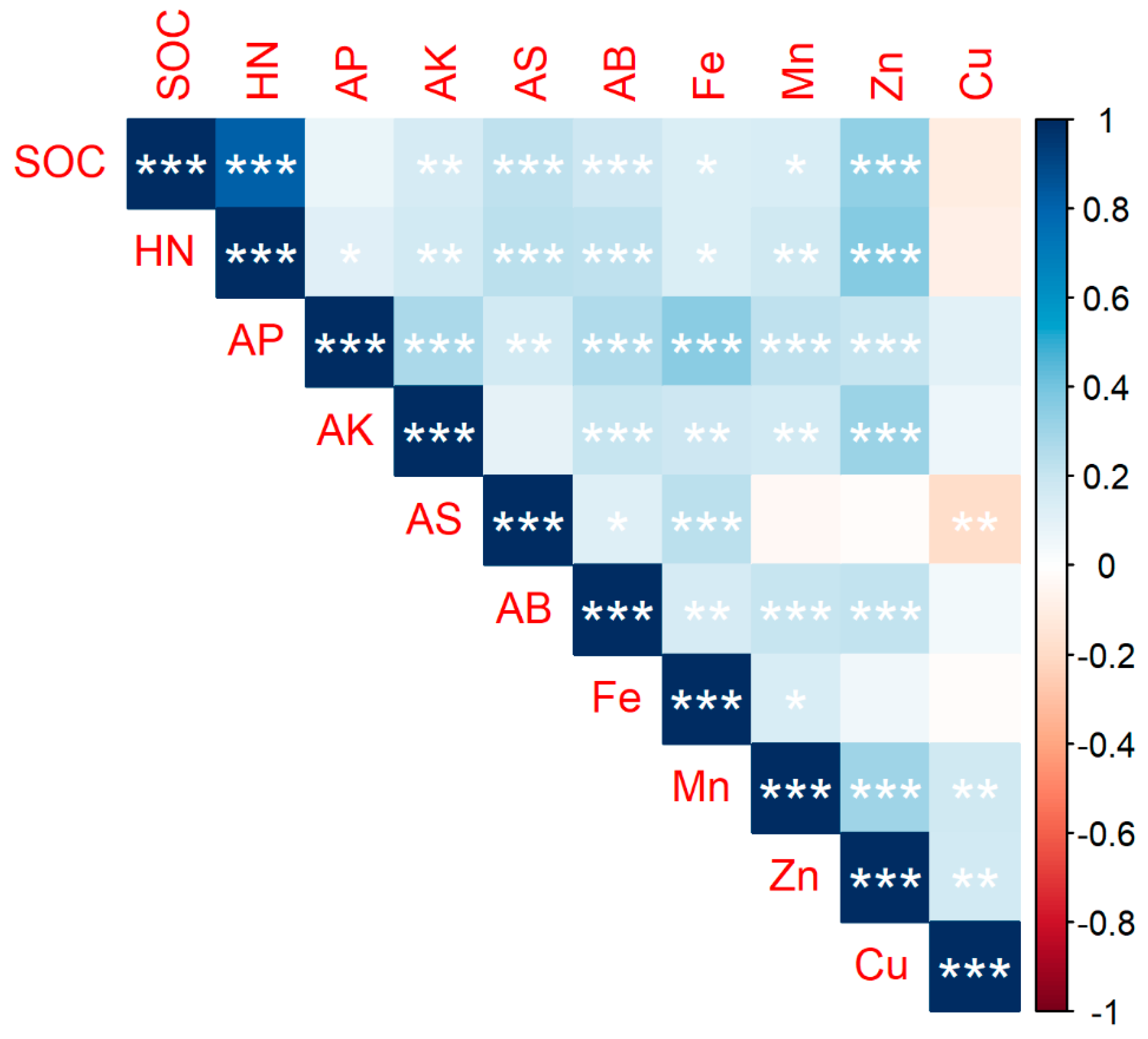
3.1. Correlation Analysis of Soil Physicochemical Properties in Hickory Plantation

Correlation analysis is an effective method to reveal the relationship between soil nutrients (Figure 2). A significant positive correlation was observed among soil organic carbon, hydrolyzed nitrogen, available phosphorus, available potassium, soil available boron, iron, manganese and zinc concentrations, which proved that these nutrients may be affected by similar factors. The highest correlation coefficient was observed between soil organic carbon and hydrolyzed nitrogen concentrations. Copper had correlations with the other nutrients with small correlation coefficients, which indicated that copper may have had different driving factors compared with other nutrients in the soil.

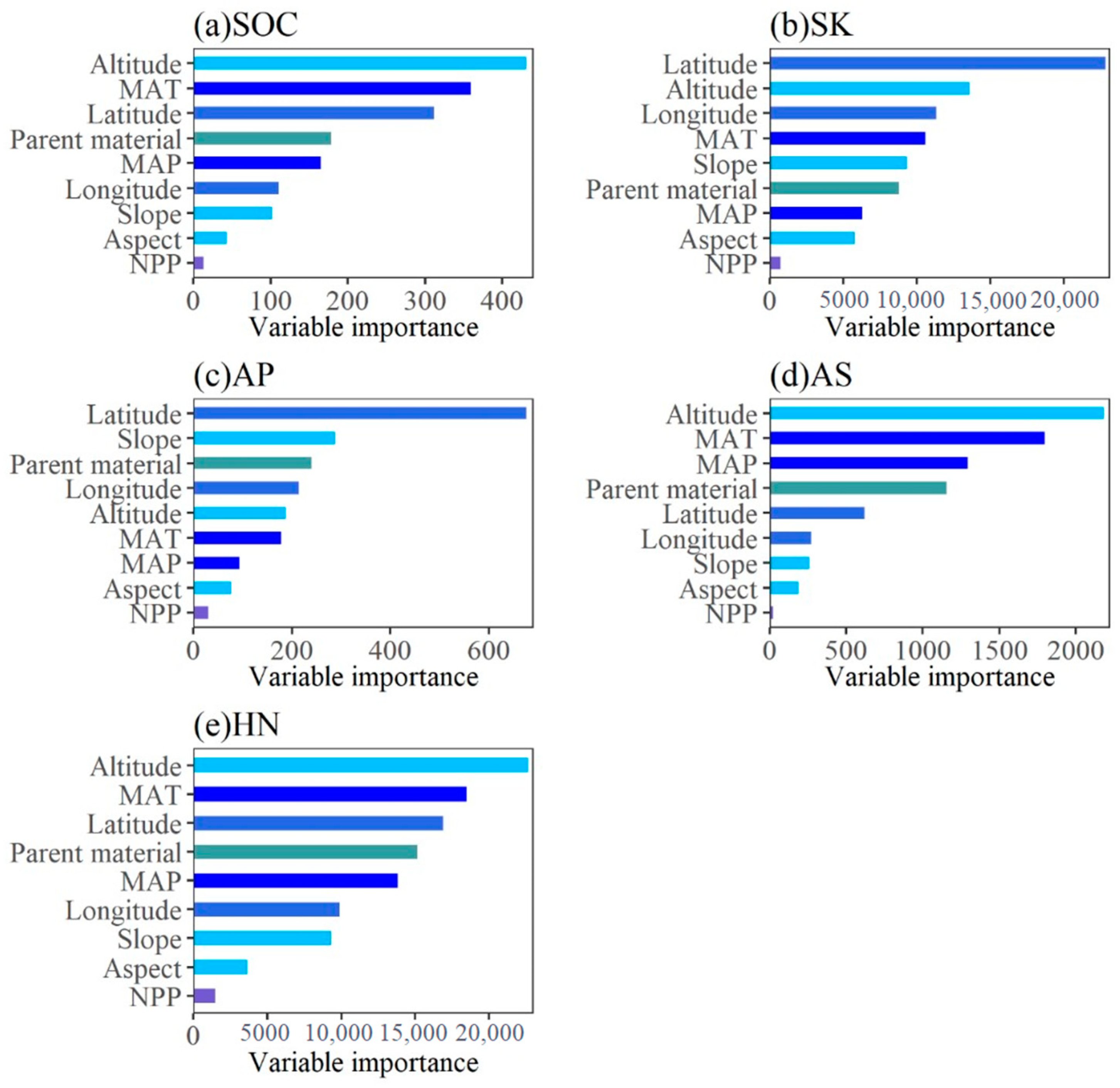
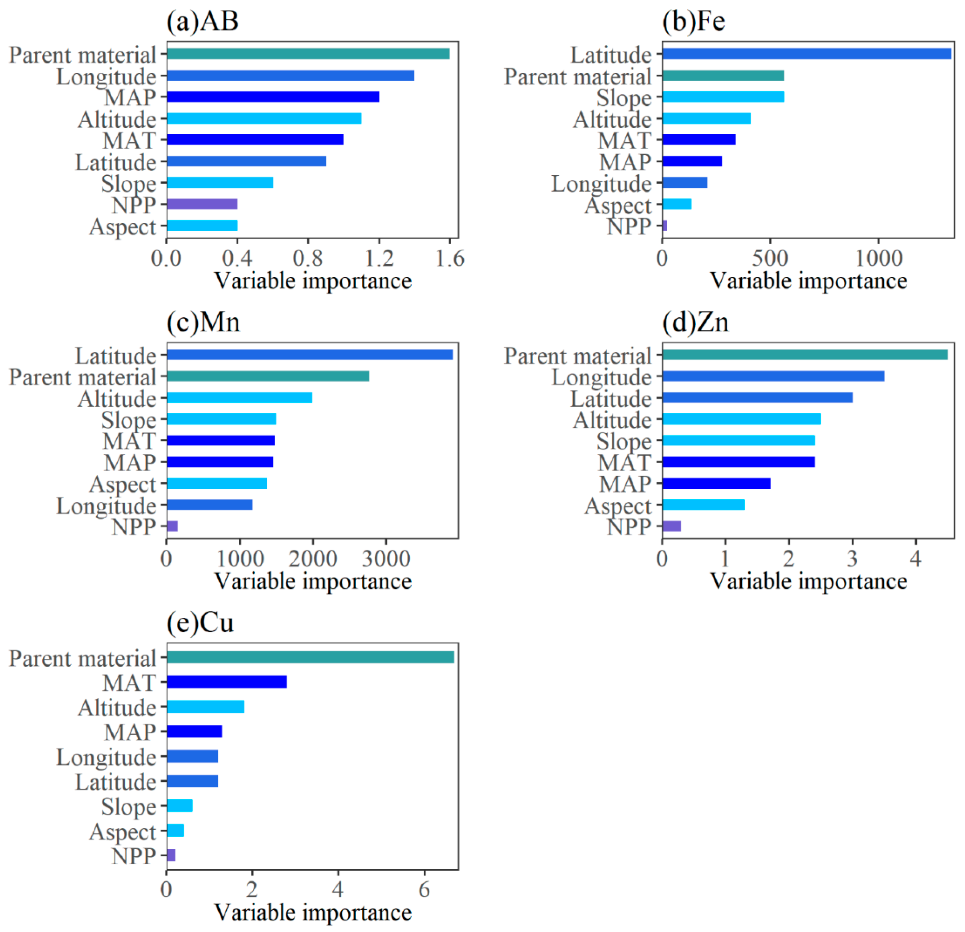
3.2. Performance and Variable Importance of Random Forest Models for Predicting Soil Nutrients in a Hickory Plantation

To optimize the performance of random forest prediction, we selected the parameter combination with the highest goodness of fit, that is, ntree = 5000, mtry = 3, nodesize = 3 (Table S1). In general, the performance of the models was limited. On average, the prediction accuracy was lowest for available phosphorus compared to macronutrient components, namely soil organic carbon, available potassium, hydrolyzed nitrogen, and micronutrients ranging from between 0.60 and 0.80 in R²_oob (

Table 1. Performance of random forest models in the prediction of soil physicochemical properties. (SOC indicates soil organic carbon, SK indicates soil available potassium, AP indicates soil available phosphorus, AS indicates available sulfur, HN indicates soil hydrolyzed nitrogen, AB indicates soil available boron; Fe, Mn, Zn, and Cu indicate soil iron, manganese, zinc, and copper; R²_oob indicates coefficient of determination, RMSE_oob indicates root mean square error, MAE_oob indicates mean absolute error).

Soil Properties	R2oob	RMSEoob	MAEoob
SOC	0.67	1.66	1.02
SK	0.69	10.42	7.92
HN	0.60	11.30	8.65
AP	0.29	1.57	0.98
AS	0.43	4.62	2.36
AB	0.63	0.10	0.07
Fe	0.67	2.54	1.78
Mn	0.77	4.49	3.64
Zn	0.51	0.15	0.11
Cu	0.79	0.15	0.12

). These results suggested that, in the topsoil, the spatial distribution patterns of soil nutrients were highly variable due to small scale variations in input, redistribution, as well as due to the intrinsic random variability of soil nutrients.

Variable importance revealed different dominating influencing features between soil nutrients random forest models (Figure 3 and Figure 4). Net primary productivity aspects were of little importance in the prediction of soil organic carbon, whereas the altitude and mean annual temperature had a strong impact. The level of organic carbon in topsoil is contingent on the inputs of biomass into the soil, which are influenced by climate. The predictors showed similar patterns of variable importance between several macronutrients. Similar to soil organic carbon, altitude and mean annual temperature had a strong impact on the predictions of soil organic carbon. For the prediction of available potassium, hydrolyzed nitrogen, and available sulfur, altitude and mean annual temperature were more crucial than other variables. The macronutrient variables were ranked by climate, parent material, topography, and vegetation. Climate was the most critical predictor for macronutrients, as it determined their spatial distribution. As with macronutrients, the net primary productivity and other aspects of micronutrients were weak predictors within the random forest models. Parent materials were highly influential for micronutrients, as they determined their spatial distribution. The variables were ranked in the order of parent materials, climate, topography, and vegetation. Although certain predictors were more important within a few soil nutrient random forest models, we could not quantitatively determine their functional relationship to soil nutrients. In this respect, the spatial visualization of prediction results were essential toward understanding the driving processes behind soil nutrient predictions.

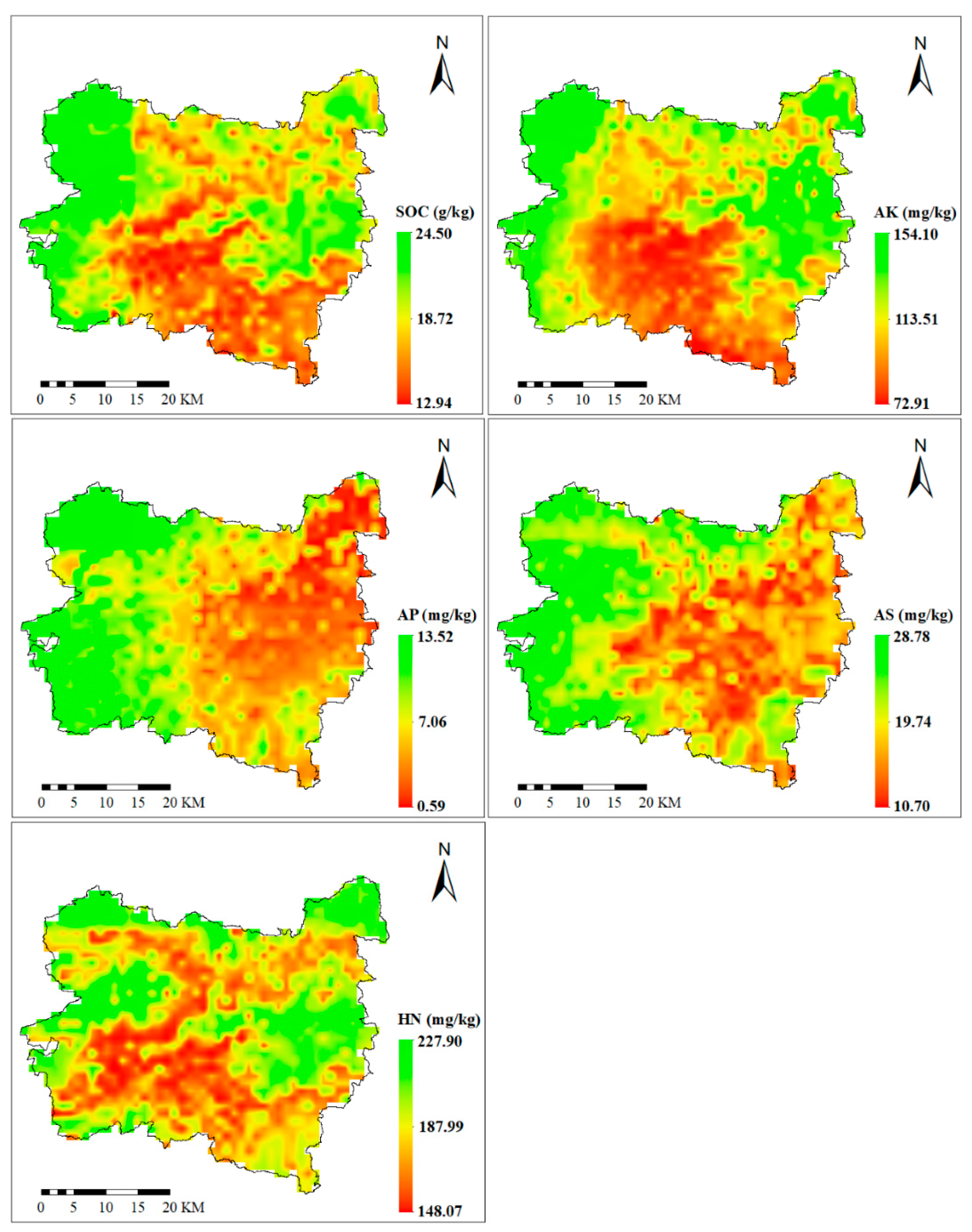
3.3. Spatial Pattern of Soil Nutrients in a Hickory Plantation

The spatial distribution of soil nutrient concentrations in the hickory plantations mapped by the RF model revealed that all of the soil nutrients had obvious spatial patterns (Figure 5 and Figure 6). The concentrations of soil organic carbon, available phosphorus and hydrolyzed nitrogen in the soil had similar spatial distribution patterns, with high concentrations primarily located in the northwest and northeast, and areas of obviously low concentrations in the south. The available potassium exhibited a decreasing trend from west to east. The high-value regions were distributed across the northwest, with the maximum value being 13.52 mg/kg, whereas the concentration in the east was the lowest, as low as 0.59 mg/kg. Low concentrations of available sulfur in the soil were also found in the east, whereas the highest value in the west reached up to 28.78 mg/kg. Generally speaking, in our study, high soil resident macronutrient values were primarily distributed across the western regions, and low values were distributed across the eastern regions, which was consistent with the spatial distribution of the altitude of the west being higher than that of the east.

The soil concentrations of zinc and copper had similar spatial distribution patterns, with high concentrations being located mainly in the center of the hickory plantation, and obviously low concentration areas in the northeast. High concentrations of available boron in soils were found in the west, with low content in the southeast and northeast region, which showed decreasing spatial distribution characteristics, from west to southeast and northeast. The iron concentrations in the northwest and east of the study area were relatively high. The low-value region for manganese was distributed across the southwest, while high-value regions were unevenly distributed.

4. Discussion

There are a myriad of factors that contribute to the spatial variability of soil nutrients, including mean annual temperature, mean annual precipitation, altitude, slope, aspect, net primary productivity, and parent material. Defining the main influencing factors of soil nutrients in hickory plantations is the basis for correctly estimating soil nutrients concentrations and implementing related management measures. In our study, random forest modeling was employed to improve the prediction results, and the optimal settings were selected for each parameter. Through the analysis of each evaluation index, R² was as high as 0.79, and the prediction performance of each nutrient model was enhanced. Variable importance revealed different dominating influencing factors between soil nutrients. As hypothesized, climate was the most important predictor of variation in soil nutrients.

Climate affects soil structure, soil total nitrogen, total soil organic carbon and other nutrient concentrations by affecting soil organic matter composition and microbial activity [36]. Parent materials affect soil nutrient content by influencing soil mechanical composition and material basis [37]. Topography affects the absorbance of solar energy in a given landscape. The effects of slope and aspect on soil nutrients are related to temperature and moisture, and primarily manifested by the sunny aspect being dry, under which the soil organic matter is decomposed more rapidly, with concentrations lower than that under shady conditions [38].

4.1. Mean Annual Temperature, Mean Annual Precipitation and Altitude Control the Spatial Distribution of Soil Nutrients

Correlation analysis revealed that there was a significant positive correlation between nutrients, and the variable importance of soil nutrients was basically the same, which verified that these nutrients may be influenced by similar factors (Figure 2). Climate and altitude drive the spatial distribution of nutrients to a greater degree than do the parent material, slope, and aspect factors. The concentration of soil nutrients is generally negatively associated with temperature and positively associated with the annual mean precipitation [39,40]. Differences in the concentrations of soil nutrients between altitudes might be due to differences in temperature and precipitation. The decrease in temperature with increasing elevation reduces organic matter decomposition rates more than litter production, therefore inducing an accumulation of organic matter [41,42]. The altitude of the west is higher than that of the east, which was consistent with the predicted spatial distribution of macronutrients. Further, the high values of soil nutrients were primarily distributed across the western portion of the hickory plantation. To improve the productivity and yields of hickory, the higher altitude areas in the west should be considered in later management and forest selection, where the elevation range of from 400–800 m is more conducive to the growth of hickory. When temperatures and water parameters are beyond the range required for optimal growth, soil nutrients can be constrained [43,44]. Our models suggested that climate factors outweighed the influences of any other factors, at least in the region and across the environmental gradients that our study encompassed. One possible explanation for this phenomenon is that (to some extent) climate has an overriding influence on large scale patterns in ecosystems, including soil carbon cycling, via its control of plant community composition and productivity [45].

4.2. Effects of Other Factors on Soil Nutrients

In our study, slope also showed a high relative importance in the spatial prediction of soil nutrients, especially in soil available phosphorus and iron. Slope affects runoff, soil moisture concentrations, and the soil erosion rate, which in turn influences soil nutrients [46,47]. As the slope angle increases, the precipitation received per unit area, as well as its infiltration, decreases due to the greater slope area and higher water flow velocity. Meanwhile, the soil moisture concentration is reduced due to the higher runoff and evaporation area [48]. The soil nutrient content on the low slope of acid volcanic rock in the west of the study area is higher than that on the steep slope of mixed sedimentary rock in the northeast of the study area. Consequently, we could not exclude the slope effects even though they were not the most important factor to drive other soil nutrient concentration variabilities in our study. Further research will be required to identify the influences of slope conditions on soil nutrients in hickory plantations. Hypothetically, steeper slopes may likely result in higher risks of runoff and soil loss. The luxuriant vegetation in the flat and gentle slopes at the <15° level generally facilitates the accumulation of soil organic matter and is better suited to hickory growth.

Our study analyzed soil nutrients at a surface depth of 30 cm. The spatial patterns and drivers of deeper subsoils remain unknown and might be important for the production of hickory plantations. However, our results provide a reference for the maintenance and management of soil nutrients in other economic forests. To improve the yields and quality of economic forest, factors such as climate, parent material, elevation, and slope should be taken into consideration. Hickory planting sites should have good illumination, sufficient and uniform rainfall, and a suitable altitude. Soil formed by the weathering of parent rocks that are most suitable for the growth of economic forests should be prioritized. Generally, the slopes of forested lands cannot be too steep.

5. Conclusions

Through the systematic sampling of soils in a typical hickory region, we quantified the relative importance of factors to explain regional variations in its physicochemical properties. Macronutrients and micronutrients in hickory plantations all had obvious spatial patterns. The mean annual temperature, mean annual precipitation, and altitude were found to be the most significant factors for elucidating the spatial variations in soil nutrients. Slope and parent material were also important for explaining the spatial variations in soil nutrients, especially in soil available phosphorus and micronutrients. Aspect and net primary productivity were less important in the prediction of spatial variations for both soil macronutrients and micronutrients but should not be ignored. An improved understanding of the spatial variations and drivers of soil nutrients in plantations will aid in the management of soil nutrients effectively.

References

1. Patil, P. Forest Accounting and Ecological Sustainability. Glob. J. Manag. Bus. Res. 2017, 17, 9–16. [Google Scholar]
2. Littke, K.; Harrison, R.; Zabowski, D.; Briggs, D.; Maguire, D. Effects of Geoclimatic Factors on Soil Water, Nitrogen, and Foliar Properties of Douglas-Fir Plantations in the Pacific Northwest. Forest Sci. 2014, 60, 1118–1130. [Google Scholar] [CrossRef]
3. Grimm, R.; Behrens, T.; Mrker, M.; Elsenbeer, H. Soil organic carbon concentrations and stocks on Barro Colorado Island—Digital soil mapping using Random Forests analysis. Geoderma 2008, 146, 102–113. [Google Scholar] [CrossRef]
4. Liu, Z.; Zhou, W.; Shen, J.; He, P.; Lei, Q.; Liang, G. A simple assessment on spatial variability of rice yield and selected soil chemical properties of paddy fields in South China. Geoderma 2014, 235, 39–47. [Google Scholar] [CrossRef]
5. Yang, R.; Zhang, G.; Liu, F.; Yang, F.; Lu, Y.; Yang, F.; Li, D.; Yang, M.; Zhao, Y. Comparison of boosted regression tree and random forest models for mapping topsoil organic carbon concentration in an alpine ecosystem. Ecol. Indic. 2016, 60, 870–878. [Google Scholar] [CrossRef]
6. Wanshnong, R.; Thakuria, D.; Sangma, C.; Ram, V.; Bora, P. Influence of hill slope on biological pools of carbon, nitrogen, and phosphorus in acidic alfisols of citrus orchard. Catena 2013, 111, 1–8. [Google Scholar] [CrossRef]
7. Elbasiouny, H.; Abowaly, M.; Abu_Alkheir, A.; Gad, A. Spatial variation of soil carbon and nitrogen pools by using ordinary Kriging method in an area of north Nile Delta, Egypt. Catena 2014, 113, 70–78. [Google Scholar] [CrossRef]
8. Roger, A.; Libohova, Z.; Rossier, N.; Joost, S.; Maltas, A.; Frossard, E.; Sinaj, S. Spatial variability of soil phosphorus in the Fribourg canton, Switzerland. Geoderma 2014, 217, 26–36. [Google Scholar] [CrossRef]
9. Xin, Z.B.; Qin, Y.B.; Yu, X.X. Spatial variability in soil organic carbon and its influencing factors in a hilly watershed of the Loess Plateau, China. Catena 2016, 137, 660–669. [Google Scholar] [CrossRef]
10. Jenny, H. Factors of Soil Formation: A System of Quantitative Pedology. N. Y. McGraw-Hill 1941, 50, 7. [Google Scholar]
11. Wang, S.; Jin, X.; Adhikari, K.; Li, W.; Yu, M.; Bian, Z.; Wang, Q. Mapping total soil nitrogen from a site in northeastern China. Catena 2018, 166, 134–146. [Google Scholar] [CrossRef]
12. Saito, H.; Mckenna, S.A.; Zimmerman, D.A.; Coburn, T.C. Geostatistical interpolation of object counts collected from multiple strip transects: Ordinary kriging versus finite domain kriging. Stoch. Environ. Res. Risk Assess. 2005, 19, 71–85. [Google Scholar] [CrossRef]
13. Lacoste, M.; Minasny, B.; Mcbratney, A.B.; Michot, D.; Walter, C. High resolution 3D mapping of soil organic carbon in a heterogeneous agricultural landscape. Geoderma 2014, 214, 296–311. [Google Scholar] [CrossRef]
14. Tesfahunegn, G.B.; Tamene, L.; Vlek, P.L.G. Catchment-scale spatial variability of soil properties and implications on site-specific soil management in northern Ethiopia. Soil Tillage Res. 2011, 117, 124–139. [Google Scholar] [CrossRef]
15. Veronesi, F.; Schillaci, C. Comparison between geostatistical and machine learning models as predictors of topsoil organic carbon with a focus on local uncertainty estimation. Ecol. Indic. 2019, 101, 1032–1044. [Google Scholar] [CrossRef]
16. Liaw, A.; Wiener, M. Classification and Regression with RandomForest. R. News 2002, 23, 18–22. [Google Scholar]
17. Heung, B.; Bulmer, C.E.; Schmidt, M.G. Predictive soil parent material mapping at a regional-scale: A Random Forest approach. Geoderma 2014, 214, 141–154. [Google Scholar] [CrossRef]
18. Zhu, J.; Wu, W.; Liu, H.B. Environmental variables controlling soil organic carbon in top- and sub-soils in karst region of southwestern China. Ecol. Indic. 2018, 90, 624–632. [Google Scholar] [CrossRef]
19. Wu, W.F.; Lin, H.P.; Fu, W.J.; Penttinen, P.; Li, Y.F.; Jin, J.; Zhao, K.L.; Wu, J.S. Soil Organic Carbon Content and Microbial Functional Diversity Were Lower in Monospecific Chinese Hickory Stands than in Natural Chinese Hickory–Broad-Leaved Mixed Forests. Forests 2019, 10, 357. [Google Scholar] [CrossRef] [Green Version]
20. Shen, Y.F.; Qian, J.F.; Zheng, X.P.; Yuan, Z.Q.; Huang, J.Q.; Wen, G.S.; Wu, J.S. Spatial-temporal variation of soil fertility in chinese walnut (Carya cathay ensis ) plantation. Sci. Silvae Sin. 2016, 52, 1–12. [Google Scholar] [CrossRef]
21. Huang, X.Z.; Huang, J.Q.; Chen, D.H.; Lv, J.Q.; Wu, J.S. Comparison on Soil Physical and Chemical Properties at Different Vertical Zones of Carya cathayensis Stands. J. Zhejiang For. Sci. Technol. 2010, 30, 23–27. [Google Scholar]
22. Blake, G.R. Particle density. Methods Soil Anal. 2008, 1, 504–505. [Google Scholar]
23. Guitian, F.; Carballas, T. Técnicas de Anâlisis de suelos, 2, a ed. Pico Sacro, Santiago de Compostela. 1976. Available online: https://doi.org/10.1097/00010694-197609000-00009 (accessed on 10 February 2022).
24. Nelson, D.W. Total carbon, organic carbon, and organic matter. Methods Soil Anal. 1996, 9, 961–1010. [Google Scholar]
25. Jackson, M. Soil Chemical Analysis—An Advanced Course; UW-Madison Libraries Parallel Press: Madison, WI, USA, 2005. [Google Scholar]
26. Wu, J.S.; Lin, H.P.; Meng, C.F.; Jiang, P.K.; Fu, W.J. Effects of intercropping grasses on soil organic carbon and microbial community functional diversity under Chinese hickory (Carya cathayensis Sarg.) stands. Soil Res. 2014, 52, 575. [Google Scholar] [CrossRef]
27. Smith, A.M.; Anderson, G. The relationship between the boron contents of soils and swede roots. J. Sci. Food Agric. 1955, 6, 157–162. [Google Scholar] [CrossRef]
28. Agricultural Chemistry Committee of China. Conventional Methods of Soil and Agricultural Chemistry Analysis; Science Press: Beijing, China, 1983. [Google Scholar]
29. Null, R.; Team, R.; Null, R.; Writing, T.C.; Null, R.; Team, R.; Null, R.; Core, R.; Team, R.; Team, R. R: A language and environment for statistical computing. Computing 2011, 1, 12–21. [Google Scholar]
30. Díaz-Uriarte, R.; Alvarez de Andrés, S. Gene selection and classification of microarray data using random forest. BMC Bioinform. 2006, 7, 3. [Google Scholar] [CrossRef] [PubMed] [Green Version]
31. Prasad, A.M.; Iverson, L.R.; Liaw, A. Newer classification and regression tree techniques: Bagging and random forests for ecological prediction. Ecosystems 2006, 9, 181–199. [Google Scholar] [CrossRef]
32. Rodriguez-Galiano, V.F.; Ghimire, B.; Rogan, J.; Chica-Olmo, M.; Rigol-Sanchez, J.P. An assessment of the effectiveness of a random forest classifier for land-cover classification. ISPRS J. Photogr. Remote Sens. 2012, 67, 93–104. [Google Scholar] [CrossRef]
33. Huang, X.; Cui, C.; Hou, E.; Li, F.; Liu, W.; Jiang, L.; Luo, Y.; Xu, X. Acidification of soil due to forestation at the global scale. For. Ecol. Manag. 2022, 505, 119951. [Google Scholar] [CrossRef]
34. Mangla, R.; Kumar, S.; Nandy, S. Random forest regression modelling for forest aboveground biomass estimation using RISAT-1 PolSAR and terrestrial LiDAR data. In Proceedings of the Lidar Remote Sensing for Environmental Monitoring XV, New Delhi, India, 8 December 2016. [Google Scholar]
35. ESRI. What is ArcGIS? 2002. Available online: http://bases.bireme.br/cgi-bin/wxislind.exe/iah/online/?IsisScript=iah/iah.xis&src=google&base=REPIDISCA&lang=p&nextAction=lnk&exprSearch=35663&indexSearch=ID (accessed on 10 February 2022).
36. Neff, J.C.; Hooper, D.U. Vegetation and climate controls on potential CO2, DOC and DON production in northern latitude soils. Glob. Change Biol. 2002, 8, 872–884. [Google Scholar] [CrossRef]
37. Foroughifar, H.; Jafarzadeh, A.A.; Torabi, H.; Pakpour, A.; Miransari, M. Using Geostatistics and Geographic Information System Techniques to Characterize Spatial Variability of Soil Properties, Including Micronutrients. Commun. Soil Sci. Plant Anal. 2013, 44, 1273–1281. [Google Scholar] [CrossRef]
38. Zhang, Z.M.; Zhou, Y.C.; Wang, S.J.; Huang, X.F. The soil organic carbon stock and its influencing factors in a mountainous karst basin in P. R. China. Carbonates Evaporites 2018, 34, 1031–1043. [Google Scholar] [CrossRef]
39. Yang, Y.H.; Fang, J.Y.; Wenhong, M.A.; Smith, P.; Wang, W. Soil carbon stock and its changes in northern China’s grasslands from 1980s to 2000s. Glob. Change Biol. 2010, 16, 3036–3047. [Google Scholar] [CrossRef]
40. Hobley, E.; Wilson, B.; Wilkie, A.; Gray, J.; Koen, T. Drivers of soil organic carbon storage and vertical distribution in Eastern Australia. Plant Soil 2015, 390, 111–127. [Google Scholar] [CrossRef]
41. Choudhury, B.U.; Fiyaz, A.R.; Mohapatra, K.P.; Ngachan, S. Impact of Land Uses, Agrophysical Variables and Altitudinal Gradient on Soil Organic Carbon Concentration of North-Eastern Himalayan Region of India. Land Degrad. Dev. 2016, 27, 1163–1174. [Google Scholar] [CrossRef]
42. Tsozué, D.; Nghonda, J.P.; Tematio, P.; Basga, S.D. Changes in soil properties and soil organic carbon stocks along an elevation gradient at Mount Bambouto, Central Africa. Catena 2019, 175, 251–262. [Google Scholar] [CrossRef]
43. Huang, M.T.; Piao, S.L.; Ciais, P.; Peñuelas, J.; Wang, X.H.; Keenan, T.F.; Peng, S.S.; Berry, J.A.; Wang, K.; Mao, J.F.; et al. Air temperature optima of vegetation productivity across global biomes. Nat. Ecol. Evol. 2019, 3, 772–779. [Google Scholar] [CrossRef] [PubMed]
44. Eamus, D. How does ecosystem water balance affect net primary productivity of woody ecosystems? Funct. Plant Biol. 2003, 30, 187–205. [Google Scholar] [CrossRef] [PubMed]
45. Sinoga, J.D.R.; Pariente, S.; Diaz, A.R.; Murillo, J.F.M. Variability of relationships between soil organic carbon and some soil properties in Mediterranean rangelands under different climatic conditions (South of Spain). Catena 2012, 94, 17–25. [Google Scholar] [CrossRef]
46. Johnson, C.E.; Ruiz-Mendez, J.J.; Lawrence, G.B. Forest Soil Chemistry and Terrain Attributes in a Catskills Watershed. Soil Sci. Soc. Am. J. 2000, 64, 1804–1814. [Google Scholar] [CrossRef]
47. Wang, H.J.; Shi, X.Z.; Yu, D.S.; Weindorf, D.C.; Huang, B.; Sun, W.X.; Ritsema, C.J.; Milne, E. Factors determining soil nutrient distribution in a small-scaled watershed in the purple soil region of Sichuan Province, China. Soil Tillage Res. 2009, 105, 300–306. [Google Scholar] [CrossRef]
48. Florinsky, I.V. Digital Terrain Analysis in Soil Science and Geology, 2nd ed.; Academic Press: Cambridge, MA, USA, 2016; pp. 377–385. [Google Scholar]
Figure 1. Location of the study area and soil samples.
Forests 13 00457 g001
Figure 2. Correlation analysis of soil physicochemical properties in hickory plantations. (SOC indicates soil organic carbon, SK indicates soil available potassium, AP indicates soil available phosphorus, AS indicates available sulfur, HN indicates soil hydrolyzed nitrogen, AB indicates soil available boron. * Correlation is significant at the 0.05 level, ** Correlation is significant at the 0.01 level, *** Correlation is significant at the 0.001 level).
Forests 13 00457 g002
Figure 3. Variable importance of predictors in forecasting soil physicochemical properties. (MAT indicates mean annual temperature, MAP indicates mean annual precipitation, NPP indicates net primary productivity). (a) SOC indicates soil organic carbon concentration; (b) SK indicates soil available potassium concentration; (c) AP indicates soil available phosphorus concentration; (d) AS indicates available sulfur concentration; (e) HN indicates soil hydrolyzed nitrogen concentration.
Forests 13 00457 g003
Figure 4. Variable importance of predictors in forecasting soil physicochemical properties. (MAT indicates mean annual temperature, MAP indicates mean annual precipitation, NPP indicates net primary productivity). (a) AB indicates soil available boron concentration; (b) Fe indicates soil iron concentration; (c) Mn indicates soil manganese concentration; (d) Zn indicates soil zinc concentration; (e) Cu indicates soil copper concentration.
Forests 13 00457 g004
Figure 5. Mapping spatial distribution maps of macronutrients in soils. (SOC indicates soil organic carbon, SK indicates soil available potassium, AP indicates soil available phosphorus, AS indicates available sulfur, HN indicates soil hydrolyzed nitrogen).
Forests 13 00457 g005
Figure 6. Spatial distribution maps of micronutrients in soils. (AB indicates soil available boron; Fe, Mn, Zn, and Cu indicate soil iron, manganese, zinc, and copper).
Forests 13 00457 g006