Abstract
Choosing the ideal number of rotations of planted forests under a silvicultural management regime results in uncertainties in the cash flows of forest investment projects. We verified if there is parity in the Eucalyptus wood price modeling through fractional Brownian motion and geometric Brownian motion to incorporate managerial flexibilities into investment projects in planted forests. We use empirical data from three production cycles of forests planted with Eucalyptus grandis × E. urophylla in the projection of discounted cash flows. The Eucalyptus wood price, assumed as uncertainty, was modeled using fractional and geometric Brownian motion. The discrete-time pricing of European options was obtained using the Monte Carlo method. The root mean square error of fractional and geometric Brownian motions was USD 1.4 and USD 2.2, respectively. The real options approach gave the investment projects, with fractional and geometric Brownian motion, an expanded present value of USD 8,157,706 and USD 9,162,202, respectively. Furthermore, in both models, the optimal harvest ages execution was three rotations. Thus, with an indication of overvaluation of 4.9% when assimilating the geometric Brownian motion, there is no parity between stochastic processes, and three production cycles of Eucalyptus planted forests are economically viable.
1. Introduction
When incorporating the real options approach in an analysis of forest projects, the modeling of the underlying asset’s price is one of the main issues to be analyzed, for which some models are assumed. These models must be able to describe the price trajectory of the underlying asset without the need to adopt unrealistic assumptions of the data, such as temporal independence. As the calculations are based on time series of asset prices, time is the first source of dependence on the data.
Statistical tests, such as the GPH estimate [1], allow proving the existence of a true long memory. Thus, the quality of the modeling is accentuated by allowing the correlation between the impacts of crises and financial stress and the behavior of the price of biological assets such as wood. According to observations by Niquidet and Sun [2], many studies focused on the evaluation of the hypotheses of stationarity I (0) and non-stationarity I (1) of the time series, including in the forest scope.
According to Ahmadian and Rouz [3], the properties of self-similarity and long-range dependence that may be present in this type of series are often ignored. In these conditions, the fractional Brownian motion (FBM) is suitable for financial mathematical modeling [4]. This is because the Gaussian random field with stationary increments can admit directions in which its regularity is greater, allowing fractal analysis to increase the accuracy of diagnoses [5].
Furthermore, FBM supports self-similarity and stationary increments, in addition to displaying long memory. These compact properties help characterize real-world phenomena [6]. The estimation of the true long memory factor is essential for regulatory authorities to seek to maintain financial stability and public policy management [7], as well as providing subsidies to forest managers when undertaking forest investment projects. FBM has also shown a better performance in modelling the commodity market [8].
Given the inconstancy of the forest economy [9], the underlying non-Markovian stochastic process provides natural subsidies of analysis to capture ubiquitous complex sequences of fluctuations [10]. Furthermore, this aligns with the companies’ investment strategy and the environments where they find value creation from available options is promoted [11]. After all, the economic success of any investment project lies in realizing the strategic value of the business, which gives companies, especially forest companies, competitive advantages [12]. Thus, the opportunity to exercise a forestry investment decision, such as the number of rotations, under certain silvicultural management systems, provides value creation to the forest investment project since the value of the investment option is determined by the interaction between the market uncertainty and the investment strategy [13].
In Brazil, Eucalyptus is a fast-growing hardwood, capable of developing under different climatic conditions and presenting chemical, physical, and mechanical properties that serve different industrial niches. In the pulp and paper industry, the chemical properties differentiate the pulp from Eucalyptus. In the production of wood panels, the short and resistant fibers favor the transformation of raw material. In building construction, the mechanical properties are highlighted, such as compression, tension, and shear resistance [14,15,16,17]. Thus, these wood specificities and its employability make the final price of wood a relevant premise for analysis of forestry investment, given that the price can be considered the main source of uncertainty in projects of Eucalyptus planted forests.
Stochastic modeling can be segmented into long-range dependence phenomena and those that consider stochastic differential equations with Markov switching. The emphasis on fractional Brownian motion favors the modeling of biological assets price trajectories and allows the correlation of their disjoint increments, identifying persistent behaviors in different periods. Econometric tests that evaluate the normality of data distribution, trend, autocorrelation, stationarity, and estimation of the fractional differential guide the stochastic processes that best perform the prediction of these prices [8,18,19,20].
In this sense, the adoption of the FBM to model the price of biological assets can surpass the quality of model adjustment, such as the geometric Brownian motion (GBM), as it considers self-similarity and the existence of true long memory that will result in more reliable subsidies for decision-making. Therefore, the modeling of the price of the underlying asset by means of the FBM is justified by allowing the incorporation of managerial flexibility in decision-making and enabling the creation of value for forest-based companies through investments in biological assets, with appropriate econometric treatment of biological assets.
That said, we verified if there is parity in the Eucalyptus wood price modeling through the FBM and the GBM to incorporate managerial flexibilities into investment projects in planted forests.
2. Materials and Methods
2.1. Species and Silvicultural Management
Our study was based on a forest planted with Eucalyptus grandis × E. urophylla, spaced 3 m × 2 m, in 3615 hectares belonging to a forest-based industry located in the Midwest region of the state of São Paulo, Brazil, to produce particulate wood panels. Therefore, we considered three consecutive rotations, that is, three production cycles of seven years each, under silvicultural management (Table 1).

Table 1.
Technical parameters of silvicultural management.
2.2. Analysis of the Timber Price Time Series
We used a time series of the monthly prices of Eucalyptus wood from January 2011 to June 2018. Further details are provided in Supplementary Materials (Table S1). To verify the behavior of the time series, we applied econometric tests of normality, trend, stationarity, autocorrelation, and linearity [21,22]. With the aid of the R [23] programming language, we used the tests:
- Jarque Bera test [24] with the null hypothesis of normal data distribution, package tseries;
- Cox Stuart test [25] with the null hypothesis that the time series has a trend, package randtests;
- Phillips-Perron test [26] with the null hypothesis of unit root, I (1), package aTSA;
- Kwiatkowski–Phillips–Schmidt–Shin (KPSS) test [27], with the null hypothesis of stationarity, I (0), package aTSA;
- GPH estimate [1] of the fractional difference parameter (d), package fracdiff.
2.3. Model of the Underlying Asset Price
When we have estimated the fractional difference parameter, we can estimate the Hurst exponent (H) of a series of logarithmic price returns. We estimated the volatility (σ) and drift (α) of the price of Eucalyptus wood returns according to Equations (1) and (2):
where is the variance of a series of logarithmic returns, and is Hurst coefficient, considering the fractional differential factor;
where is the arithmetic mean of a series of logarithmic returns.
Thus, we assume that the price of the underlying asset can be modeled as an FBM (Equation (3)), according to Manley and Niquidet [18]:
where is the fractional Gaussian noise.
To establish a comparison, we performed the modeling of the underlying asset following the GBM (Equation (4)), according to Miranda et al. [28]. Thus, we tested the difference between the models using Wilcoxon rank sum test [29], with a significance level of 5%. Note that for GBM, the fractional difference parameter is 0.5. Therefore, for Hurst, the coefficient is zero.
where is the random error with standard normal distribution.
Furthermore, we defined the best fit for Eucalyptus wood price modeling according to root mean square error (RMSE), used as a performance indicator. Once associated, we used the coefficient of determination (R2) as a performance measure.
2.4. Expected Cash Flow from the Forest Investment Project
The remuneration for the use of the land is the opportunity cost that the producer has due to the development of a culture to the detriment of another [30]. This is a premise value of the bare land for reforestation, which is based on the region covered by the study, according to data provided by the Institute of Agricultural Economics [31].
The monetary value of the exhaustion of biological assets and deductions from taxes were weighted in the period in which the flat cut occurred due to the generation of revenues. Therefore, we based the taxation framework of the forestry project on the current legislation. According to Brazil [32], Law N°. 9430 provides for federal tax legislation in the tax regime of real profit, which considers the generation of gross revenue higher than USD 5399.
Therefore, the income tax rate was 25%, while the social contribution on net income was 9%. In addition, we deducted 1.65% referring to the Social Integration Program and 7.6% inherent to the contribution for social security financing.
We designed the expected cash flow (Equation (5)) for a 21-year planning horizon, with the disbursable expenses from silvicultural treatment. Further details are provided in Supplementary Materials (Table S2), which are: mowing, butchery, insecticides, chemical pesticides, chemical weeding, mechanized liming, subsoiling, digging, planting, replanting, irrigation, fence reforms, transportation of inputs, manual and mechanical fertilization, the opening of drains, maintenance of firebreaks Eucalyptus, and elimination of Eucalyptus shoots.
where is the cash flow at age in price state , is the volume of wood at age , is the price of wood at age , is the sum of deductions from PIS, COFINS, is the capital expenditure on silvicultural investments, is the exhaustion, is the remuneration for the use of the land, and is taxation.
2.5. Discount Rate over Forest Investment Project Estimate
According to Brigham and Houston [33], using the weighted average cost of capital (WACC), we estimated the discount rate over forest investment project life (Equation (6)) considering the participation of third-party capital and equity. We also incorporated the tax benefit of interest using the cost of capital after taxes and market risks.
where is the discount rate, is the shareholder’s capital cost, is the creditor’s capital cost, is the share capital of the shareholders, and is the share capital of creditors.
Thus, we computed the rate for the shareholder’s capital cost using the capital asset pricing model (CAPM) based on Baker and English [34] added to country risk based on Bai and Green [35], given in Equation (7):
where is the risk-free rate of return, is the systematic market risk coefficient of the forestry sector, is the expected rate of return of the forestry market portfolio, is the market-risk premium, and is the country-risk premium in Brazil.
We emphasize that the risk-free rate was based on the historical series provided by the Department of the Treasury T-Bonds [36] since 1962 with a maturity term of ten years, commonly used by financial analysts [37]. Therefore, the predilection for longer periods for each variable results in the absence of any trend over time [38].
For the systematic risk coefficient of the market, we estimated the beta of the wood and pulp sector through publicly traded companies, which had shares traded in B3 S.A.–Brasil, Bolsa, Balcão [39]. This includes Dexco S.A., Eucatex S.A. Indústria e Comércio, Klabin S.A., and Suzano S.A. We assumed the S&P Global Timber & Forestry index as a market-risk premium, provided by S&P Dow Jones Indices [40].
In determining the traditional net present value of the investment project (Equation (8)), we subtracted the present value of costs from the present value of benefits:
where is the net present value, is the number of periods, is the discount rate of return that could be earned from an investment in the financial markets with similar risk, and is the cash inflow at moment t.
2.6. Pricing of Options Using the Monte Carlo Technique
The choice of the ideal rotation numbers can be solved using the Monte Carlo methodology since it is a flexible approach for the calculation of option values. It also has a specific use in fields such as forest management. Above all, it can be posed as an expectation-maximization problem given in Equation (9) [41]:
where is the expected future value for each rotation due to the maximum expected discounted cash flow for each rotation with N being a multiple of 7.
Therefore, using the Ibáñez and Zapatero [42] approach, we established that the continuation value and the adoption of a new rotation consist of the ideal exercise value frontier. Furthermore, by adapting the algorithm registered by the authors (Equation (10)), we performed the inverse recursion approach with the maximum limit defined for three consecutive rotations, that is, years.
where represents the total number of simulated price paths.
We performed the Monte Carlo simulation of discounted cash flows for each rotation based on the simulation of the price of the underlying asset, which followed the distributions of the FBM model using the R [23] and long memo package, generating 50,000 price paths. The real option value (ROV), which we concurrently considered in the analysis of the expanded present value, resulted from the difference between the expanded present value (EPV) and the present value without flexibility (Equation (11)):
where is the traditional present value.
3. Results
3.1. Modeling the Price of the Underlying Asset
We rejected the first tested hypothesis of data normality (p-value of 0.004) for our time series of Eucalyptus wood price, and we found that the nonparametric time series has a trend (p-value of 5.684e−14). Consequently, the Phillips-Perron test with the hypothesis that the time series with drift and trend has a unit root attested that our series is non-stationary, with a p-value of 0.43.
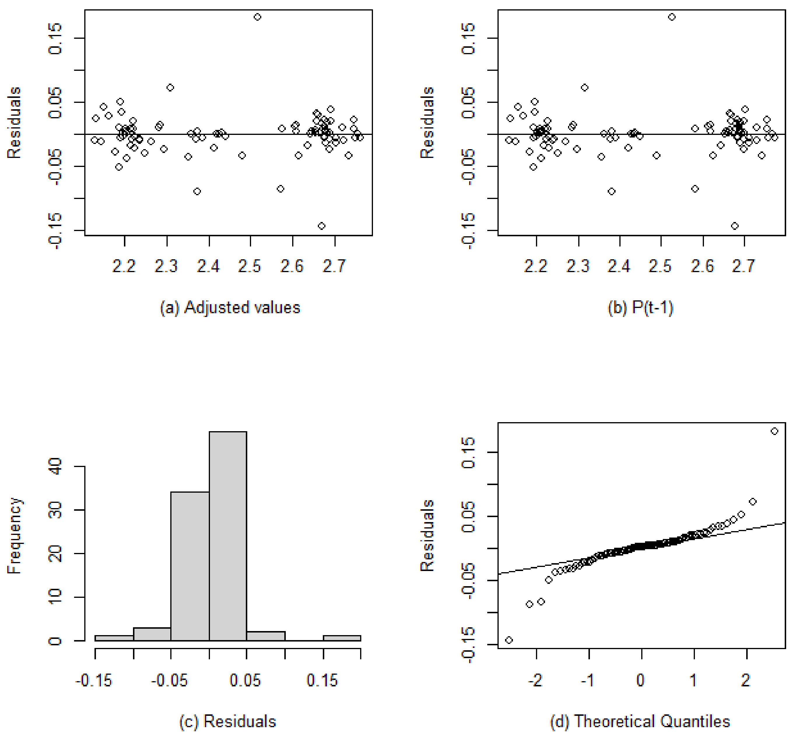
With the performance of the regression analysis, we found that the price of Eucalyptus wood at time significantly influences the price at time t (b = 0.9915), with a t-value of 59.91. Therefore, the quality of the regression adjustment was verified through the hypothesis of normality of the residuals. The Jarque Bera test was rejected with a p-value of 2.2e−16, suggesting that the residuals are not random. Therefore, another factor that influences the dependent variable was not considered in the adjustment (Figure 1).
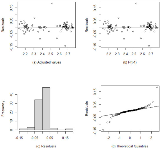
Figure 1.
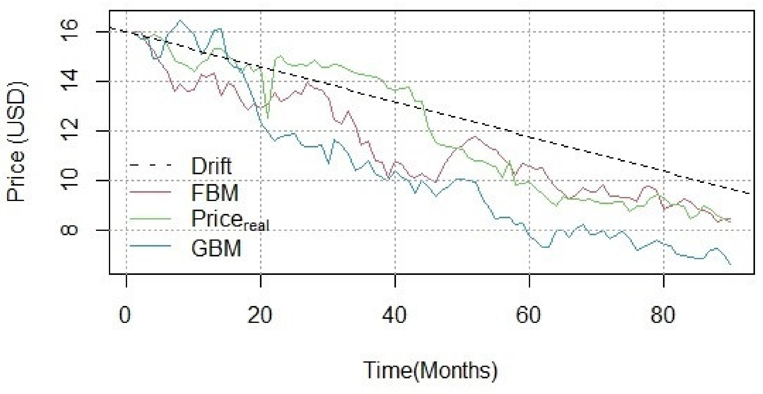
Analysis of regression residuals, with (a) diagram for a residual dispersion and adjusted values; (b) scatter plot of the residuals against the predicted values; (c) residual histogram; (d) dot plot of sample quantiles against theoretical quantiles from the standard normal distribution. Then, through the KPSS test, we found that our time series has a true long memory (p-value of 0.1). Therefore, using the Geweke and Potter-Hudak (GPH) estimate for our time series of the price of Eucalyptus wood , we obtained the value 0.93 of true long memory or fractional difference (d). This resulted in the Hurst coefficient to 0.43 for the differentiated series in demonstrating the historical series behavior of the Eucalyptus wood price when modeled through stochastic models. Figure 2 was plotted, representing the evolution of Eucalyptus wood prices following the fractional Brownian motion and the evolution through the geometric Brownian motion. The dashed line represents the slightly negative trend in prices.
Thus, the best performance in modeling the price of Eucalyptus wood was inferred to FBM, mainly due to the root mean square error (RMSE) of USD 1.4, compared to the RMSE of USD 2.2 of the GBM. In addition, the coefficient of determination (R2) is added, which explained 79.4% of the variation in the price of Eucalyptus wood when modeled by the FBM, while 79.2% by the GBM.
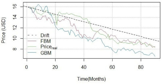
Figure 2.
Simulations of the evolution of Eucalyptus wood prices following the fractional Brownian motion and the evolution through the geometric Brownian motion. The dashed line represents the slightly negative trend in prices.
Figure 2.
Simulations of the evolution of Eucalyptus wood prices following the fractional Brownian motion and the evolution through the geometric Brownian motion. The dashed line represents the slightly negative trend in prices.
3.2. Discount Rate for the Forest Investment Project
Due to the sensitivity of the capital asset pricing model in describing the perception of the risk of investing in a company, especially in the forestry sector, we measured the return required by shareholders at 10.5%, with a risk-free rate of 5.5%. In addition, the systematic risk coefficient of the market, re-leveraged, was 0.42, while the market-risk premium resulted in an annualized return of 7.8%.
As the risk-free rate, the 4.1% risk premium for Brazil was the geometric average of debt securities issued by emerging countries since 1994. However, for the accuracy of creditors, the required return was 9.1%, with a spread of 3.6% for customer default. This is because Brazil had a speculative credit rating (BA2) during the study period. Thus, the opportunity cost rate of the forest investment project was 8.6%, with 34% of the income tax rate, according to the taxation in force in the country. In comparison, it was 43% of the participation of the capital of creditors.
3.3. Valuation of the Forest Investment Project
With the execution of several simulations using the Monte Carlo technique, the model outputs are probability distributions, intending to support the forest manager in choosing the specific value [43]. Therefore, the simulations with the price following the FBM or GBM returned optimal harvest ages of three rotations ordered consecutively, such as IF, CFI, and CFII.
By modelling the price following the FBM, the result of the sum of the simulated averages in 50,000 paths for each rotation with respect to the silvicultural management adopted in each cycle is presented in Table 2. It returned the expanded present value (EPV) of USD 8,157,706, which increased 55.6% to the traditional present value of USD 3,618,678.
Table 2.
Descriptive statistics of Monte Carlo simulation for investment projects of three consecutive rotations, with Eucalyptus wood price following fractional Brownian motion.
For the modeling of the price following the GBM, the expanded present value resulting from the sum of the simulated averages (Table 3) for each rotation was USD 9,162,202, an increase of 60.5% to the traditional present value.
Table 3.
Descriptive statistics of the Monte Carlo simulation for the investment projects of the three consecutive rotations, with the price of Eucalyptus wood following the geometric Brownian motion.
Thus, with the estimated kurtosis and skewness coefficients, the distributions were classified as leptokurtic and symmetrical since a comparison was made between the asymmetry and slenderness of the distributions with the standard behavior of the theoretical normal distribution.
3.4. Impact of the Choice of Wood Price Modeling on the Final Value of the Forest Investment Project
The different modeling of the price of Eucalyptus wood, FBM or GBM, resulted in added value to the forest investment project, making its execution viable since the net present value with flexibility was higher than zero. The traditional approach resulted in a deficit of USD 1,538,862 due to the capital expenditure (CAPEX) of USD 5,157,540.
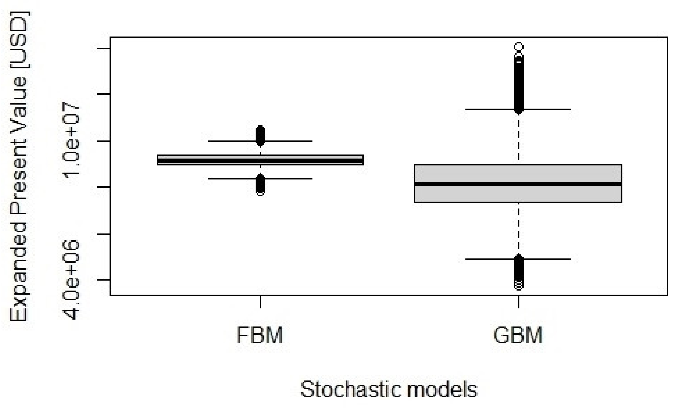
With the modeling of the price of Eucalyptus wood through the GBM, there was an increase of 4.9%, as an exercise premium of optimal harvest ages of the two European options with maturities of 7 and 14 years, consecutively, compared to the modeling through the FBM. The difference between the distributions of the expanded present value for FBM and GBM was statistically significant (Figure 3), attested by the Wilcoxon rank sum test, with a p-value less than 2.2 × 10⁻¹⁶.

Figure 3.
Boxplot of the expanded present value for stochastic models fractional Brownian motion and geometric Brownian motion, representing the difference between the distributions.
4. Discussion
Commodity prices are analyzed under the hypothesis of reversion to average [44,45], Pindyck [46] found that the reversion of the average can often only be proven for time series over 100 years old. Therefore, as the analysis period was 90 months, another test was adopted to confirm the non-stationary condition of the series, known as the Kwiatkowski-Phillips-Schmidt-Shin (KPSS) test. With a hypothesis of stationarity I (0), it is possible to verify if a series is I (d) or if its second difference follows an I (0) process, identifying a true long memory against spurious long memory [2]. This is due to the variations in the price of the underlying asset, that is, in the price of Eucalyptus wood for forest investment projects. It sometimes follows a repetitive pattern that has direct implications on the choice of the adopted silvicultural management. Therefore, it affects the adequacy of forestry policies [2], as well as tax policies applicable to the sector.
Thus, when verifying the behavior of the historical series of the price of Eucalyptus wood, subsidy to the choice of the best mathematical adjustment is achieved. As an example, the estimation of the fractional differential factor, for the series of the price of Eucalyptus wood in a country with an emerging economy, was 0.93.
Estimates of the fractional differential factor for other wood species were made, as for Pinus radiata, in a study developed in New Zealand by Manley and Niquidet [18], obtaining a value of 0.78. The series of data comprised in the range of the year 1973 to 2016. In addition to Niquidet and Sun [2] for wood prices in North America, the fractional differential factor varied between 0.64 and 0.81. The studies that deal with unit root analysis focused on validating the hypotheses of stationarity and non-stationarity. Still, there are shocks caused by the escape from inside the markets during periods of crisis and financial stress [47].
Indeed, for the price of wood, Manley and Niquidet [18] found from a New Zealand case study that a possible explanation for the presence of price shocks would be due to the constant evolution of exports in the country. The same argument applies to the situation of the price of Eucalyptus wood in Brazil, given that exports of particulate wood panels and fibers in the period comprised in the price series were also significantly increasing [48]. It is worth arguing the reflex of the increased demand for wood as a raw material to produce particulate wood or fiber panels in the acquisition of land properties with a view to implant planted forests. Therefore, it reflects the influence that the same can exert in wood price shocks, given the growing evolution of land prices [31] when monitoring the study period.
As the value of the real options is a function of the flexibility of the forest manager and his ability to modify his investment decisions [49], the modeling of the underlying asset through fractional Brownian motion and geometric Brownian motion resulted in significant additions to the project by 55.6% and 60.5%, respectively. This promotes the economic viability of the forest investment project in contrast to the traditional method. Furthermore, this substantial part of the project value made it feasible to be compared to the traditional method due to the development of the options available to forest managers, which are essentially exercised through decision-making [50].
To develop the valuation of an asset, a development model is required with values and characterization of parameter dependencies [51]. The study of random functions has been predominantly dedicated to sequences of independent random variables. Still, natural time series usually have an interdependence interval, which for FBM can be considered infinite [52]. The readability of the long memory present in our Eucalyptus price time series, attested through the KPSS test, emphasized the need to choose the correct modeling standard. This is due to the occurrences of an overvaluation of the option premium through the GBM, 4.9% when compared to the FBM. Therefore, the application of available capital and the respective allocation period can lead the forest manager to make wrong decisions.
The awareness of the strategies to be adopted in an investment project, when well-observed and measured, provide economic gains. Creating value for the option requires alignment of the companies’ investment strategy to the environments in which they find themselves [11]. They must be perceived as a tool to assist the forest manager, not only concerning low-cost or non-viable projects by traditional methodologies but also to quantify the real gains added in a high-value project [53].
Thus, several stationary and non-stationary processes are frequently proposed and incremented by researchers and specialists. The improvement of techniques for modeling biological assets, such as wood, results from the application and registering of their behavior. However, enabling the application of beneficial strategies to forest managers and the extrapolation of the findings to other species and ecosystems will make up the next challenges.
5. Conclusions
This study verifies whether there is parity in modeling price of Eucalyptus wood using fractional Brownian motion and geometric Brownian motion to incorporate managerial flexibilities into planted forests investment projects. With an indication of a 4.9% overvaluation of the investment project, when the geometric Brownian motion is assimilated, we reject the parity between stochastic processes.
Incorporating the European options for the Eucalyptus planted forests rotation with the modeling of the underlying asset through the fractional Brownian motion in a 21-year planning horizon adds 55.6% of value to the forest investment project, which promotes its economic viability in contrast to the traditional method.
Investment projects in planted Eucalyptus forests present higher financial returns when considering the optimal harvest age of three rotations, inverting the result provided by the traditional method. This study contributes to increase the accuracy of uncertainties inherent in modeling to investment projects in planted Eucalyptus forests and to make the analysis of real options safer for forest managers.
Supplementary Materials
The following supporting information can be downloaded at: https://www.mdpi.com/article/10.3390/f13030478/s1: Table S1: Eucalyptus wood price, and components of cash flow in the investment projects. Table S2: Cash flow component for the silvicultural managements.
Author Contributions
Methodology, D.S., R.A.M., D.A.C., S.N.I.I. and R.B.G.d.S.; investigation, R.A.M.; project administration, D.S.; funding acquisition, D.S. and R.A.M.; supervision, D.S.; data curation, D.S., R.A.M., D.A.C. and R.B.G.d.S.; formal analysis, D.S., R.A.M. and D.A.C.; software, R.A.M., M.H.T. and R.B.G.d.S.; writing—original draft, R.A.M. and D.A.C.; writing—review and editing, D.S., D.A.C., M.H.T., S.N.I.I. and R.B.G.d.S. All authors have read and agreed to the published version of the manuscript.
Funding
This research received no external funding.
Data Availability Statement
All data are provided in the main manuscript. Contact the corresponding author if further explanation is required.
Acknowledgments
This study was financed in part by the Coordenação de Aperfeiçoamento de Pessoal de Nível Superior-Brasil (CAPES)-Finance Code 001.
Conflicts of Interest
The authors declare no conflict of interest.
References
- Geweke, J.; Porter-Hudak, S. The Estimation and Application of Long Memory Time Series Models. J. Time Ser. Anal. 1983, 4, 221–238. [Google Scholar] [CrossRef]
- Niquidet, K.; Sun, L. Do Forest Products Prices Display Long Memory? Can. J. Agric. Econ. 2012, 60, 239–261. [Google Scholar] [CrossRef]
- Ahmadian, D.; Rouz, O.F. Boundedness and convergence analysis of stochastic differential equations with hurst Brownian motion. Bol. Soc. Parana. Mat. 2020, 38, 187–196. [Google Scholar] [CrossRef]
- Han, Y.; Sun, Y. Stochastic linear quadratic optimal control problem for systems driven by fractional Brownian motions. Optim. Control Appl. Methods 2019, 40, 900–913. [Google Scholar] [CrossRef]
- Biermé, H.; Lacaux, C. Fast and exact synthesis of some operator scaling Gaussian random fields. Appl. Comput. Harmon. Anal. 2020, 48, 293–320. [Google Scholar] [CrossRef]
- Yu, X. Non-Lipschitz anticipated backward stochastic differential equations driven by fractional Brownian motion. Stat. Probab. Lett. 2019, 155, 108582. [Google Scholar] [CrossRef]
- Lee, S.C.; Kim, J.H.; Hong, J.Y. Characterizing perceived aspects of adverse impact of noise on construction managers on construction sites. Build. Environ. 2019, 152, 17–27. [Google Scholar] [CrossRef]
- Ibrahim, S.N.I.; Misiran, M.; Laham, M.F. Geometric fractional Brownian motion model for commodity market simulation. Alex. Eng. J. 2021, 60, 955–962. [Google Scholar] [CrossRef]
- Shogren, J.F. Behavior in forest economics. J. For. Econ. 2007, 12, 233–235. [Google Scholar] [CrossRef]
- Violanda, R.R.; Bernido, C.C.; Carpio-Bernido, M.V. White noise functional integral for exponentially decaying memory: Nucleotide distribution in bacterial genomes. Phys. Scr. 2019, 94, 125006. [Google Scholar] [CrossRef]
- Soda, G.; Furlotti, M. Bringing Tasks Back In: An Organizational Theory of Resource Complementarity and Partner Selection. J. Manag. 2017, 43, 348–375. [Google Scholar] [CrossRef] [Green Version]
- Grover, V.; Chiang, R.H.L.; Liang, T.P.; Zhang, D. Creating Strategic Business Value from Big Data Analytics: A Research Framework. J. Manag. Inf. Syst. 2018, 35, 388–423. [Google Scholar] [CrossRef]
- Belderbos, R.; Tong, T.W.; Wu, S. Multinational investment and the value of growth options: Alignment of incremental strategy to environmental uncertainty. Strateg. Manag. J. 2019, 40, 127–152. [Google Scholar] [CrossRef] [Green Version]
- Wessels, C.B.; Nocetti, M.; Brunetti, M.; Crafford, P.L.; Pröller, M.; Dugmore, M.K.; Pagel, C.; Lenner, R.; Naghizadeh, Z. Green-glued engineered products from fast growing Eucalyptus trees: A review. Eur. J. Wood Wood Prod. 2020, 78, 933–940. [Google Scholar] [CrossRef]
- Gomes, D.G.; Teixeira, J.A.; Domingues, L. Economic determinants on the implementation of a Eucalyptus wood biorefinery producing biofuels, energy and high added-value compounds. Appl. Energy 2021, 303, 117662. [Google Scholar] [CrossRef]
- Seng Hua, L.; Wei Chen, L.; Antov, P.; Kristak, L.; Md Tahir, P. Engineering Wood Products from Eucalyptus spp. Adv. Mater. Sci. Eng. 2022, 2022, 8000780. [Google Scholar] [CrossRef]
- Penín, L.; López, M.; Santos, V.; Alonso, J.L.; Parajó, J.C. Technologies for Eucalyptus wood processing in the scope of biorefineries: A comprehensive review. Bioresour. Technol. 2020, 311, 123528. [Google Scholar] [CrossRef]
- Manley, B.; Niquidet, K. How does real option value compare with Faustmann value when log prices follow fractional Brownian motion? For. Policy Econ. 2017, 85, 76–84. [Google Scholar] [CrossRef]
- Munis, R.A.; Martins, J.C.; Camargo, D.A.; Simões, D. Dynamics of Pinus wood prices for different timber assortments: Comparison of stochastic processes. Bois Forêts Trop. 2022, 351, 45–52. [Google Scholar] [CrossRef]
- Guevara, K.; Fragoso, M. Stochastic Differential Equations driven by Fractional Brownian Motion with Markovian Switching. Proc. Ser. Braz. Soc. Comput. Appl. Math. 2020, 7, 1–7. [Google Scholar] [CrossRef] [Green Version]
- Matias, M.A.; Silva, C.A.T.; Vieira, L. Analysis of price behavior patterns for revenue projections: Statistical tests of a copper price time series. Braz. Bus. Rev. 2005, 2, 108–123. [Google Scholar] [CrossRef]
- Olsson, O.; Hillring, B.; Vinterbäck, J. European wood pellet market integration—A study of the residential sector. Biomass Bioenergy 2011, 35, 153–160. [Google Scholar] [CrossRef]
- R Development Core Team. R: A Language and Environment for Statistical Computing. R Foundation for Statistical Computing, Vienna, Austria. Available online: https://www.R-project.org/ (accessed on 26 November 2021).
- Jarque, C.M.; Bera, A.K. Efficient tests for normality, homoscedasticity and serial independence of regression residuals. Econ. Lett. 1980, 6, 255–259. [Google Scholar] [CrossRef]
- Cox, D.R.; Stuart, A. Some Quick Sign Tests for Trend in Location and Dispersion. Biometrika 1955, 42, 80. [Google Scholar] [CrossRef] [Green Version]
- Phillips, P.C.B.; Perron, P. Testing for a unit root in time series regression. Biometrika 1988, 75, 335–346. [Google Scholar] [CrossRef]
- Kwiatkowski, D.; Phillips, P.C.B.; Schmidt, P.; Shin, Y. Testing the null hypothesis of stationarity against the alternative of a unit root. How sure are we that economic time series have a unit root? J. Econom. 1992, 54, 159–178. [Google Scholar] [CrossRef]
- Miranda, O.; Brandão, L.E.; Lazo Lazo, J. A dynamic model for valuing flexible mining exploration projects under uncertainty. Resour. Policy 2017, 52, 393–404. [Google Scholar] [CrossRef]
- Mann, H.B.; Whitney, D.R. On a Test of Whether one of Two Random Variables is Stochastically Larger than the Other. Ann. Math. Stat. 1947, 18, 50–60. [Google Scholar] [CrossRef]
- Calado da Costa, R.; Piketty, M.G.; Abramovay, R. Pagamentos por serviços ambientais, custos de oportunidade e a transição para usos da terra alternativos: O caso de agricultores familiares do Nordeste Paraense. Sustentabilidade Debate 2013, 4, 99–116. [Google Scholar] [CrossRef]
- Institute of Agricultural Economics Valor de Terra Nua. Available online: http://ciagri.iea.sp.gov.br/nia1/precor.aspx?cod_tipo=1&cod_sis=8 (accessed on 26 November 2019).
- Brasil Constituição. Available online: http://www.planalto.gov.br/ccivil_03/LEIS/L9430.htm (accessed on 26 November 2019).
- Brigham, E.F.; Houston, J.F. Fundamentals of Financial Management, 7th ed.; Cengage Learning: Stamford, CT, USA, 2003; ISBN 0538477113. [Google Scholar]
- Baker, H.K.; English, P. Capital Budgeting Valuation: Financial Analysis for Today’s Investment Projects, 1st ed.; John Wiley & Sons: Hoboken, NJ, USA, 2011; ISBN 978-0-470-56950-4. [Google Scholar]
- Bai, Y.; Green, C.J. Country and industry factors in tests of Capital Asset Pricing Models for partially integrated emerging markets. Econ. Model. 2020, 92, 180–194. [Google Scholar] [CrossRef]
- Department of the Treasury T-Bonds. Available online: https://www.treasury.gov/resource-center/data-chart-center/interestrates/Pages/TextView.aspx?data=yieldAll (accessed on 17 October 2019).
- Viebig, J.; Varmaz, A.; Poddig, T. Equity Valuation: Models from Leading Investment Banks, 1st ed.; John Wiley & Sons: Hoboken, NJ, USA, 2008; ISBN 978-0470031490. [Google Scholar]
- Damodaran, A. Investment Philosophies: Successful Strategies and the Investors Who Made Them Work; John Wiley & Sons: Hoboken, NJ, USA, 2003; ISBN 0471345032. [Google Scholar]
- B3 S.A.—Brasil, Bolsa, Balcão. Cotações Históricas. Available online: http://www.b3.com.br/pt_br/market-data-e-indices/servicos-de-dados/market-data/historico/mercado-a-vista/cotacoes-historicas/ (accessed on 26 November 2019).
- S&P Dow Jones Indices S&P Global Timber & Forestry Index. Available online: https://portugues.spindices.com/indices/equity/sp-global-timber-and-forestry-index (accessed on 26 November 2019).
- Petŕǎsek, S.; Perez-Garcia, J. A Monte Carlo methodology for solving the optimal timber harvest problem with stochastic timber and carbon prices. Math. Comput. For. Nat. Sci. 2010, 2, 67–77. [Google Scholar]
- Ibáñez, A.; Zapatero, F. Monte Carlo valuation of American options through computation of the optimal exercise frontier. J. Financ. Quant. Anal. 2004, 39, 253–275. [Google Scholar] [CrossRef]
- Pellegrino, R.; Carbonara, N.; Costantino, N. Public guarantees for mitigating interest rate risk in PPP projects. Built Environ. Proj. Asset Manag. 2019, 9, 248–261. [Google Scholar] [CrossRef]
- Kulatilaka, N. The Value of Flexibility: The Case of a Dual-Fuel Industrial Steam Boiler. Financ. Manag. 1993, 22, 271–280. [Google Scholar] [CrossRef]
- Schwartz, E.S. The stochastic behavior of commodity prices: Implications for valuation and hedging. J. Finance 1997, 52, 923–973. [Google Scholar] [CrossRef]
- Pindyck, R.S. Long-run evolution of energy prices. Energy J. 1999, 20, 1–27. [Google Scholar] [CrossRef] [Green Version]
- Beber, A.; Brandt, M.W.; Working, K.A.K. Flight-to-Quality or Flight-to-Liquidity? Evidence From the Euro-Area Bond Market, No. 12376; National Bureau of Economic Research, Inc.: Cambridge, MA, USA, 2006; pp. 2013–2015. [Google Scholar]
- MDIC Ministério da Economia, Industria, Comércio Exterior e Serviços. Available online: http://www.mdic.gov.br/index.php/comercio-exterior/estatisticas-de-comercio-exterior/series-historicas (accessed on 26 November 2019).
- McDonald, R.; Siegel, D. The Value of Waiting to Invest. Q. J. Econ. 1986, 101, 707–728. [Google Scholar] [CrossRef]
- Sabet, A.H.; Heaney, R. Real options and the value of oil and gas firms: An empirical analysis. J. Commod. Mark. 2017, 6, 50–65. [Google Scholar] [CrossRef]
- Marena, M.; Romeo, A.; Semeraro, P. Pricing multivariate barrier reverse convertibles with factor-based subordinators. J. Comput. Financ. 2018, 21, 97–129. [Google Scholar] [CrossRef]
- Mandelbrot, B.B.; Ness, J.W.V. Fractional brownian motions, fractional noises and applications. SIAM Rev. 1968, 10, 422–437. [Google Scholar] [CrossRef]
- Tiwana, A.; Jijie, W.; Keil, M.; Ahluwalia, P. The bounded rationality bias in managerial valuation of real options: Theory and evidence from IT projects. Decis. Sci. 2007, 38, 157–181. [Google Scholar] [CrossRef]
Publisher’s Note: MDPI stays neutral with regard to jurisdictional claims in published maps and institutional affiliations. |
© 2022 by the authors. Licensee MDPI, Basel, Switzerland. This article is an open access article distributed under the terms and conditions of the Creative Commons Attribution (CC BY) license (https://creativecommons.org/licenses/by/4.0/).