The Shift from Energy to Water Limitation in Local Canopy Height from Temperate to Tropical Forests in China

Abstract

Canopy height greatly affects the biomass stock, carbon dynamics, and maintenance of biodiversity in forests. Previous research reported that the maximum forest canopy height (Hmax) at global and regional scales could be explained by variations in water or energy availability, that is, the water- or energy-related hypothesis. However, fundamental gaps remain in our understanding of how different drivers (i.e., water and energy) contribute to the Hmax at the local scale. In this study, we selected eight dynamic forest plots (20–30 ha) across a latitudinal gradient (from 21.6° N to 48.1° N) in China and measured the canopy structure using airborne light detection and ranging (LiDAR) data. Based on the LiDAR point cloud data, we extracted the maximum tree height (Hmax) in a 20 × 20 m quadrat as a proxy for canopy height, and the topographic wetness index (TWI) and digital terrain model-derived insolation (DTMI) were calculated as proxies for water and energy conditions. We used a linear mixed model and spatial simultaneous autoregressive error model to quantify how TWI and DTMI contributed to variations in Hmax at the local scale. We found that the positive effect of TWI was stronger in subtropical and tropical forests, highlighting that water was the main factor that drives the canopy height pattern in these regions. In contrast, although the effects of DTMI can be both positive and negative, its relative contribution was higher in temperate forest plots than in other forest types, supporting the idea that energy input is more critical for Hmax in temperate forests. Overall, our study revealed the directional change from energy to water limitation from temperate to subtropical and tropical forests. Our findings can offer important insights into forest management, especially under global climate change in the Anthropocene.

1. Introduction

The forest canopy is an important interface connecting the forest ecosystem and external environment, providing complex microhabitats for diverse organisms [1,2]. As a key feature of the forest canopy, maximum canopy height (Hmax) represents the ability of individual trees to intercept resources (i.e., light and precipitation) and has been widely used in the field of ecology [3,4]. Previous studies found that the Hmax pattern exhibits strong spatial geographical variability, and such variation is often used to indicate the functioning and dynamics of the forest ecosystem [5,6]. Nevertheless, the drivers of Hmax variation are still debated [7,8,9,10].

Various theories have been proposed to explain the variability of maximum canopy height [7,8,9,10,11,12]. Among them, the “hydraulic limitation hypothesis” [13] and the “energy limitation hypothesis” [14] are two widely discussed theories for explaining large-scale Hmax patterns [15]. The “hydraulic limitation hypothesis” suggests that xylem water potential and available water can limit the Hmax of the canopy [16]. In contrast, the “energy limitation hypothesis” holds that energy, either sun radiation or temperature, is an important factor regulating canopy height variation [17]. Although many studies have been conducted to evaluate the ability of these two hypotheses to explain canopy height variation, the results are controversial because of the different data sources. For example, Moles et al. (2009) pointed out that water availability may govern global plant height distributions [18], while Larjavaara et al. (2014) found that energy was the most significant determinant of the occurrence of the tallest individual [14]. With light detection and ranging (LiDAR) remote sensing data, Klein et al. (2015) [19] and Tao et al. (2016) [20] validated the role of the hydraulic limitation hypothesis in explaining the global canopy height. The above studies show that water and energy factors shape the Hmax pattern on a continental and global scale. However, most previous researchers utilized continuous remote sensing data with a resolution greater than 1 km [19,20]. This may underestimate the variability in canopy height on a smaller scale and make it impossible to accurately quantify its driving forces. Therefore, local-scale analysis has the potential to provide new insights into our understanding of canopy height variation.

At the local scale, the light and water availability difference caused by topography can determine canopy height variation by controlling the spatial distribution of large individuals [21,22]. For example, in a valley, a lack of light will intensify the light competition among plants, causing individuals to grow taller due to the higher water availability. In contrast, on slopes, abundant light resources allow plants to reduce their investment in height and increase their investment in water absorption and transport to be competitive for water [23]. Although both the hydraulic limitation hypothesis and the alternative energy limitation hypothesis can be used to explain the canopy height variation at the local scale, their influence would be different across forest types. For example, in certain ecosystems, such as humid temperate forests, energy can be more important than water availability due to the seasonal fluctuation in temperature and light radiation. A global analysis also suggested that canopy height variation in high-latitude areas (e.g., boreal forests) is subject to the energy limitation hypothesis, whereas lower latitude areas (e.g., tropical forests) are subject to the hydraulic limitation hypothesis [15]. However, it remains unclear whether there is a similar directional change for the drivers of local canopy height variation from high- to low-latitude zones.

In this study, we collected airborne LiDAR data from eight dynamic forest plots, with an area range of 20–30 ha and locations ranging from temperate to tropical zones in China. We extracted the maximum canopy height (Hmax) in a 20 × 20 m quadrat and calculated the topographic wetness index (TWI) and digital terrain model-derived insolation (DTMI) to represent water and energy conditions at the local scale. We aimed to quantify the influence of water and energy on the Hmax variation at local scales and identify whether the main drivers of canopy height variation showed a directional change from temperate to tropical forests. We predicted that water limitation would play a greater role in the low-latitude forest plots, where water is more limiting to trees than is energy. In contrast, energy limitation will be more important in high-latitude forest plots because of the greater seasonal fluctuation in temperature and light radiation in these regions. Our results provide insights into the role of the “water limitation hypothesis” and the “energy limitation hypothesis” in explaining canopy height variation in forest communities.

2. Materials and Methods

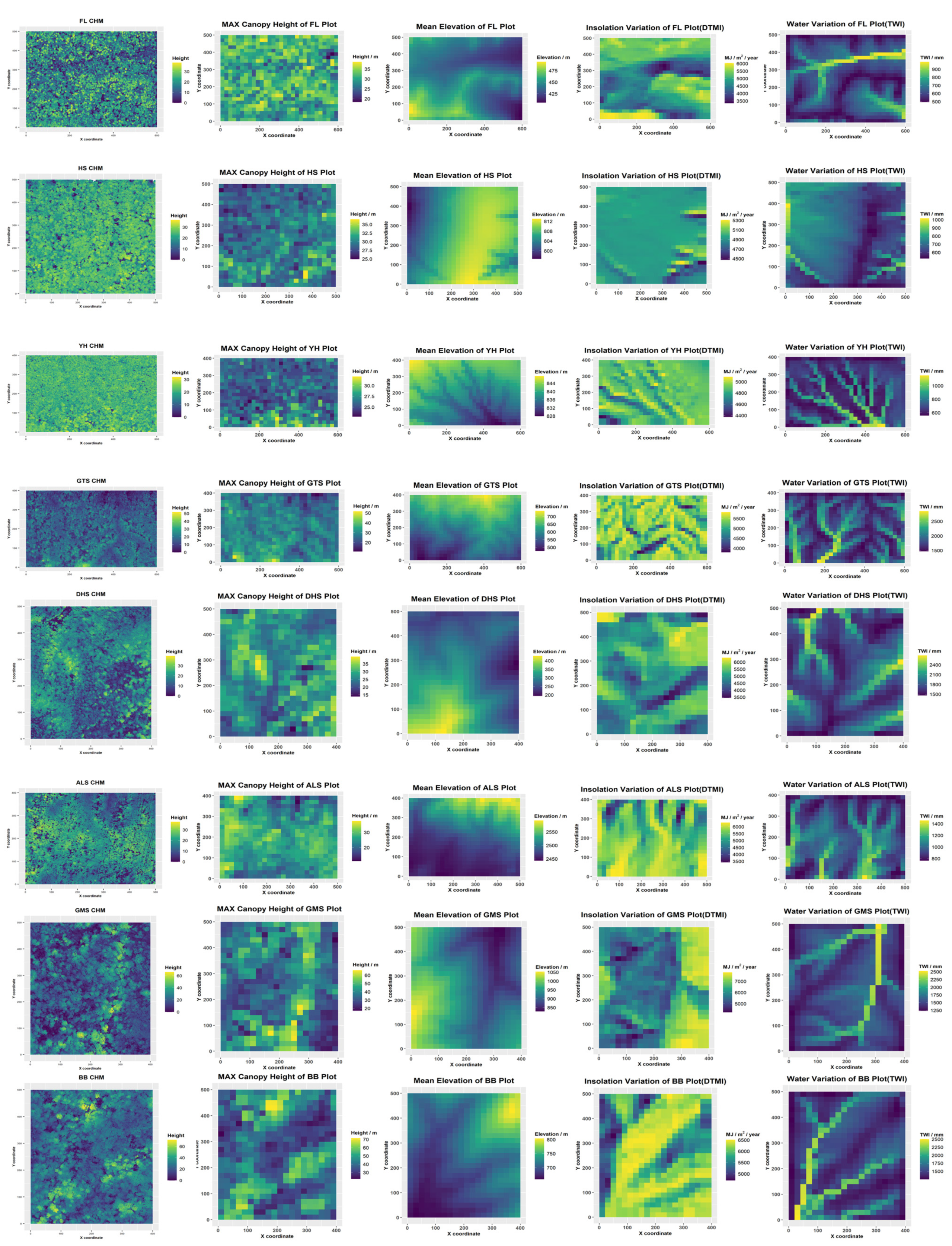
2.1. Study Sites and Forest Plots

Our research group is a member of the Chinese Forest Biodiversity Monitoring Network (CForBio, http://www.cncdiversitas.cn/zyxm/cforbio/js/, accessed on 1 December 2021). All plots were consistently set up following the protocol of the Center for Tropical Forest Science (ForestGeo-CTFS, https://forestgeo.si.edu/, accessed on 1 December 2021) [24]. We selected eight dynamic forest plots with an area of 20–30 ha in China (Figure 1). These forest plots covered a wide geographical range, from 48.133° N to 21.613° N, and included three temperate (FL, HS, and YH), three subtropical (GTS, DHS, and ALS), and two tropical (BB and GMS) forests. More detailed information about these forest plots can be found in

Table 1. Basic information of the eight plots in our study, including the abbreviation of the plot name, forest region, vegetation type, size, location, mean elevation and elevation difference in parentheses, mean annual precipitation (MAP) in millimeters (mm), and mean annual solar radiation (MAS) in MJ/m²/year.

Plot	Forest Region	Vegetation Type	Size	Location	Elevation	MAP	MAS
FL	Temperate	Primary broad-leaved Korean pine forest	30 ha (600 × 500 m)	48.133° N 129.200° E	419 (66)	629	4879.7
HS	Temperate	Primary broad-leaved Korean pine forest	25 ha (500 × 500 m)	42.383° N 128.089° E	801 (18)	680	4929.6
YH	Temperate	Secondary poplar-birch forest	24 ha (600 × 400 m)	42.372° N 128.005° E	832 (22)	701	4865.8
GTS	Subtropical	Evergreen broad-leaved forest	24 ha (600 × 400 m)	27.25° N 118.12° E	618 (277)	1844	5301.6
ALS	Subtropical	Mid-montane moist evergreen broad-leaved forest	20 ha (500 × 400 m)	24.53° N 101.03° E	2509 (157)	985	5515.1
DHS	Subtropical	Evergreen broad-leaved forest	20 ha (400 × 500 m)	23.167° N 112.591° E	350 (240)	1818	5022.9
GMS	Tropical	Tropical mountain rainforest	20 ha (500 × 400 m)	22.246° N 100.599° E	949 (237)	1574	6097.2
BB	Tropical	Tropical seasonal rainforest	20 ha (400 × 500 m)	21.613° N 101.580° E	735.5 (153)	1698	5967.9

and

Table A1. Soil types of 8 plots.

Plot Name	Soil Type	Point Cloud Density
FL	mountain brown forest soil	20 points/m2
HS	mountain dark brown forest soil	88 points/m2
YH	mountain dark brown forest soil	124 points/m2
GTS	krasnozem	20 points/m2
ALS	mountain yellow brown soil	57 points/m2
DHS	latosolic red soil	90 points/m2
GMS	Laterite	30 points/m2
BB	Laterite	22 points/m2

.

2.2. Near-Surface LiDAR Data

To make all the LiDAR data of all the forest plots comparable, we scanned the forests and obtained these data during the leaf-on season (FL, HS, and YH in July; GTS and DHS in October; BB, GMS, and ALS in March) in July 2017 and 2018. The point-cloud data were collected by LiAir-pro, a UAV-mountable LiDAR scanning system developed by Green Valley Inc. (Beijing, China, https://www.lidar360.com/, accessed on 1 December 2021). The point cloud density of each plot is in Table A1 in Appendix A. A digital terrain model (DTM) was gridded from ground point representations of the Earth’s surface, and a digital surface model (DSM) was gridded from high vegetation point representations of the actual canopy’s surface. A canopy height model (CHM) was constructed based on the difference between DEM and DSM and contained only the top canopy height information in each grid. We generated these three basic models, the basis for further analyses, at a 0.5 m resolution using Cloud Compare (http://www.cloudcompare.org/, accessed on 1 December 2021) and R. v3.5.3 software [25] with the R packages “lidR” and “raster”.

2.3. Parameter Extraction

In this study, we divided each forest plot into 20 × 20 m adjacent quadrats (grids) and then extracted the parameter from the LiDAR data of each quadrat. Hmax is each quadrat’s maximum canopy height calculated from the canopy height model. The topographic wetness index (TWI) and digital-terrain-model-derived insolation (DTMI) were calculated from the digital terrain model, which can represent the local variation in topographic-derived water and energy conditions [26]. TWI was defined as the natural logarithm of the upslope contributing area (a) and slope (b) as ln (a/tan b) [27,28]. The DTMI was defined as potential solar radiation on a sloping surface [29,30]. Topographically derived radiation varies with the geometry of the receiving surface, such as the surface gradient (slope) and orientation (aspect), as well as the position relative to the neighboring surfaces [29]. Meteorological data were obtained from the WorldClim website based on the geographical coordinates of each plot (http://worldclim.org/). The TWI and DTMI were extracted using the R packages “dynatopmodel” and “insol”, respectively.

To make different plots comparable, we first calculated the relative values of TWI and DTMI by dividing the quadrat-level value by the plot-level value. Then, we multiplied the plot-level mean annual precipitation (MAP) and solar radiation (MAS) by the relative value of TWI and DTMI in each quadrat, respectively. The formulas are as follows:

$$\mathrm{TWI}={\mathrm{TWI}}_{\mathrm{original}}÷{\mathrm{mean}\mathrm{TWI}}_{\mathrm{original}}\times \mathrm{plot}\mathrm{MAP}$$

(1)

$$\mathrm{DTMI}={\mathrm{DTMI}}_{\mathrm{original}}÷{\mathrm{mean}\mathrm{DTMI}}_{\mathrm{original}}\times \mathrm{plot}\mathrm{MAS}$$

(2)

We first coarsened the resolution of the DTM to 20 m via spatial averaging of 1 m LiDAR data, and two predictors were then calculated at this scale [22]; this ensured that the variable estimate did not have any extreme localized values, as often occurs when using a very high-resolution terrain model as the input source.

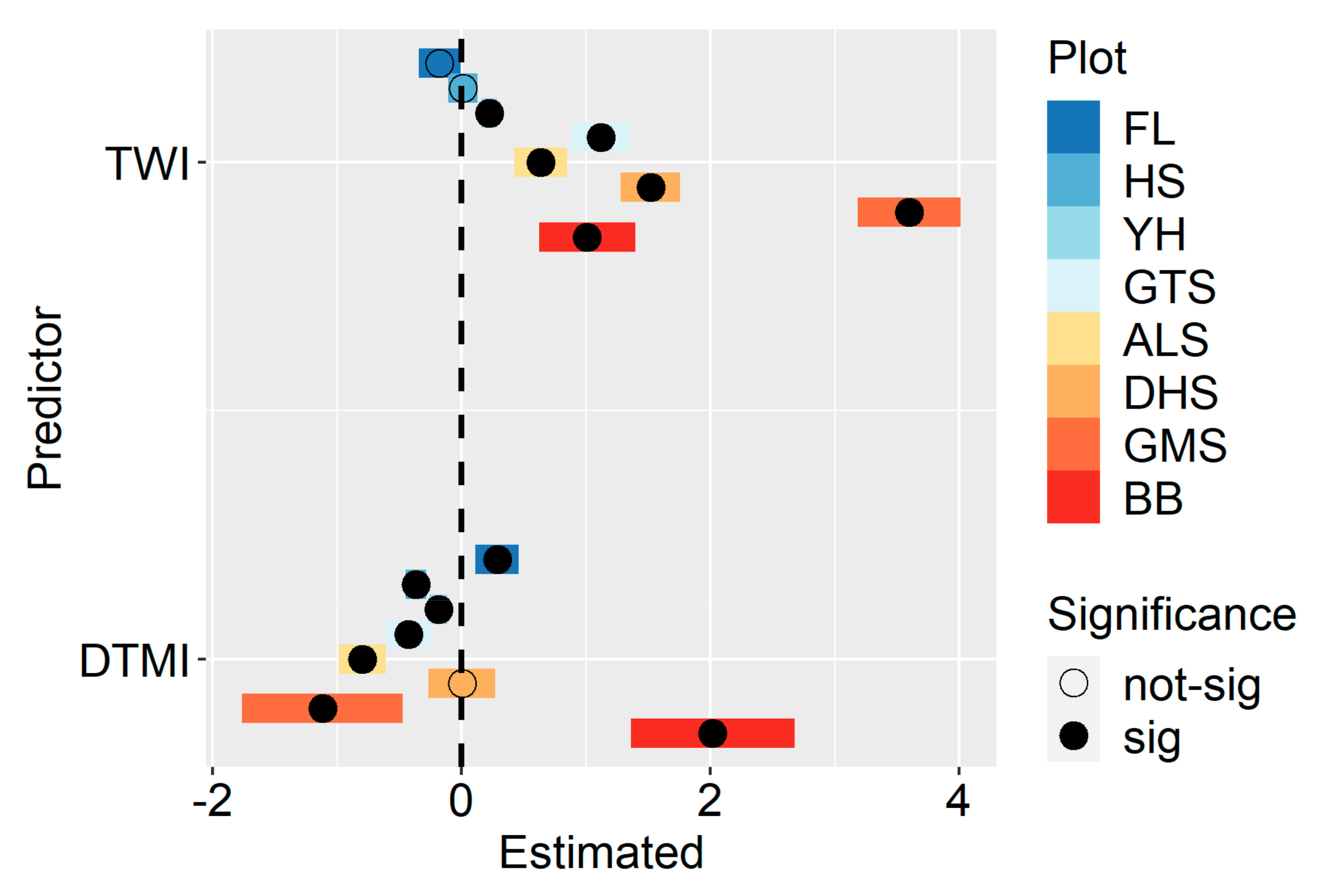
2.4. Statistical Analysis

We constructed a linear mixed model (LMM) to identify the effect of water and energy on Hmax. In LMM, we used TWI and DTMI as the fixed effects to predict the Hmax of 3667 quadrats from 8 plots. We built three kinds of LMMs to include “plot” as a random factor. The first model assumed that the “plot” only influenced the Hmax distinction among plots, which is the random intercept in the LMM. In the second model, we regarded the “plot” as the random slope, so it only affected the relationship between the explanatory variable and Hmax. In the third model, “plot” was used as a random slope and random intercept simultaneously. If the plot was a significant random factor in the relationship, it implied we should test the impact in each plot separately. The model was calculated with the R package “lmerTest”.

We next employed spatial simultaneous autoregressive error models (SARs) to explore the relationships between Hmax and the two predictors in each forest plot separately. This method allows the inclusion of residual spatial autocorrelation at a 20 m scale [31]. The spatial weight matrices were calculated with the nearest 4 adjacent quadrats in our model. The model was calculated with the R package “spDataLarge”.

Finally, we chose the LMG approach to evaluate the relative importance of two predictor variables (TWI and DTMI) in determining canopy height variation [15]. The relative importance of a predictor is the natural decomposition of the model R2, which differs from its estimated coefficients. To calculate the relative importance of variables in SAR, we first fit a SAR and then removed the spatial component of the fitted values by entering Hmax, excluding the spatial component as a new response variable in the R2 partitioning procedure [32]. The relative importance of the predictor variables was calculated using the R package “RELAIMPO”.

3. Results

The quadrat-level maximum canopy height ranged from 10 to 70 m across all forest plots (

Table 2. The information of eight plots related to Hmax in our study, including the mean Hmax, the standard deviation of Hmax, and the range of Hmax. The number of quadrats is the total number of 20 × 20 m quadrats in each forest plot. The number in parentheses represents the number of quadrats left after removing the boundary quadrats and the quadrats with the 5% lowest Hmax.

Plot	Mean Hmax	Hmax Range	Number of Quadrats
FL	30.87	18.44–38.57	750 (613)
HS	29.56	24.96–36.49	625 (509)
YH	26.14	22.81–32.11	600 (476)
GTS	28.54	11.05–51.69	600 (483)
ALS	25.65	11.15–37.52	500 (394)
DHS	26.73	13.97–39.74	500 (400)
GMS	37.70	17.27–66.03	500 (399)
BB	41.9	22.24–71.51	500 (393)

). The GMS and BB plots had the greatest quadrat maximum canopy height of around 70 m, while the mean Hmax of the eight plots was approximately 40 m. The quadrat canopy height of the HS and YH plots was highly centralized, compared with that of the six other plots. More information such as CHM and DEM of each plot is in Figure A1.

The LMM included plot as the random intercept and the slope was the best model, with the lowest AIC and highest R-square value of 0.633 (

Table 3. The result of the linear mixed model (LMM) with three types of random effects. * indicates the significance of the models and predictors. *** means p-value < 0.001, * means p-value < 0.05.

LMM Type	R2	AIC	TWI	DTMI
Random intercept ***	0.591	22,128.89	6.19 ***	−0.06
Random slope model ***	0.611	21,968.44	3.72	−0.22
Random intercept and slope ***	0.633	21,787.15	4.21 *	−0.35

). TWI was highly significantly positively related to all quadrat maximum canopy heights (coefficient = 4.21, p < 0.01), and the DTMI was weakly and non-significantly negatively related to the Hmax (coefficient = −0.35, p > 0.1).

We found that TWI showed a significant, positive influence except in the FL and HS plots. DTMI had a significant influence except in the DHS plot. The effect of DTMI was positive in the FL and BB plots but negative in the other five plots. Interestingly, we found that the effect of TWI changed from a non-significant, negative effect to a significant, positive effect when changing locations from temperate to tropical forests. The effect of DTMI showed a similar directional change pattern from positive to negative when the forest types changed from temperate to tropical forests, except in the BB forest plots (Figure 2). The detailed information is in

Table A2. Results for the fitted spatial simultaneous autoregressive error models (SARs).

Plot	Predictor	p Value	Mean	SD	Min	Max
FL	TWI	0.29	−0.18	0.17	−0.35	−0.008
FL	DEML	.	0.29	0.17	0.11	0.46
HS	TWI	0.93	0.01	0.12	−0.11	0.13
HS	DEML	***	−0.37	0.08	−0.45	−0.28
YH	TWI	***	0.22	0.07	0.16	0.29
YH	DEML	*	−0.19	0.07	−0.26	−0.11
GTS	TWI	***	1.12	0.23	0.89	1.35
GTS	DEML	*	−0.42	0.18	−0.60	−0.24
ALS	TWI	**	0.64	0.21	0.43	0.85
ALS	DEML	***	−0.80	0.19	−0.99	−0.61
DHS	TWI	***	1.52	0.24	1.28	1.76
DHS	DEML	0.99	0.001	0.27	−0.26	0.27
GMS	TWI	***	3.60	0.41	3.18	4.01
GMS	DEML	.	−1.12	0.65	−1.76	−0.47
BB	TWI	**	1.01	0.39	0.62	1.40
BB	DEML	**	2.02	0.66	1.36	2.68

‘.’ represents a p value between 0.1 and 0.05, ‘*’ represents a p value between 0.05 and 0.01, ‘**’ represents a p value between 0.01 and 0.001, and ‘***’ represents a p value less than 0.001.

.

We found that DTMI had higher importance in temperate forests, while TWI had a stronger explanatory power in subtropical and tropical forests (Figure 3). The DTMI accounted for more than 90% of the total variation in the two temperate forest plots (i.e., FL and HS plots), while DTMI explained less than 10% of the variation in the subtropical and tropical forest plots (except for ALS). Unexpectedly, we found TWI was slightly more important than DTMI in the YH plot, which is a typical secondary temperate forest. The detailed information is in

Table A3. Relative importance results of the spatial simultaneous autoregressive error models (SARs).

Plot Name	TWI (%)	DTMI (%)
FL	5.67	94.33
HS	2.21	97.79
YH	59.82	40.18
GTS	83.65	16.35
ALS	53.30	46.70
DHS	97.08	2.92
GMS	95.52	4.48
BB	84.18	15.82

.

4. Discussion

Understanding the patterns and determinants of forest canopy height variation can provide critical insights into the drivers of ecosystem functions [33]. Despite an extensive body of research on canopy height variation, few studies have focused on the patterns and determinants of canopy height variation at the local scale. In this study, based on near-surface LiDAR data from eight large permanent forest plots in China, we accurately measured canopy height variation at the local scale and quantified the relative contributions of energy and water limitations to canopy height variation from temperate to tropical forests.

In this study, we found that TWI, rather than DTMI, was the major driver of maximum canopy height variation when we combined all plots, supporting the hydraulic limitation hypothesis. Previous studies demonstrated that canopy height variation is mainly affected by water limitation at both global and regional scales [19,20,34]. Our results further highlighted the dominant role of water availability in controlling forest canopy height at the local scale. The positive relationship between TWI and Hmax suggested that higher water availability can increase the maximum canopy height. Higher maximum canopy height and vertical heterogeneity could lead to greater use of niche space for light and provide multidimensional space that can be occupied by different species [33]. Therefore, our results suggest that ensuring the water availability of plants, especially large trees, is an important prerequisite for effectively maintaining biodiversity at the local scale. The altitude of the ALS plot is 2509 m, which causes the water vapor in the cloud to act as an important supplement of water, thus alleviating the effect of water limitation on the canopy height of the ALS plot. In the context of global climate change, more frequent and devastating droughts have reduced the soil water content, streamflow, and groundwater recharge [35,36]. Further studies are required to investigate how drought influences biodiversity maintenance by altering the complexity of the canopy structure.

When we focused on individual plots, we found that the TWI had limited influence on the canopy height variation in the temperate forest plots. This is because trees grow mainly in the summer when precipitation is high in the temperate forests of East Asia. The abundant water supplies contribute to the weak relationship between large trees and water availability. We also found that the positive effect of TWI increased significantly from temperate to tropical forests, suggesting that the spatial distribution of large trees is more related to the local water variability in subtropical and tropical forests. This result is similar to that found in previous studies, i.e., that water availability can determine plant species distribution in tropical forests [37,38]. Species with different heights can develop corresponding adaptive strategies to water availability through hydraulic regulation [39]. Therefore, trees growing in areas with higher water availability can invest more resources into height growth rather than hydraulic conductivity [40]. Furthermore, two studies have found that species co-existing within a community often have specific habitat preferences [41,42]. Our study supported this view by identifying the relationship between tree height and water availability; that is, species with greater height tend to grow in areas with high water availability.

Although the relationship between DTMI and canopy height variation was non-significant when we combined all plots, we found that DTMI had a significant influence on canopy height variation in most individual forest plots. This result highlights the necessity of local-scale analysis for our understanding of canopy height variation. Most importantly, we found that DTMI had higher importance in temperate forests than in subtropical and tropical forests. This finding supports the idea that energy is an important factor regulating canopy height variation in high-latitude forests because of the low temperature and high heterogeneity of solar radiation [26,43]. However, different from previous results supporting the energy limitation hypothesis, our study demonstrated that the effect of energy on canopy height variation can be both positive and negative in temperate forests. The first possible reason for this finding may stem from the geographical characteristics of temperate forests. Temperate forests are located near the middle of a full latitudinal gradient from tropical forests to boreal forests and contain flora from temperate, subtropical, and subarctic zones. Global analysis suggests that the drivers of canopy height variation change from energy to water when the forest type shifts from boreal to tropical [15]. Therefore, temperate forests are in a transition zone from energy-limited to water-limited geography, and the complex flora composition makes it possible for forest canopy heights to respond differently to energy and water limitations. The second possible explanation is the local habitat heterogeneity. We found a large elevation difference in the FL plot. Due to the undulating terrain, the energy at lower elevations is usually lower than that at higher elevations. As a result, the vertical growth of plants can benefit from higher energy availability when growing in higher elevation areas, resulting in a positive relationship between canopy height and energy availability. In contrast, the HS plot had a relatively flat terrain and a relatively uniform and low energy distribution. Thus, plants grown in relatively energy-poor areas can mitigate the adverse effects of the energy deficit by increasing their height, and then their canopy heights are greater than those grown in energy-sufficient areas. This may explain why we observed an inverse relationship between canopy height and energy availability.

5. Conclusions

In this study, we explored the role of the “water limitation hypothesis” and the “energy limitation hypothesis” in explaining canopy height variation of forest communities at the local scale. Our study showed that energy explained more variance of canopy height in temperate forest while hydraulic limitation explained more variance of canopy height in subtropical and tropical forests. Especially, the positive effect of available water on Hmax increased from temperate to subtropical and tropical forests. The directional change in drivers implied differences in the ability of diverse forests to tolerate future changes in climate or anthropogenic disturbance regimes. These results shed light on the potential ecological mechanisms driving ecosystem functions and could potentially benefit biodiversity conservation.

References

1. Ozanne, C.M.P.; Anhuf, D.; Boulter, S.L.; Keller, M.; Kitching, R.L.; Körner, C.; Meinzer, F.C.; Mitchell, A.W.; Nakashizuka, T.; Dias, P.L.S.; et al. Biodiversity Meets the Atmosphere: A Global View of Forest Canopies. Science 2003, 301, 183–186. [Google Scholar] [CrossRef] [PubMed] [Green Version]
2. Fotis, A.T.; Morin, T.H.; Fahey, R.T.; Hardiman, B.S.; Bohrer, G.; Curtis, P.S. Forest Structure in Space and Time: Biotic and Abiotic Determinants of Canopy Complexity and Their Effects on Net Primary Productivity. Agric. For. Meteorol. 2018, 250–251, 181–191. [Google Scholar] [CrossRef]
3. Lefsky, M.A.; Harding, D.J.; Keller, M.; Cohen, W.B.; Carabajal, C.C.; Del Bom Espirito-Santo, F.; Hunter, M.O.; de Oliveira, R., Jr. Estimates of Forest Canopy Height and Aboveground Biomass Using ICESat. Geophys. Res. Lett. 2005, 32, L22S02. [Google Scholar] [CrossRef] [Green Version]
4. Simard, M.; Fatoyinbo, L.; Smetanka, C.; Rivera-Monroy, V.H.; Castañeda-Moya, E.; Thomas, N.; Van der Stocken, T. Mangrove Canopy Height Globally Related to Precipitation, Temperature and Cyclone Frequency. Nat. Geosci. 2019, 12, 40–45. [Google Scholar] [CrossRef]
5. Lefsky, M.A. A Global Forest Canopy Height Map from the Moderate Resolution Imaging Spectroradiometer and the Geoscience Laser Altimeter System. Geophys. Res. Lett. 2010, 37, L15401. [Google Scholar] [CrossRef] [Green Version]
6. Simard, M.; Pinto, N.; Fisher, J.B.; Baccini, A. Mapping Forest Canopy Height Globally with Spaceborne Lidar. J. Geophys. Res. Biogeosci. 2011, 116, G04021. [Google Scholar] [CrossRef] [Green Version]
7. Zimmermann, U.; Schneider, H.; Wegner, L.H.; Haase, A. Water Ascent in Tall Trees: Does Evolution of Land Plants Rely on a Highly Metastable State? New Phytol. 2004, 162, 575–615. [Google Scholar] [CrossRef]
8. Cramer, M. Unravelling the Limits to Tree Height: A Major Role for Water and Nutrient Trade-Offs. Oecologia 2011, 169, 61–72. [Google Scholar] [CrossRef]
9. Canny, M.J. A New Theory for the Ascent of Sap—Cohesion Supported by Tissue Pressure. Ann. Bot. 1995, 75, 343–357. [Google Scholar] [CrossRef]
10. Binkley, D.; Stape, J.L.; Ryan, M.G.; Barnard, H.R.; Fownes, J. Age-Related Decline in Forest Ecosystem Growth: An Individual-Tree, Stand-Structure Hypothesis. Ecosystems 2002, 5, 58–67. [Google Scholar] [CrossRef]
11. Rust, S.; Roloff, A. Reduced Photosynthesis in Old Oak (Quercus Robur): The Impact of Crown and Hydraulic Architecture. Tree Physiol. 2002, 22, 597–601. [Google Scholar] [CrossRef] [PubMed]
12. Stephenson, N. Actual Evapotranspiration and Deficit: Biologically Meaningful Correlates of Vegetation Distribution across Spatial Scales. J. Biogeogr. 1998, 25, 855–870. [Google Scholar] [CrossRef]
13. Ryan, M.G.; Yoder, B.J. Hydraulic Limits to Tree Height and Tree Growth. BioScience 1997, 47, 235–242. [Google Scholar] [CrossRef] [Green Version]
14. Larjavaara, M. The World’s Tallest Trees Grow in Thermally Similar Climates. New Phytol. 2014, 202, 344–349. [Google Scholar] [CrossRef] [PubMed]
15. Zhang, J.; Nielsen, S.E.; Mao, L.; Chen, S.; Svenning, J.-C. Regional and Historical Factors Supplement Current Climate in Shaping Global Forest Canopy Height. J. Ecol. 2016, 104, 469–478. [Google Scholar] [CrossRef] [Green Version]
16. Koch, G.W.; Sillett, S.C.; Jennings, G.M.; Davis, S.D. The Limits to Tree Height. Nature 2004, 428, 851–854. [Google Scholar] [CrossRef]
17. Reich, P.B.; Luo, Y.; Bradford, J.B.; Poorter, H.; Perry, C.H.; Oleksyn, J. Temperature Drives Global Patterns in Forest Biomass Distribution in Leaves, Stems, and Roots. Proc. Natl. Acad. Sci. USA 2014, 111, 13721–13726. [Google Scholar] [CrossRef] [Green Version]
18. Moles, A.T.; Warton, D.I.; Warman, L.; Swenson, N.G.; Laffan, S.W.; Zanne, A.E.; Pitman, A.; Hemmings, F.A.; Leishman, M.R. Global Patterns in Plant Height. J. Ecol. 2009, 97, 923–932. [Google Scholar] [CrossRef]
19. Klein, T.; Randin, C.; Körner, C. Water Availability Predicts Forest Canopy Height at the Global Scale. Ecol. Lett. 2015, 18, 1311–1320. [Google Scholar] [CrossRef]
20. Tao, S.; Guo, Q.; Li, C.; Wang, Z.; Fang, J. Global Patterns and Determinants of Forest Canopy Height. Ecology 2016, 97, 3265–3270. [Google Scholar] [CrossRef]
21. Baldeck, C.A.; Harms, K.E.; Yavitt, J.B.; John, R.; Turner, B.L.; Valencia, R.; Navarrete, H.; Davies, S.J.; Chuyong, G.B.; Kenfack, D.; et al. Soil Resources and Topography Shape Local Tree Community Structure in Tropical Forests. Proc. R. Soc. B Biol. Sci. 2013, 280, 20122532. [Google Scholar] [CrossRef] [PubMed]
22. Jucker, T.; Bongalov, B.; Burslem, D.F.R.P.; Nilus, R.; Dalponte, M.; Lewis, S.L.; Phillips, O.L.; Qie, L.; Coomes, D.A. Topography Shapes the Structure, Composition and Function of Tropical Forest Landscapes. Ecol. Lett. 2018, 21, 989–1000. [Google Scholar] [CrossRef] [PubMed]
23. Fortunel, C.; Lasky, J.R.; Uriarte, M.; Valencia, R.; Wright, S.J.; Garwood, N.C.; Kraft, N.J.B. Topography and Neighborhood Crowding Can Interact to Shape Species Growth and Distribution in a Diverse Amazonian Forest. Ecology 2018, 99, 2272–2283. [Google Scholar] [CrossRef] [PubMed]
24. Feng, G.; Mi, X.; Yan, H.; Li, F.Y.; Svenning, J.-C.; Ma, K. CForBio: A Network Monitoring Chinese Forest Biodiversity. Sci. Bull. 2016, 61, 1163–1170. [Google Scholar] [CrossRef] [Green Version]
25. R Core Team. R: A Language and Environment for Statistical Computing; R Foundation for Statistical Computing: Vienna, Austria, 2013. [Google Scholar]
26. Fricker, G.A.; Synes, N.W.; Serra-Diaz, J.M.; North, M.P.; Davis, F.W.; Franklin, J. More than Climate? Predictors of Tree Canopy Height Vary with Scale in Complex Terrain, Sierra Nevada, CA (USA). For. Ecol. Manag. 2019, 434, 142–153. [Google Scholar] [CrossRef] [Green Version]
27. Sørensen, R.; Zinko, U.; Seibert, J. On the Calculation of the Topographic Wetness Index: Evaluation of Different Methods Based on Field Observations. Hydrol. Earth Syst. Sci. Discuss. 2006, 10, 101–112. [Google Scholar] [CrossRef] [Green Version]
28. Grabs, T.; Seibert, J.; Bishop, K.; Laudon, H. Modeling Spatial Patterns of Saturated Areas: A Comparison of the Topographic Wetness Index and a Dynamic Distributed Model. J. Hydrol. 2009, 373, 15–23. [Google Scholar] [CrossRef] [Green Version]
29. Kumar, L.; Skidmore, A.K.; Knowles, E. Modelling Topographic Variation in Solar Radiation in a GIS Environment. Int. J. Geogr. Inf. Sci. 1997, 11, 475–497. [Google Scholar] [CrossRef]
30. Fu, P.; Rich, P.M. A Geometric Solar Radiation Model with Applications in Agriculture and Forestry. Comput. Electron. Agric. 2002, 37, 25–35. [Google Scholar] [CrossRef]
31. Kissling, W.D.; Carl, G. Spatial Autocorrelation and the Selection of Simultaneous Autoregressive Models. Glob. Ecol Biogeogr. 2007, 17, 59–71. [Google Scholar] [CrossRef]
32. Belmaker, J.; Jetz, W. Cross-Scale Variation in Species Richness-Environment Associations: Richness-Environment Scaling. Glob. Ecol. Biogeogr. 2011, 20, 464–474. [Google Scholar] [CrossRef]
33. Pan, Y.; Birdsey, R.A.; Phillips, O.L.; Jackson, R.B. The Structure, Distribution, and Biomass of the World’s Forests. Annu. Rev. Ecol. Evol. Syst. 2013, 44, 593–622. [Google Scholar] [CrossRef] [Green Version]
34. Givnish, T.J.; Wong, S.C.; Stuart-Williams, H.; Holloway-Phillips, M.; Farquhar, G.D. Determinants of Maximum Tree Height in Eucalyptus Species along a Rainfall Gradient in Victoria, Australia. Ecology 2014, 95, 2991–3007. [Google Scholar] [CrossRef] [Green Version]
35. Cai, W.; Cowan, T. Dynamics of Late Autumn Rainfall Reduction over Southeastern Australia. Geophys. Res. Lett. 2008, 35, L09708. [Google Scholar] [CrossRef]
36. Vicente-Serrano, S.M.; Lopez-Moreno, J.-I.; Beguería, S.; Lorenzo-Lacruz, J.; Sanchez-Lorenzo, A.; García-Ruiz, J.M.; Azorin-Molina, C.; Morán-Tejeda, E.; Revuelto, J.; Trigo, R.; et al. Evidence of Increasing Drought Severity Caused by Temperature Rise in Southern Europe. Environ. Res. Lett. 2014, 9, 044001. [Google Scholar] [CrossRef]
37. Engelbrecht, B.M.J.; Comita, L.S.; Condit, R.; Kursar, T.A.; Tyree, M.T.; Turner, B.L.; Hubbell, S.P. Drought Sensitivity Shapes Species Distribution Patterns in Tropical Forests. Nature 2007, 447, 80–82. [Google Scholar] [CrossRef] [PubMed]
38. Poorter, L.; Markesteijn, L. Seedling Traits Determine Drought Tolerance of Tropical Tree Species. Biotropica 2008, 40, 321–331. [Google Scholar] [CrossRef]
39. Liu, H.; Gleason, S.M.; Hao, G.; Hua, L.; He, P.; Goldstein, G.; Ye, Q. Hydraulic Traits Are Coordinated with Maximum Plant Height at the Global Scale. Sci. Adv. 2019, 5, eaav1332. [Google Scholar] [CrossRef] [Green Version]
40. Comita, L.S.; Condit, R.; Hubbell, S.P. Developmental Changes in Habitat Associations of Tropical Trees. J. Ecol. 2007, 95, 482–492. [Google Scholar] [CrossRef]
41. Webb, C.O.; Peart, D.R. Habitat Associations of Trees and Seedlings in a Bornean Rain Forest. J. Ecol. 2000, 88, 464–478. [Google Scholar] [CrossRef]
42. Allié, E.; Pélissier, R.; Engel, J.; Petronelli, P.; Freycon, V.; Deblauwe, V.; Soucémarianadin, L.; Weigel, J.; Baraloto, C. Pervasive Local-Scale Tree-Soil Habitat Association in a Tropical Forest Community. PLoS ONE 2015, 10, e0141488. [Google Scholar] [CrossRef] [PubMed]
43. Ameztegui, A.; Rodrigues, M.; Gelabert, P.J.; Lavaquiol, B.; Coll, L. Maximum Height of Mountain Forests Abruptly Decreases above an Elevation Breakpoint. GIScience Remote Sens. 2021, 58, 442–454. [Google Scholar] [CrossRef]
Figure 1. Locations of the 8 forest plots in China. Each solid point indicates a plot location, and the color represents the elevation in China.
Forests 13 00639 g001
Figure 2. Results of the spatial simultaneous autoregressive error models (SARs). Colors represent forest plots from tropical (red) to temperate (blue) latitudes. The solid circle in the colored bar indicates significance at the 0.1 level. The black dotted line indicates no relationship. The colored bar on the left of the dotted line indicates a negative effect, and those on the right indicate a positive result. The X-axis is the estimated coefficient.
Forests 13 00639 g002
Figure 3. Result of the relative importance of two predictors (TWI and DTMI) in spatial simultaneous autoregressive error models (SARs). TWI is the blue part, and the red part represents the relative importance of DTMI in each plot. Results are arranged in descending latitude from left to right.
Forests 13 00639 g003