Article

Species Diversity, Biomass and Carbon Stock Assessment of Kanhlyashay Natural Mangrove Forest

1
School of Forestry, Beijing Forestry University, Tsinghua East Road, Haidian District, Beijing 100083, China
2
School of Ecology and Nature Conservation, Beijing Forestry University, Tsinghua East Road, Haidian District, Beijing 100083, China
*
Author to whom correspondence should be addressed.
Forests 2022, 13(7), 1013; https://doi.org/10.3390/f13071013
Submission received: 9 May 2022 / Revised: 10 June 2022 / Accepted: 15 June 2022 / Published: 28 June 2022

Abstract

:
Mangrove ecosystems sequester and store large amounts of carbon in both biomass and soil. In this study, species diversity, the above and below-ground biomass as well as carbon stock by the mangroves in Kanhlyashay natural mangrove forest were estimated. Six true mangrove species from four families were recorded in the sample plots of the study area. Among them, Avicennia officinalis L. from the Acanthaceae family was the abundance of species with an importance value of 218.69%. Shannon–Wiener’s diversity index value (H′ = 0.71) of the mangrove community was very low compared to other natural mangrove forests since the mangrove stands in the study site possessed a low number of mangrove species and were dominated by a few species. Estimated mean biomass was 335.55 ± 181.41 Mg ha−1 (AGB = 241.37 ± 132.73 Mg ha−1, BGB = 94.17 ± 48.73 Mg ha−1). The mean overall C-stock of the mangrove stand was 150.25 ± 81.35 Mg C ha−1 and is equivalent to 551.10 ± 298.64 Mg CO2 eq. The role of forests in climate change is two-fold as a cause and a solution for greenhouse gas emissions. The result of the study demonstrated that the mangroves in Letkhutkon village have high carbon storage potential, therefore it is necessary to be sustainably managed to maintain and increase carbon storage. Climate change mitigation may be achieved not only by reducing the carbon emission levels but also by maintaining the mangrove ecosystem services as carbon sinks and sequestration.

1. Introduction

Mangrove forests are one of the most productive and diverse ecosystems in the world and provide significant ecological, economic, and social benefits [1]. The ecological benefits supported by the mangrove forests are bio-protection from littoral erosion [2,3], shoreline stabilizations, reducing the devastating impact of hurricanes, waves, and tsunamis, and protection from cyclones [3,4]. Additionally, mangrove ecosystems have a high carbon sequestration capacity, which is reflected in high aboveground biomass, high net primary production (NPP), the low decomposition rate of mangrove sediments, and belowground to aboveground biomass rations [5,6,7,8]. Mangrove forests have a critical role in climate change mitigation because they are able to absorb and store 3–5 times more carbon than other upland forests, mainly in soil [5]. Despite accounting <1% of the world’s tropical forest area [9], mangroves account for 3–4% of global carbon sequestration by the total tropical forest area [10,11] and contribute 10–15% to the carbon sequestered by the world’s ocean [9]. Globally, the average carbon stock of the mangrove ecosystem is 1023 Mg ha−1 [5]; consequently, mangrove ecosystems are now being recognized for their pivotal role in global climate change mitigation. Concerning the characteristics of high carbon reservation and huge ecological benefits, mangrove ecosystems are eligible for inclusion in the United Nation’s Reduce Emissions from Deforestation and Forest Degradation and to Enhance Carbon Stocks (REDD+) strategies [12] as well as the payments for ecosystem services (PES) [13] initiatives that are emerging in many countries. On the other side, the deforestation rate of mangrove forests is still higher than inland terrestrial forests. Globally, it is estimated that mangrove forests have been lost with an annual average rate of 0.16% to 0.39% [14] and pose a significant risk to carbon emission as a consequence of mangrove deforestation.
Mangrove forests in Myanmar grow along the 2832 km-long coastlines, oriented along the Bay of Bengal and the Andaman Sea [15]. The total area of mangroves in Myanmar reaches 3.3% of the total area of mangroves of the world [15,16], and mangrove forest types can be divided into Delta Mangrove and Coastal Mangrove [17]. Mangrove ecosystems provide important services such as ecological, economic, and environmental benefits to local people; however, mangrove coverage in Myanmar has decreased by more than half of the total mangrove area over the past three decades. Myanmar is regarded as the current mangrove deforestation hotspot globally [18] with the highest annual rates (~1%) of mangrove deforestation and third-highest potential annual CO2 emissions (784 kg CO2eyr−1) [19]. The biggest drivers of mangrove deforestation in Myanmar are over-exploitation, illegal felling, agricultural expansion, and conversion to fish and shrimp ponds [20]. The inventory of carbon stocks in mangrove ecosystems is limited, and only a few studies have quantified the carbon stocks of these ecosystems in Myanmar.
Forest biomass is regarded as an important variable in quantifying the role of forests in the carbon cycle [21]; thus, the estimation of biomass is crucial for studying the carbon cycle of the forest ecosystem. Allometric models are widely applied for biomass estimation of mangrove forests [22] and allometric equations for biomass estimation are developed by applying physical parameters of the tree, such as height, diameter at breast height, basal area, density, and their combination. The objectives of the present study were to (i) estimate the species diversity of mangrove stands, (ii) evaluate the potential of biomass and carbon stock, and (iii) explore the relationships of stand-level carbon stock to stand structural variables such as mean diameter, mean height, basal area and their combination.

2. Materials and Methods

2.1. Description of Study Site

The research was carried out in the Kanhlyashay natural mangrove forests located at the estimated coordinates 16°21′26.93″ N and 96°13′02.37″ E. The mangrove stands naturally reappeared on the mudflat after the Cyclone Nargis wreaked havoc in 2008. The abundant growth of mangroves lies around 1–8 m above the current level of the sea and covers approximately 197 ha (487 acres) along the banks of the sea; then, the mangroves serve as a natural barrier against natural disasters such as sea-level rise, storm surges, and floods and help minimize the damage done to property and life in the Letkhutkon village located in the Kungyangon township of Yangon Division. The Kanhlyashay natural mangrove forest has planned to designate as a protected public forest by the Forest Department, Ministry of Natural Resources and Environmental Conservation, Myanmar. The soil formation in the study site has been underlain by the intertidal mudflats that are essential habitats for many fishes as nurseries and feeding grounds. Most of the local communities in the Letkhutkon village depend on small-scale marine fisheries for their livelihood; this area has an average precipitation of 2375 mm, with an average temperature of 26.8 °C and a tropical monsoon climate [23]. The study site was selected based on accessibility and safety in going to and from the natural mangrove stands. Additionally, this study is the first comprehensive forest inventory in the Kanhlyashay natural mangrove forests. The natural mangrove formation has been dominated by Avicennia officinalis L. in association with Sonneratia apetala Buch. Ham., S. caseolaris (L.) Engl., and Aegiceras corniculatum (L.) Blanco; then, Avicennia alba Blume and Bruguiera sexangula (Lour.) Poir. are rarely observed in the mangrove stand.
The fieldwork was performed from June to July 2021 during the rainy season. Letkhokkon village near the Andaman Sea has equal lengths of dry and rainy seasons. The wet season is oppressive and overcast, the dry season is muggy and partly cloudy, and it is hot year-round. Throughout the year, the temperature typically varies from 19 °C to 36 °C and is rarely below 17 °C or above 39 °C. The hottest month of the year is April with an average maximum temperature of 37 °C and the coldest month is January with an average low of 19 °C and a high of 32 °C. A map of the research stations was presented in Figure 1.

2.2. Data Collection

A total of 25 sampling plots of 400 m2 were established through a non-destructive quadrat sampling technique to determine the species composition, biomass, and carbon stock in the study area. The total sampling area covered was 0.5% (1 ha) of the total area. A global positioning system (GPS) was used to mark the spatial location of each sampling pot. Within each sampling plot, all trees with a diameter at breast height (dbh) of ≥5 cm were measured, identified, and counted. A diameter tape was used to measure the dbh; total tree heights were estimated using Suunto Clinometer. The dbh of Bruguiera and Rhizophora species were determined by measuring the trunk diameter at 30 cm above the buttress and above the highest prop root, respectively, whereas the dbh of the rest was measured at 130 cm above ground [24]. The distribution of stand density, species composition, biomass, and carbon stock per plot of the natural mangrove stand in LetKhutKon Village was described in Table 1.

2.3. Species Composition and Diversity

Species composition and diversity were calculated based on the forest inventory data. Species composition is the number of different species in the study area; it can be described in terms of relative density (RD), relative frequency (RF), and relative basal area (RBA). The importance value index (IVI) provides an overview of the influence or role of a type of mangrove species in the community. Importance values of a species range from 0–300%, and tree species having an IVI of more than 10% were considered dominant tree species in this study. The formula used to calculate RD, RBA, RF, and IVI were listed below.
RD = (Number of individuals of a species/Total number of individuals of all species) × 100
RBA = (combined BA of a species/total BA of all species) × 100
RF = (frequency of a species/sum of all frequencies) × 100
IVI = RD + RBA + RF
The basal area was calculated as
BA / Tree   ( m 2 ) = π   × ( DBH ) 2 × 0.0001 4
where π = a constant (3.146); DBH = diameter at breast height (cm), 0.0001 is a constant used to convert the measured centimetre square into meter square.
Total   Stand   Basal   Area   ( m 2 / ha ) = Sum   of   basal   area   for   each   tree 0.04 = Sum   of   basal   area   ×   25
where 0.04 is plot size in hectare and 25 is a constant used to extrapolate the measurement of the basal area from per plot (m2/plot) to per hectare (m2/ha).
The Species Diversity index, determined in this study using the Shannon–Wiener’s Index [25], indicated a quantitative description of mangrove habitat in terms of species distribution and evenness; this species diversity index was used in several studies [26,27,28] and was calculated using the following form:
H′ = −∑ PilnPi
where:
  • H′ = the value of the Shannon–Wiener diversity index
  • Pi = the proportion of ith species individuals to total species individuals
  • ln = the natural logarithm of Pi
Evenness Index, E = H′/ln(S)
where, S = Number of species in the study area

Aboveground and Belowground Biomass Estimation and Carbon Stocks

Inside each plot, all mangrove trees ≥ 5 cm in diameter were identified according to W. Giesen et al. [29] and measured the trunk diameters (cm) and total height (m) for estimating above and below-ground biomass. Tree measurements, including diameter at breast height (dbh) and height (H) in sample plots, were converted into tree biomass by using an allometric equation (tree biomass equation) and then into carbon stock. Here, allometric equations adapted from Komiyama et al. [30] were used to estimate AGB and BGB as shown in (Equations (9) and (10)). The reason for choosing these allometric equations was they utilized mangroves of Southeast Asia as samples when developing the equations, and were favoured by many researchers as they didn’t require tree height data.
The mean value of wood density (ρ) of each species was obtained from the Global Wood Density Database [31] by using the getWoodDensity function from the “BIOMASS” package in R program. Then, total aboveground and belowground biomass production in the plots were obtained by summing the biomass of all the standing trees and the biomass of each sample plot had been converted to stand-level biomass (Mg ha−1). Then, carbon stock of aboveground and belowground biomass showed in mega-grams per hectare (Mg C ha−1).
AGB = 0.251ρ D2.46
BGB = 0.199 ρ0.899 D2.22
where:
  • AGB (kg) = aboveground biomass estimates in kg per tree
  • BGB (kg) = belowground biomass estimate in kg per tree
  • D = diameter at breast height (dbh) in cm
  • ρ = wood density in g cm−3
The AGB and BGB were converted to above and below-ground carbon stock by multiplying 0.47 and 0.39 as a conversion factor [32,33,34,35,36] using the equations below:
Aboveground carbon stock = AGB × 0.47
Belowground carbon stock = BGB × 0.39

2.4. Statistical Analyses and Modelling Work

Regression analysis was used to establish allometric relationships of stand-level aboveground biomass carbon stock (Mg C ha−1) with mean DBH (cm), mean height (m), and stand basal area (m2 ha−1). In forest biomass studies, the error variances for the allometric non-linear equations based on arithmetical units of measurement were not constant over all observations (heteroscedasticity) in most cases [37,38]. Using log-transformed data for linear regressions was the most commonly used method for the estimation of parameters in non-linear models to eliminate the effects of heteroscedasticity [38]. To minimize the systematic bias, a correction factor (CF) was calculated for each model [39]. The stand-level aboveground carbon stock models based on structural variables such as mean DBH, mean H, and BA can be expressed as follows:
Model   1 :   ln ( C ) = ln   a + b   ln   ( D ¯ ) + ε
Model   2 :   ln ( C ) = ln   a + b   ln   ( H ¯ ) + ε
Model   3 :   ln ( C ) = ln   a + b   ln   ( BA ) + ε
Model   4 :   ln ( C ) = ln   a + b   ln   ( BA ) + c   ln   ( H ¯ ) + ε
where, C = above-ground carbon stock (Mg ha−1), BA = basal area (m2 ha−1),   D ¯ = mean DBH,   H ¯ = mean height (m), a, b and c = regression coefficients.
All the statistical analyses were performed using R programming software version-R 4.1.1. Before statistical analyses, data were checked to meet the requirements of normal distribution and variance homogeneity. All variables were tested for normality using a Shapiro–Wilk test. Logarithmic transformation was applied to both dependent and independent variables when the statistical requirements were violated. Data were analyzed through linear regression models. Pearson correlation test was used to analyze the relationship among structural characteristics. Finally, equation performance was carried out using various goodness-of-fit statistics, namely the adjusted coefficient of determination (R2-adj), root mean squared error (RMSE) value, Akaike information criterion (AIC), Bayesian Information Criteria (BIC), Breusch–Pagan Test (bptest), Durbin–Watson test and p-value.
R 2   adj = 1 ( n 1 ) i = 1 n ( yi y ^ i ) 2 ( n p ) i = 1 n ( yi y ¯ i ) 2
AIC= −2logLik + 2(p + 1)
BIC = −2logLik + (p + 1) log (n)
RMSE = i = 1 n ( yi y ^ i ) 2 n p
where yi = observed value, ŷi = the estimated value, y ¯ i = the mean value of the observed carbon stock; n = the number of samples; p = the number of parameters, and logLik = the log-likelihood values of the non-linear regression model.

3. Results and Discussion

3.1. Species Composition

The mangrove stand in the study area comprised six true mangrove species, namely: Avicennia officinalis L., A. alba Blume, Sonneratia apetala Buch.-Ham., S. caseolaris (L.) Engl., Aegiceras corniculutum (L.) Blanco and Bruguiera sexangula (Lour.) Poir., belonging to four families. Mangrove species are classified as true mangrove or associated mangrove based on the criteria of Tomlinson [40]. True mangrove species of Nypa fruticans Wurmb, and a few associated mangrove species such as Derris trifoliate, Imperata cylindrica (L.) P.Beauv., were also found, but were not considered in biomass calculations. Mangrove species recorded at the study site were among the 44 true mangrove species thriving in Myanmar [41]. A total of 1102 individuals were enumerated from the 25 (20 × 20) plots. Among them, 78.77% were found to be of a single species, A. officinalis belonging to Acanthaceae family. S. apetala and S. caseolaris from the Lythraceae family and Aegiceras corniculutum from the Myrsinaceae family were the other major species occupying 13.97%, 4.17%, and 2.90% of the total species recorded from the study site. The remaining 0.09% was collectively represented by A. alba from the Acanthaceae family and B. sexangula from the Rhizophoraceae family. Most of these two species have dbh < 5 cm, which was below the threshold for biomass determination using the allometric equations. Figure 2 explained the species distribution of mangroves in LetKhutKon Village.
Densities of mangroves in the 1-ha sample area ranged from 550 to 2025 trees per ha (mean 1102 ± 353 stems ha−1); a total basal area of the stand was 745.95 m2 ha−1 (mean ± sd = 29.84 ± 14.03 m2 ha−1) and varied from 4.93 m2 ha−1 to 69.13 m2 ha−1. The highest number of trees was found in plot 18 (81 individuals) followed by plot 16 (75 individuals), plot 9 (65 individuals), and plot 14 (61 individuals 61). The lowest number of trees was found in plot 24 (22 individuals) and plot 22 had the most abundant species (five species) as shown in Figure 3. The DBH of individual trees varied between 5 cm and 41.3 cm, with total height ranging from 1.5 m to 9.75 m, with an average of 16.64 ± 8.23 cm and 5.71 ± 1.90 m. About 50% of the tree diameters and heights were between 10–21.98 cm and 4.267–7.315 m, respectively. Among the six mangrove species generally found at the study site, A. officinalis was found to have the maximum DBH (15.80 ± 3.47 cm) and height (5.70 ± 0.85 m). The lowest height and DBH were recorded in Aegiceras corniculutum with 12.19 ± 1.83 cm and 3.52 ± 0.61 m respectively. Additionally, Figure 4 described Height–Diameter scatter plot of mangroves at the study site. The functional relationship between height and diameter of a tree was effectively described by a log function. Tree height was positively correlated with diameter of the mangrove stand and the coefficient of determination (R2) was 0.61.

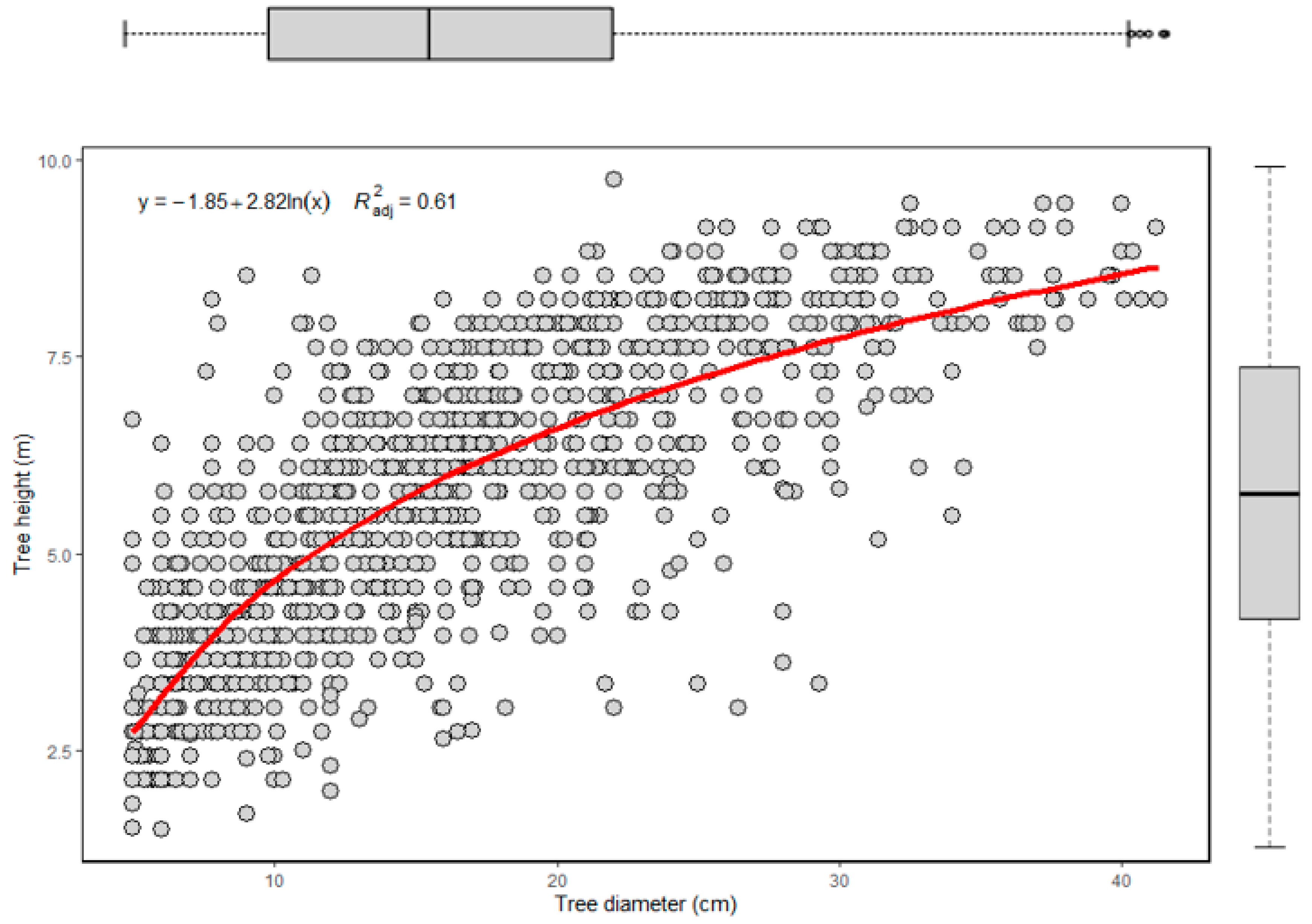
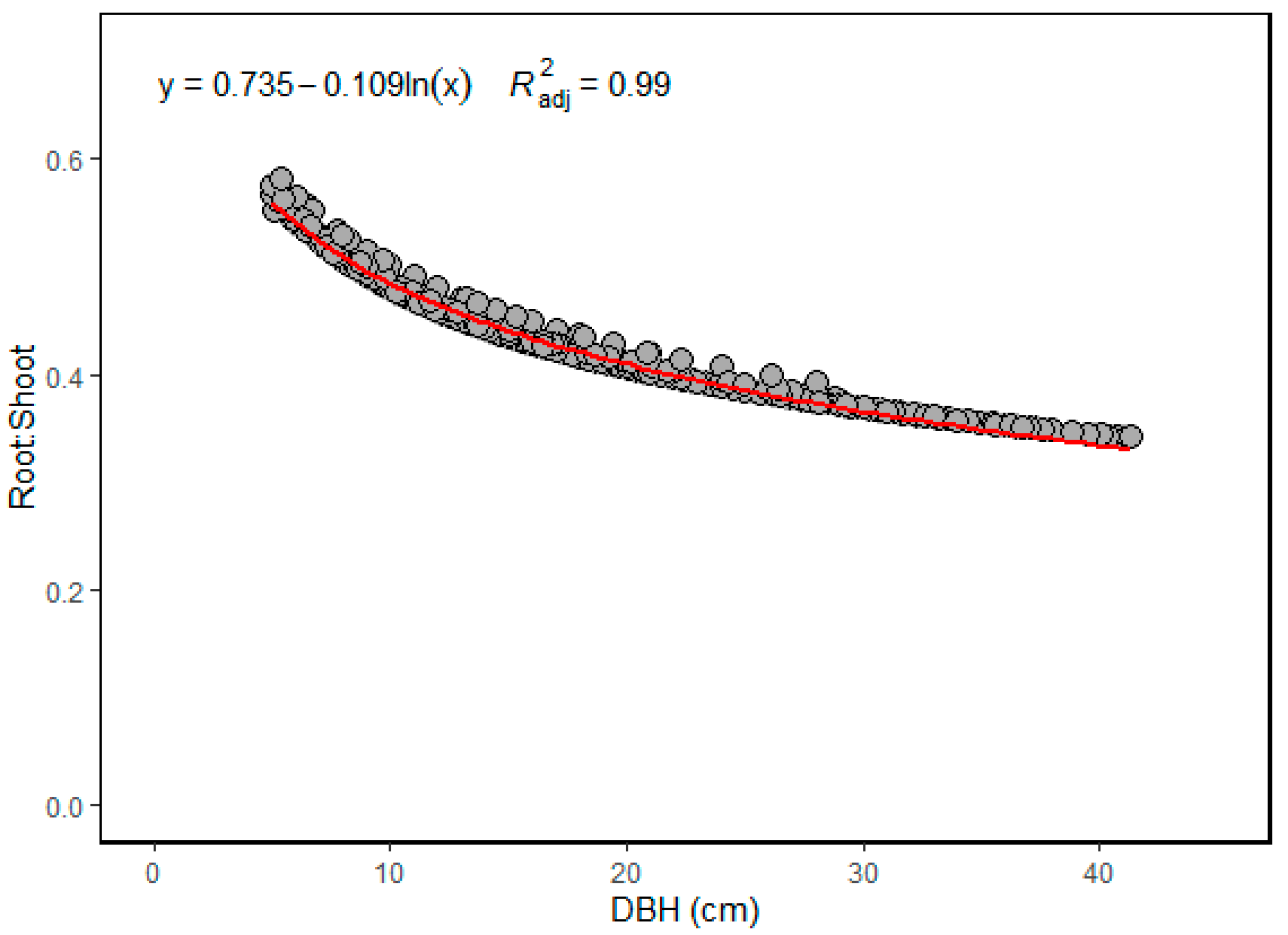
3.2. Structural Analysis

Important value index (IVI) was used to express the dominance and ecological success of any species with a single value; it was determined based on the total contribution of a species to the community by employing its relative density, relative basal area, and relative frequency in a study plot or area [42]. The more the number of individuals found, the higher density values. In the study site, the mangrove species of A. officinalis was found to have the highest average stem density (868 ± 463 ha−1) and highest relative density of 78.77%, followed by S. apetala (13.97%), S. caseolaris (4.17%) and Aegiceras corniculutum (2.90%). The least mean stem density was recorded by A. alba and Bruguirea sexangula (25 ± 0.00 ha−1). Frequency value of mangrove species is related to the number of plots where mangrove species are found. Here, A. officinalis has generally the highest frequency of presence in the study because this species has evenly distributed in each plot (Table 1). The relative frequency of Aegiceras corniculutum (11.36%) was higher than that of S. caseolaris (9.09%) because Aegiceras corniculutum was more evenly distributed than S. caseolaris (Table 1). High importance values were owned by the dominant species in a community. Here, A. officinalis showed the highest mean basal area (26.155 ± 16.940 m2 ha−1), contributing up to 87.66% of the total basal area, and had the highest important value index (IVI) of 218.69%, then followed by 45.53% for S. apetala, 15.97% for S. caseolaris, 15.06% for Aegiceras corniculutum, and 2.37% for A. alba and Bruguirea sexangula (Table 2). The highest value of importance index of A. officinalis explained that A. officinalis plays a relatively significant role in maintaining the sustainability of the mangrove ecosystem in the study area.
The genus Avicennia is a pioneer group of dominant plant species and mangrove plants in the genus Avicennia have both economic and ecological values [43]. A. officinalis (crypto viviparous) is widely distributed in Bangladesh, Cambodia, India, Indonesia, Malaysia, Myanmar, New Guinea, the Philippines, Sri Lanka, Thailand, Vietnam, and north-eastern Australia [40]. Avicennia species develop pencil-like pneumatophores, while Sonneratia species have thick cone-shaped pneumatophores. S. apetala species is also the pioneer species and mainly associated with A. officinalis species, [40,44,45]; they are growing on newly formed mudflats near the river mouth and found close to the sea. Therefore, mangrove species of A. officinalis and S. apetala play a vital role in reducing wave and tidal energy and retaining sediments. In Bangladesh, Aviecennia officinalis is planted with Sonneratia apetala for the coastal afforestation programme to protect the coastal community against tropical cyclones, storm surges, waves, tides, and saltwater intrusion. In the present study, A. officinalis and S. apetala have higher density, frequency, stand basal area, and importance values than other species of the mangrove stand; this condition showed that A. officinalis and S. apetala have high adaptive abilities in the mangrove stand of LetKhutKon Village.
Table 2. Tree species found in the mangrove stand of LetKhutKon Village (mean ± sd).
SpeciesMean Stem Density
(No. of Trees ha−1)
Mean BA
(m2 ha−1)
RD
(%)
RF
(%)
RBA (%)IVI
(%)
Avicennia officinalis868 ± 46326.155 ± 16.94078.7752.2787.66218.70
Sonneratia apetala154 ± 1622.633 ± 4.50313.9722.738.8345.53
Sonneratia caseolaris46 ± 1160.807 ± 1.9944.179.092.7115.97
Aegiceras corniculutum32 ± 840.238 ± 0.6462.9011.360.8015.06
Avicennia alba25 ± 0.00.0525 ± 0.0000.092.270.012.37
Bruguiera sexangula25 ± 0.00.050 ± 0.0000.092.270.012.37
RD is relative density; RF is relative frequency; RBA is relative basal area. The important value is calculated as IVI = RD + RF + RBA and IVI value can add up to a maximum value of 300 [46,47].
Shannon–Wiener index was used to estimate the diversity of species in the study area. The Shannon–Wiener’s diversity index (H′) was categorized as low with a value of 0.71 and the Shannon evenness index (SEI) was 0.40. Supporting the results of other studies were the Shannon–Wiener’s diversity index value of natural mangrove forest in the Mahanadi Mangrove Wetland (MMW), East Coast of India was 0.79 ± 0.38 [48], the mangrove of Lauhan village in East Java, Indonesia was 1.51 [24], and mangrove forest in Palawan, the Philippine was 0.99 [3]. Therefore, Shannon–Wiener’s diversity index (H′) value of the mangrove community of LetKhutKon Village was very low compared to other natural mangrove forests since the mangrove stand in the study site possessed a low number of mangrove species and was dominated by the few species. In contrast to tropical lowland rainforest, the mangroves have very low diversity as few plants have their special adaptations, which are attributed to their unique stands formation and harsh coastal habitat [8].

3.3. Biomass and Carbon Stock of Mangrove

Allometric method is the most widely used method for biomass estimation of the forest because this method provides non-destructive and less time-consuming than other methods [49]. In this study, the parameters of diameter at breast height (DBH) and wood density (ρ) were applied to compute mangrove biomass by using the allometric equations of Komiyama et al. [30]. As shown in Table 1, the overall mean biomass of the mangrove stand in LetKhutKon Village was found to be 335.55 ± 181.41 Mg ha−1 (the average aboveground biomass = 241.37 ± 132.73 Mg ha−1 and the average belowground biomass = 94.17 ± 48.73 Mg ha−1) wherein the total biomass produced was 8388.62 Mg ha−1. The reported AGB of mangroves in LetKhutKon Village (241.37 ± 132.73 Mg ha−1) was comparable to other mangroves, with the values of 255.7 Mg ha−1 reported in Lamu, Kenya [50], 246.90 Mg ha−1 at Guarás Island located in the state of Para [51] and 80.23 ± 15.95 t ha−1 at the Kerala state, the southwest corner of India [52]. There were considerable variations in the biomass between different species as shown in Table 3 and Table 4. Among the different species, the highest biomass of 7604.607 Mg ha−1 was recorded in A. officinalis (above and below-ground biomass were 5484.659 Mg ha−1 and 2119.947 Mg ha−1) and the lowest biomass was in Avicennia alba, having 0.333 Mg ha−1. The biomasses of remaining species such as S. apetala, S. caseolaris, Aegiceras cornoculutum, and Bruguiera sexangula were 597.564 Mg ha−1, 135.820 Mg ha−1, 49.898 Mg ha−1, and 0.397 Mg ha−1, respectively.
The aboveground biomass (AGB) and belowground biomass (BGB) contributed 71.93% and 28.07%, respectively, to the total mangrove biomass. The ratio of BGB to AGB (R:S ratio) ranged from 0.34 to 0.58 and the average ratio of BGB to AGB was 0.44 or 1:2.29. For comparison, the belowground biomass to aboveground biomass (R:S) ratio of mangroves was 0.46 or 1:2.17 in Kerala State, India [52] and 0.38 or 1:2.60 in Samar, the Philippines [3]. Mangrove forests have a higher root: shoot ratio (R: S) (generally R:S ratios between 0.33 or 1:3 and 0.50 or 1:2 [53]) when compared to the upland forests (R:S ratios between 0.22 or 1:4.52 and 0.25 or 1:3.96 [54]). Mangrove species are capable of allocating a high proportion of their total biomass to the belowground components which could be adapted to living in the soft sediments [53]. Figure 5 described the root: shoot (R:S) ratio against tree diameter at breast height (DBH in cm). Trees with DBH 10–21.98 cm had a mean R:S ratio of 0.44 while trees < 10 cm DBH had a mean R:S ratio of 0.52 and trees > 21.98 cm DBH had a value of 0.38. Our findings showed R:S ratio decreased significantly with increasing tree DBH.
The biomass of the plant is associated with the carbon-storing capacity of the plant [55], so estimating the biomass potential of mangrove vegetation can be used to calculate the carbon stock. The total carbon stock (C-stock) of the mangrove stand in LetKhutKon Village was 3754.304 Mg C ha−1 and varied from 17.37 Mg C ha−1 to as high as 373.06 Mg C ha−1 with a mean value of 150.25 ± 81.35 Mg C ha−1. The average C-stock of the mangrove stand was equivalent to carbon dioxide sequestration of 551.10 ± 298.64 Mg CO2 eq (1 ton of carbon = 3.67 tons of carbon dioxide) stored in the biomass. Total aboveground C-stock was 2836.12 Mg ha−1 and varied from 12.54 Mg C ha−1 to as high as 283.85 Mg C ha−1 with a mean value of 113.44 ± 62.38 Mg C ha−1. The belowground biomass was 2354.33 Mg ha−1 with an overall average of 94.17 ± 48.73 Mg ha−1 and the mean belowground C-stock was 36.73 ± 19.00 Mg C ha−1 (Table 1). The estimated biomass (335.54 ± 181.41 Mg ha−1) and stored carbon (150.17 ± 81.37 Mg C ha−1) of mangrove stand in the present study was higher than that of Labuan, Indonesia (168.05 Mg ha−1 and 74.7 Mg ha−1) [24], Kerala mangrove in Southwest Coast of India (117.1 t ha−1 and 139.82 t ha−1) [52], mangrove stand in the east coast of India (178.3 t ha−1 and 89.1 t ha−1) [48], and natural mangrove stands in Bohol Province, Philippines (323.6 t ha−1 and 145.6 t ha−1) [56]; however, the C-stock estimated in this study was lower than the C-stock obtained in the natural mangrove forest of Bahile, Puerto Princesa City, Palawan (757.7 t ha−1 and 356.1 t C ha−1) [57], and Thailand (345 t ha−1 and 155 t ha−1) [58]. The contribution of mangrove species to mean C-stock was in the following order: A. officinalis > S. apetala > S. caseolaris > Aegiceras corniculutum > Bruguiera sexangula > A. alba as shown in Table 3 and Table 4. Among the established sample plots, the highest biomass and C-stock were attributed in plot-9 with its corresponding maximum stand basal area of 69.125 m2 ha−1, whereas the lowest biomass and C-stock occurred in plot-24 with its corresponding minimum stand basal area of 26.692 m2 ha−1. Because plot 9 has the highest total DBH among the recorded sample plots; however, the DBH of trees measured in plot 24 was very low, since the trees were newly growing.

3.4. The Relationships between Carbon Density and Structural Variables

Pearson’s correlation coefficient was used to see the relationship between the variables at a 95% confidence interval. The correlations between the predictor variables and the dependent variable were shown in Table 5. Aboveground carbon stock (AGC) was positively correlated with all structural variables such as mean DBH ( D ¯ ), mean height   ( H ¯ ) , and stand basal area (BA). AGC was positively associated with BA (R = 0.9921, p < 2.2 × 10⁻¹⁶), mean DBH (R = 0.8033, p = 3.94 × 10−06) and mean height (R = 0.6838, p = 3.21 × 10−04); this finding indicated that basal area was a significant predictor of the aboveground carbon-stock of trees in the mangrove stand.

3.5. Influence of Structural Variables on Aboveground Carbon-Stock

Linear regression analysis was performed to describe the relationship between stand-level carbon stocks (Mg C ha−1) as the dependent variable and stand structural parameters such as mean DBH, mean H and basal area as independent variables. All models were named and described in Table 6. As specified in the Table, carbon stock was significantly correlated with structural variables. Through the linear regression analysis, we found that carbon stored in the tree biomass was influenced by forest structural characteristics.
Model (1) analyzed the relationship between aboveground carbon stock-AGC (Mg C ha−1) and mean diameter at breast height. The model had R2-adj = 0.6792, AIC = 10.570, BIC = 13.977, RMSE = 0.267 and p = 8.14 × 10−07. As mean DBH increased by 1 cm, on an average aboveground carbon stock increased by 2.1231 Mg ha−1 keeping all things constant; it showed AGC had a direct correlation with DBH, therefore it could be assumed that DBH was a reliable dendrometric variable for aboveground carbon stock estimation [59,60,61]. The mangrove tree biomass model, which was determined from DBH, only had a practical advantage because most of the inventories included DBH measurements. Furthermore, it was easy to measure accurately in the field.
ln ( AGC ) = 1.3088 + 2.1231   ln ( D ¯ )
The relationship between aboveground carbon stock-AGC (Mg ha−1) and mean height (m) was assessed in model 2; this model had a coefficient of determination of 0.4625 and the parameters were statistically significant (p = 0.0002142). Although AGC had a significant positive relationship with Mean H, it showed a lower R2-adj (46.25%), higher AIC (22.440), and higher BIC (25.847) when compared with the relationship between AGC and mean DBH; thus, mean height (m) as an individual independent variable was deniable as one of the important predictors for the estimation of AGC.
ln ( AGC ) = 1.3728 + 1.8867   ln ( H ¯ )
The result of the linear regression analysis of the model (3) revealed that aboveground carbon stock density (Mg ha−1) had a significant, positive relationship with stand basal area (m2 ha−1) with a coefficient of determination of 0.9834; parameters were statistically significant (p < 2.2 × 10⁻¹⁶). The result was statistically interpreted, as the stand basal area increased by 1 m2 ha−1, and on an average above-ground carbon stock increased by 1.21227 Mg ha−1 keeping all things constant. The strong relationship between stand basal area and aboveground carbon stock is because both variables have been associated with the diameter of a tree trunk; it means if the size of the tree trunk increases, the stand basal area increases because tree basal area is the cross-sectional area of a tree trunk measured at the breast height over bark, and as a consequence, the aboveground biomass and carbon stock also increase.
ln(AGC)= 0.58368 + 1.21227 ln(BA)
Across all structural variables, stand-level carbon stock showed the highest relationship (R2 adj = 97.21, p < 2.2 × 10⁻¹⁶) with the stand basal area. When the stand basal area and tree height were used as compound variables in the model, it explained 97.28% of carbon variation. Model (4) has appeared the best fit model showing fitting statistics (R2 = 97.28, AIC = −5.350, BIC = −40.808, RMSE = 0.076, p-value < 2.2 × 10⁻¹⁶) and very close to model 3. Despite that fact, both models (3 and 4) were still able to explain carbon storage very well (Adj. R2 > 90%).
In   ( AGC ) = 0.46971 + 1.16254   ln ( BA ) + 0.16235   ln ( H ¯ )
For a better analysis of residual distribution, we used the respective statistical test for checking the models. We ran the Durbin–Watson test to detect the autocorrelation in the residuals. The test statistics were for model 3: DW = 1.7032, p-value = 0.2052 and for model 4: DW = 1.5571, p-value = 0.1014. For both models, the presence of autocorrelation was not significant as the p-value > 0.05 and the value of DW ~ 2. We further ran the Shapiro–Wilk test for normality and both models were normality distributed (p-value = 0.8458 and 0.7164 for model 3 and model 4 respectively). Additionally, we performed Breusch–Pagan test (bptest) to determine whether heteroscedasticity was present in the regression model. The test statistics concluded there may not be heteroscedasticity as the p-value > 0.05; thus, the best fit equations for estimating stand-level carbon stock were Model 3: ln(AGC) = 0.58368 + 1.21227 ln(BA), one-variable model using stand basal area (m2 ha−1) as predicted variable, and Model 4: In(AGC) = 0.46971 + 1.16254 ln(BA) + 0.16235 ln ( H ¯ ) , two-variable model using stand basal area and mean height (m2, m).

4. Conclusions

By applying the non-destructive methodology, biomass and carbon stock of the mangrove stand of Kanhlyashay natural mangrove forest were estimated. A low diversity index value (H′ = 0.71) was observed in the natural mangrove stand that was dominated by the species of Aviecennia officinalis (IVI = 218.69%) from Acanthaceae family comprised 78.77% of the total tree count. Therefore, A. officinalis has high adaptive abilities in the mangrove stand of LetKhutKon Village. Pioneer mangrove species such as Avicennia officinalis and Sonneratia caseolaris have a good survival rate on the mudflats, and they are suitable mangrove species for mangrove afforestation on unoccupied mudflats because of their tolerance to increased salinity. The total biomass and carbon stock in the natural mangrove forest were 335.55 ± 181.41 Mg ha−1 and 150.25 ± 81.37 Mg C ha−1, where the above and below-ground carbon stock contributed 71.93% and 28.07%, respectively. Stand-level allometric equations in the estimation of aboveground carbon stock were implicated. The finding revealed that the one-variable model of the stand basal area and the two-variables model (basal area + mean height) were suitable based on fitting statistics and certain statistical tests for high-precision estimates of stand-level carbon stock of Mangrove stand in the study site. Our observation highlights the natural mangrove forest in the study site has the potential to store and sequester a significant amount of carbon. Because natural mangrove forest in the study site is a young age stand and is dominated by the fast-growing pioneer species. At a young age stand, the rate of carbon sequestration is high. In addition to the stand age, the rate of carbon uptake of the forest ecosystem depends on forest management. Therefore, forest management activities are necessary to maintain forest carbon sequestration capacity.

Author Contributions

Conceptualization, W.N.A. and X.T.; data collection, methodology, validation, formal analysis, data curation, writing—original draft preparation, W.N.A.; writing—review and editing, W.N.A., X.T. and A.W.T.; supervision, X.T. All authors contributed critically to the drafts and gave final approval for publication. All authors have read and agreed to the published version of the manuscript.

Funding

Article Processing Charge(APC) was funded by National Natural Science Foundation of China (31872703).

Acknowledgments

The authors gratefully acknowledge APFNet Scholarship funding the first author’s research at Beijing Forestry University. The authors thank to everyone who helped with the field survey and the anonymous reviewers for their valuable comments.

Conflicts of Interest

The authors declare no conflict of interest.

References

  1. Myint, S.W.; Giri, C.P.; Wang, L.; Zhu, Z.; Gillette, S.C. Identifying Mangrove Species and Their Surrounding Land Use and Land Cover Classes Using an Object-Oriented Approach with a Lacunarity Spatial Measure. GISci. Remote Sens. 2008, 45, 188–208. [Google Scholar] [CrossRef]
  2. Naylor, L.A.; Viles, H.; Carter, N.E.A. Biogeomorphology revisited: Looking towards the future. Geomorphology 2002, 47, 3–14. [Google Scholar] [CrossRef]
  3. Abino, A.C.; Castillo, J.A.A.; Lee, Y.J. Assessment of species diversity, biomass and carbon sequestration potential of a natural mangrove stand in Samar, the Philippines. For. Sci. Technol. 2014, 10, 2–8. [Google Scholar] [CrossRef]
  4. Alongi, D.M. Present state and future of the world’s mangrove forests. Environ. Conserv. 2002, 29, 331–349. [Google Scholar] [CrossRef] [Green Version]
  5. Donato, D.C.; Kauffman, J.B.; Murdiyarso, D.; Kurnianto, S.; Stidham, M.; Kanninen, M. Mangroves among the most carbon-rich forests in the tropics. Nat. Geosci. 2011, 4, 293–297. [Google Scholar] [CrossRef]
  6. Lovelock, C.E. Soil Respiration and Belowground Carbon Allocation in Mangrove Forests. Ecosystems 2008, 11, 342–354. [Google Scholar] [CrossRef]
  7. Alongi, D.M. Mangrove forests: Resilience, protection from tsunamis, and responses to global climate change. Estuar. Coast. Shelf Sci. 2008, 76, 1–13. [Google Scholar] [CrossRef]
  8. Rasquinha, D.N.; Mishra, D.R. Tropical cyclones shape mangrove productivity gradients in the Indian subcontinent. Sci. Rep. 2021, 11, 1–12. [Google Scholar] [CrossRef]
  9. Alongi, D.M. Carbon Cycling and Storage in Mangrove Forests. Annu. Rev. Mar. Sci. 2014, 6, 195–219. [Google Scholar] [CrossRef]
  10. Bhomia, R.K.; Kauffman, J.B.; McFadden, T.N. Ecosystem carbon stocks of mangrove forests along the Pacific and Caribbean coasts of Honduras. Wetl. Ecol. Manag. 2016, 24, 187–201. [Google Scholar] [CrossRef]
  11. Alongi, D.M. Global Significance of Mangrove Blue Carbon in Climate Change Mitigation. Science 2020, 2, 67. [Google Scholar] [CrossRef]
  12. Kankare, V.; Vastaranta, M.; Holopainen, M.; Räty, M.; Yu, X.; Hyyppä, J.; Hyyppä, H.; Alho, P.; Viitala, R. Retrieval of Forest Aboveground Biomass and Stem Volume with Airborne Scanning LiDAR. Remote Sens. 2013, 5, 2257–2274. [Google Scholar] [CrossRef] [Green Version]
  13. Kosoy, N.; Corbera, E. Payments for ecosystem services as commodity fetishism. Ecol. Econ. 2010, 69, 1228–1236. [Google Scholar] [CrossRef]
  14. Friess, D.A.; Rogers, K.; Lovelock, C.E.; Krauss, K.W.; Hamilton, S.E.; Lee, S.Y.; Lucas, R.; Primavera, J.; Rajkaran, A.; Shi, S. The State of the World’s Mangrove Forests: Past, Present, and Future. Annu. Rev. Environ. Resour. 2019, 44, 89–115. [Google Scholar] [CrossRef] [Green Version]
  15. Veettil, B.K.; Pereira, S.F.R.; Quang, N.X. Rapidly diminishing mangrove forests in Myanmar (Burma): A review. Hydrobiologia 2018, 822, 19–35. [Google Scholar] [CrossRef]
  16. Spalding, M. World Atlas of Mangroves; Routledge: London, UK, 2010; ISBN 9781849776608. [Google Scholar]
  17. Oo, N. Present state and problems of mangrove management in Myanmar. Trees 2002, 16, 218–223. [Google Scholar] [CrossRef]
  18. De Alban, J.D.T.; Jamaludin, J.; de Wen, D.W.; Than, M.M.; Webb, E.L. Improved estimates of mangrove cover and change reveal catastrophic deforestation in Myanmar. Environ. Res. Lett. 2020, 15, 034034. [Google Scholar] [CrossRef]
  19. GGGI MM03 Mangrove Restoration Program in Myanmar—Global Green Growth Institute. Available online: https://gggi.org/project/project-reference-profiles-myanmarmm03-mangrove-restoration-program-in-myanmar/ (accessed on 29 November 2021).
  20. Aye, W.N.; Wen, Y.; Marin, K.; Thapa, S.; Tun, A.W. Contribution of Mangrove Forest to the Livelihood of Local Communities in Ayeyarwaddy Region, Myanmar. Forests 2019, 10, 414. [Google Scholar] [CrossRef] [Green Version]
  21. Galidaki, G.; Zianis, D.; Gitas, I.; Radoglou, K.; Karathanassi, V.; Tsakiri–Strati, M.; Woodhouse, I.; Mallinis, G. Vegetation biomass estimation with remote sensing: Focus on forest and other wooded land over the Mediterranean ecosystem. Int. J. Remote Sens. 2017, 38, 1940–1966. [Google Scholar] [CrossRef] [Green Version]
  22. Hashim, T.; Suratman, M.N. Mangrove Biomass: Review on Estimation Methods and the Applications of Remote Sensing Approach; Mangroves; FRIM: Kuala Lumpr, Malaysia, 2020. [Google Scholar]
  23. DMH. Department of Meteorology and Hydrology. Available online: https://www.moezala.gov.mm/ (accessed on 15 November 2021).
  24. Asadi, M.A.; Yona, D.; Saputro, S.E. Species Diversity, Biomass, and Carbon Stock Assessments of Mangrove Forest in Labuhan, Indonesia. In Proceedings of the IOP Conference Series: Earth and Environmental Science; IOP Publishing: Bristol, UK, 2018; Volume 151. [Google Scholar]
  25. Shannon, C.E.; Weaver, W. The Mathematical Theory of Communication; University of Illinois Press: Urbana, IL, USA, 1963; ISBN 9780252725487. [Google Scholar]
  26. Gevaña, D.; Pampolina, N.M. Plant Diversity and Carbon Storage of a Rhizopora Stand in Verde Passage, San Juan, Batangas, Philippines. J. Environ. Sci. Manag. 2010, 12, 1–10. [Google Scholar]
  27. Sharma, C.M.; Baduni, N.P.; Gairola, S.; Ghildiyal, S.K.; Suyal, S. Tree diversity and carbon stocks of some major forest types of Garhwal Himalaya, India. For. Ecol. Manag. 2010, 260, 2170–2179. [Google Scholar] [CrossRef]
  28. Lumbres, R.I.C.; Palaganas, J.A.; Micosa, S.C.; Laruan, K.A.; Besic, E.D.; Yun, C.-W.; Lee, Y.-J. Floral diversity assessment in Alno communal mixed forest in Benguet, Philippines. Landsc. Ecol. Eng. 2014, 10, 361–368. [Google Scholar] [CrossRef]
  29. Wim, G.; Stephan, W.; Max, Z.; Liesbeth, S. Mangrove Guidebook Forsoutheastasia; FAO Regional Office for Asia and the Pacific: Bangkok, Thailand, 2006; ISBN 9747946858. [Google Scholar]
  30. Komiyama, A.; Poungparn, S.; Kato, S. Common allometric equations for estimating the tree weight of mangroves. J. Trop. Ecol. 2005, 21, 471–477. [Google Scholar] [CrossRef]
  31. Chave, J.; Coomes, D.; Jansen, S.; Lewis, S.L.; Swenson, N.G.; Zanne, A.E. Towards a worldwide wood economics spectrum. Ecol. Lett. 2009, 12, 351–366. [Google Scholar] [CrossRef]
  32. FAO. State of the World’s Forests 2011; Food and Agriculture Organization of the United Nations: Rome, Italy, 2011. [Google Scholar]
  33. IPCC 2006 IPCC Guidelines for National Greenhouse Gas Inventories—IPCC. Available online: https://www.ipcc.ch/report/2006-ipcc-guidelines-for-national-greenhouse-gas-inventories/ (accessed on 17 September 2021).
  34. Feldpausch, T.R.; Rondon, M.A.; Fernandes, E.C.M.; Riha, S.J.; Wandelli, E. Carbon and Nutrient Accumulation in Secondary Forests Regenerating on Pastures in Central Amazonia. Ecol. Appl. 2004, 14, 164–176. [Google Scholar] [CrossRef] [Green Version]
  35. Kauffman, J.B.; Donato, D.C. Protocols for the Measurement, Monitoring and Reporting of Structure, Biomass and Carbon Stocks in Mangrove Forests; CFIOR: Bogor, Indonesia, 2012. [Google Scholar] [CrossRef]
  36. Kauffman, J.B.; Arifanti, V.B.; Basuki, I.; Kurnianto, S.; Novita, N.; Murdiyarso, D.; Donato, D.C.; Warren, M.W. Protocols for the Measurement, Monitoring, and Reporting of Structure, Biomass, Carbon Stocks and Greenhouse Gas Emissions in Tropical Peat Swamp Forests; Center for International Forestry Research: Bogor, Indonesia, 2016. [Google Scholar] [CrossRef]
  37. Baskerville, G.L. Use of Logarithmic Regression in the Estimation of Plant Biomass. Can. J. For. Res. 1972, 2, 49–53. [Google Scholar] [CrossRef]
  38. Altanzagas, B.; Luo, Y.; Altansukh, B.; Dorjsuren, C.; Fang, J.; Hu, H. Allometric Equations for Estimating the Above-Ground Biomass of Five Forest Tree Species in Khangai, Mongolia. Forests 2019, 10, 661. [Google Scholar] [CrossRef] [Green Version]
  39. Sprugel, D.G. Correcting for Bias in Log-Transformed Allometric Equations. Ecology 1983, 64, 209–210. [Google Scholar] [CrossRef]
  40. Edwards, P.J.; Tomlinson, P.B. The Botany of Mangroves. Kew Bull. 1986, 42. [Google Scholar] [CrossRef]
  41. Zöckler, C.; Aung, C. The Mangroves of Myanmar. In Sabkha Ecosystems; Springer: Berlin/Heidelberg, Germany, 2019; pp. 253–268. [Google Scholar] [CrossRef]
  42. Faridah-Hanum, I.; Kudus, K.A.; Saari, N.S. Plant Diversity and Biomass of Marudu Bay Mangroves in Malaysia. Pakistan J. Bot. 2012, 44, 151–156. [Google Scholar]
  43. Thatoi, H.; Samantaray, D.; Das, S.K. The genus Avicennia, a pioneer group of dominant mangrove plant species with potential medicinal values: A review. Front. Life Sci. 2016, 9, 267–291. [Google Scholar] [CrossRef] [Green Version]
  44. Duke, N. Phenologies and Litter Fall of Two Mangrove Trees, Sonneratia alba Sm. and S. caseolaris (L.) Engl., And Their Putative Hybrid, S. × Gulngai N.C. Duke. Aust. J. Bot. 1988, 36, 473–482. [Google Scholar] [CrossRef]
  45. Nasrin, S.; Hossain, M.; Alam, R.M. A Monograph on Sonneratia Apetala Buch.-Ham.; Lap Lambert Academic Publishing: Saarbrücken, Germany, 2017; ISBN 3330052511. [Google Scholar]
  46. Schaefer-Novelli, C.; Cintron, G.; Novelli, Y.S. Methods for Studying Mangrove Structure. In The Mangrove Ecosystem: Research Methods; Snedaker, S.C., Snedaker, J.G., Eds.; United Nations Educational, Scientific and Cultural Organization: Paris, France, 1984; pp. 91–113. Available online: http://www.sciepub.com/reference/14979 (accessed on 2 December 2021).
  47. Curtis, J.T.; McIntosh, R.P. The Interrelations of Certain Analytic and Synthetic Phytosociological Characters. Ecology 1950, 31, 434–455. [Google Scholar] [CrossRef]
  48. Sahu, S.C.; Kumar, M.; Ravindranath, N.H. Carbon Stocks in Natural and Planted Mangrove forests of Mahanadi Mangrove Wetland, East Coast of India. Curr. Sci. 2016, 110, 2253–2260. [Google Scholar] [CrossRef]
  49. Kridiborworn, P.; Chidthaisong, A.; Yuttitham, M.; Tripetchkul, S. Carbon Sequestration by Mangrove Forest Planted Specifically for Charcoal Production in Yeesarn, Samut Songkram. J. Sustain. Energy Environ. 2012, 3, 87–92. [Google Scholar]
  50. Kairo, J.; Mbatha, A.; Murithi, M.M.; Mungai, F. Total Ecosystem Carbon Stocks of Mangroves in Lamu, Kenya; and Their Potential Contributions to the Climate Change Agenda in the Country. Front. For. Glob. Chang. 2021, 4, 151. [Google Scholar] [CrossRef]
  51. Salum, R.B.; Souza-Filho, P.W.M.; Simard, M.; Silva, C.A.; Fernandes, M.E.B.; Cougo, M.F.; Do Nascimento, W.; Rogers, K. Improving mangrove above-ground biomass estimates using LiDAR. Estuar. Coast. Shelf Sci. 2020, 236, 106585. [Google Scholar] [CrossRef]
  52. Harishma, K.M.; Sandeep, S.; Sreekumar, V.B. Biomass and carbon stocks in mangrove ecosystems of Kerala, southwest coast of India. Ecol. Process. 2020, 9, 1–9. [Google Scholar] [CrossRef]
  53. Komiyama, A.; Ong, J.E.; Poungparn, S. Allometry, biomass, and productivity of mangrove forests: A review. Aquat. Bot. 2008, 89, 128–137. [Google Scholar] [CrossRef]
  54. Cairns, M.A.; Brown, S.; Helmer, E.H.; Baumgardner, G.A. Root biomass allocation in the world’s upland forests. Oecologia 1997, 111, 1–11. [Google Scholar] [CrossRef]
  55. O’Connor, E. ENERGY CROPS | Biomass Production. In Encyclopedia of Applied Plant Sciences; Elsevier: Amsterdam, The Netherlands, 2003; pp. 266–273. [Google Scholar]
  56. Camacho, L.D.; Gevaña, D.T.; Carandang, A.P.; Camacho, S.C.; Combalicer, E.A.; Rebugio, L.L.; Youn, Y.-C. Tree biomass and carbon stock of a community?managed mangrove forest in Bohol, Philippines. For. Sci. Technol. 2011, 7, 161–167. [Google Scholar] [CrossRef]
  57. Abino, A.C.; Lee, Y.J.; Castillo, J.A.A. Species Diversity, Biomass, and Carbon Stock Assessments of a Natural Mangrove Forest in Palawan, Philippines. Pakistan J. Bot. 2014, 46, 1955–1962. [Google Scholar]
  58. Jachowski, N.R.A.; Quak, M.S.Y.; Friess, D.A.; Duangnamon, D.; Webb, E.L.; Ziegler, A.D. Mangrove biomass estimation in Southwest Thailand using machine learning. Appl. Geogr. 2013, 45, 311–321. [Google Scholar] [CrossRef]
  59. Brahma, B.; Nath, A.J.; Deb, C.; Sileshi, G.W.; Sahoo, U.K.; Das, A.K. A critical review of forest biomass estimation equations in India. Trees For. People 2021, 5, 100098. [Google Scholar] [CrossRef]
  60. Ghasemi, A.; Fallah, A.; Joibary, S.S. Allometric equations for estimating standing biomass of Avicennia marina in Bushehr of Iran. Off. J. İstanbul Univ.-Cerrahpaşa Fac. For. 2016, 66, 691–697. [Google Scholar] [CrossRef]
  61. Kebede, B.; Soromessa, T. Allometric equations for aboveground biomass estimation of Olea europaea L. subsp. cuspidatain Mana Angetu Forest. Ecosyst. Health Sustain. 2018, 4, 1–12. [Google Scholar] [CrossRef] [Green Version]
Figure 1. Location of the study site and sampling points in the mangrove stand of Kanhlyashay natural mangrove forest.
Forests 13 01013 g001
Figure 2. Species Distribution of Mangrove stands in LetKhutKon Village.
Forests 13 01013 g002
Figure 3. Tree abundance and number of species found in different plots in the mangrove stand of LetKhutKon Village.
Forests 13 01013 g003
Figure 4. Scatter plot of tree height vs diameter in the mangrove stand of LetKhutKon Village.
Forests 13 01013 g004
Figure 5. Root: Shoot (R:S) ratios against tree diameter at breast height (DBH in cm).
Forests 13 01013 g005
Table 1. Distribution of stand density, biomass, carbon stock, and CO2 equivalent in the natural mangrove stand, LetKhutKon Village.
PlotStand Density (Stems ha−1)SpeciesDBH Range
(cm)
Height Range
(m)
Basal Area
(m2 ha−1)
Biomass (Mg ha−1)C-Stock
Mg C ha−1
CO2 Equivalent
(MgCO2 eq)
AGBBGBTB
11250Ao, Sa5.00–29.003.05–9.7519.950131.07755.307186.3883.18305.26
21125Ao, Sa8.00–34.003.05–8.2321.725145.76961.048206.8292.32338.82
3875Ao, Sa5.50–34.002.44–7.9326.000214.80783.486298.29135.52490.01
4875Ao5.00–35.302.13–8.5319.375159.38162.136221.5299.14363.14
5875Ao5.20–31.802.74–8.2325.725211.05582.610293.67131.41482.29
6875Ao5.30–37.002.74–8.2333.900294.506111.881406.39182.05668.13
7625Ao16.40–40.005.18–9.4542.950405.162147.636552.80248.00910.18
81000Ao5.50–40.702.74–9.1447.750425.534159.583585.12262.24962.42
91625Ao7.60–41.203.05–9.1469.125603.928228.753832.68373.061369.13
101000Ao6.60–37.204.27–9.5030.025248.52596.739345.26154.54567.14
111125Ao6.00–40.103.66–9.4541.025352.219134.529486.75218.01800.09
12750Ao6.10–39.503.35–9.1429.575259.83598.089357.92160.38588.58
131375Ao5.00–41.303.05–9.1451.650446.873170.086616.96276.361014.26
141525Ac, Ao, Sa5.00–26.602.13–8.2317.075113.65849.255162.9172.63266.55
151075Ao, Sa5.90–28.802.13–9.1424.325187.26075.120262.38117.31430.52
161875Ao, Sa, Sc5.10–35.602.13–9.5041.225302.509121.188423.70189.44695.26
17975Ao5.50–38.802.13–8.8430.275258.54299.003357.55160.13587.66
182025Ao5.40–37.602.13–9.1443.800346.801138.028484.83216.83795.76
191075Ao6.10–29.003.66–8.8422.900171.74770.439242.19108.19397.07
20925Ao8.30–23.503.35–8.2317.750126.14853.263179.4180.06293.83
211175Ao, Sa, Sc6.50–37.002.13–7.6230.025229.08291.594320.68143.39526.24
221075Ac, Aa, Ao,
Bs, Sc
5.10–36.701.70–7.9322.875166.66566.580233.25104.30382.78
23950Ac, Ao, Sa5.00–31.001.50–6.8617.200122.80149.746172.5577.12283.02
24550Ac, Sa5.00–17.002.13–5.494.92526.69112.36339.0517.3763.73
25950Ac, Sa, Sc5.50–25.902.44–7.6214.80083.71335.868119.5853.33195.73
Mean6.22–33.942.76–8.5329.838241.37294.173335.55150.25551.10
Standard deviation2.32–6.260.84–0.9614.032132.73148.728181.4181.35298.64
Note: Ao-Avicennia officinalis; So-Sonneratia caseolaris; Sa-Sonneratia apetala; Ac-Aegiceras corniculatum; Bs-Bruguiera sexangula; Aa-Avicennia alba.
Table 3. Biomass and carbon stock differences among the species in the mangrove stand.
SpeciesBiomass (Mg ha−1)C-Stock (Mg C ha−1)
AGBBGBAGCBGC
Avicennia officinalis5484.6592119.9472577.790826.779
Sonneratia apetala420.535177.029197.65169.041
Sonneratia caseolaris94.67241.14844.49616.048
Aegiceras corniculutum33.95115.94715.9576.219
Avicennia alba0.2130.1200.1000.047
Bruguiera sexangula0.2560.1410.1200.055
Table 4. Mean diameter breast height, biomass, and carbon stock of recorded mangrove species in mangrove stands of LetKhutKon Village (mean ± sd).
SpeciesMean DBHBiomass (Mg ha−1)Vegetation Carbon Stock (Mg C ha−1)
AGBBGBTBAGCBGCTVC
Avicennia officinalis17.66 ± 8.476.319 ± 6.8882.442 ± 2.4258.761 ± 9.3122.970 ± 3.2370.953 ± 0.9463.922 ± 4.183
Sonneratia apetala13.43 ± 6.132.731 ± 2.8851.150 ± 1.1053.880 ± 3.9891.283 ± 1.3560.448 ± 0.4311.732 ± 1.787
Sonneratia caseolaris13.81 ± 5.792.058 ± 2.1810.895 ± 0.8532.953 ± 3.0340.967 ± 1.0250.349 ± 0.3331.316 ± 1.358
Aegiceras corniculutum9.24 ± 3.081.061 ± 0.8360.498 ± 0.3571.559 ± 1.1920.499 ± 0.3930.194 ± 0.1390.693 ± 0.532
Avicennia alba5.200.213 0.120 0.332 0.100 0.047 0.147
Bruguiera sexangula5.100.256 0.141 0.397 0.120 0.055 0.175
Total16.64 ± 8.235.476 ± 6.4382.136 ± 2.2797.612 ± 8.7162.574 ± 3.0260.833 ± 0.8893.407 ± 3.914
Table 5. Pearson’s correlation coefficients between aboveground carbon (AGC) density and structural parameters of the stand.
Structural VariablesPearson Correlation Coefficient with AGC
(Mg C ha−1)
p-Value
Mean DBH (cm)0.80333.94 × 10−06
Mean H (m)0.68383.21 × 10−04
BA (m2/ha)0.9921<2.2 × 10−16
Table 6. Linear regression analysis result of stand structural variables and aboveground carbon stock (AGC).
ModelAdj. R2 (%)RMSEAICBICbptestCFp-Value
Model 167.920.26710.57013.9770.5211.03988.14 × 10−07
Model 246.250.34622.44025.8470.3821.06770.000214
Model 397.210.079−45.586−42.1800.2301.0034<2.2 × 10⁻¹⁶
Model 497.280.076−45.350−40.8080.1871.0033<2.2 × 10⁻¹⁶
Note: Model 1: one-variable (mean DBH (cm)), Model 2: one-variable (mean Height, (m)), Model 3: one-variable (basal area, (m2)), Model 4: two-variable (BA, H ¯ (m2, m)). The statistics represent the coefficient of determination (R2-adj), Root Mean Square Error (RMSE), Akaike information criterion (AIC), Bayesian Information Criterion (BIC), bptest, Correction factor (CF) and p-value.
Publisher’s Note: MDPI stays neutral with regard to jurisdictional claims in published maps and institutional affiliations.

