Article

Friction Coefficients of Chestnut (Castanea sativa Mill.) Sawn Timber for Numerical Simulation of Timber Joints

by
José Ramón Villar-García
1,*,
Pablo Vidal-López
2,
Desirée Rodríguez-Robles
2 and
Manuel Moya Ignacio
1
1
Forest Research Group, Department of Forest and Agricultural Engineering, Universitary Center of Plasencia, University of Extremadura, Av. Virgen del Puerto 2, 10600 Plasencia, Spain
2
Mechanical and Fluid Engineering Research Group, Department of Forest and Agricultural Engineering, School of Agricultural Engineering, University of Extremadura, Av. Adolfo Suarez s/n, 06071 Badajoz, Spain
*
Author to whom correspondence should be addressed.
Forests 2022, 13(7), 1078; https://doi.org/10.3390/f13071078
Submission received: 30 May 2022 / Revised: 1 July 2022 / Accepted: 8 July 2022 / Published: 9 July 2022
(This article belongs to the Section Wood Science and Forest Products)

Abstract

:
This study focuses on the friction characteristics of chestnut sawn timber (Castanea sativa Mill.) of Spanish origin. The values of both the static and dynamic friction coefficients were determined, as this knowledge is of interest for the numerical simulation of the stress transmission in joints of timber structures. Therefore, two sets of tests were carried out combining different orthotropic orientations. Firstly, timber-to-timber tests were assessed to obtain the coefficients applicable to carpentry joints; secondly, timber-to-steel friction was also evaluated to determine the coefficients needed for mechanical joints with metal plates and dowels. The results presented a conventional behavior of friction, i.e., a maximum static value before sliding and a subsequent decrease. For timber-to-timber tests, global mean values of μs = 0.47 and μk = 0.36 were found, and the results were slightly higher than those obtained between pieces with the same orthotropic orientation and sliding direction. Regarding timber-to-steel tests, the resulting friction coefficients, as well as the difference existing between the static and dynamic values were lower (μs = 0.19 and μk = 0.17) compared to the timber-to-timber sets. The use of these results in numerical studies would allow for closer simulations in which chestnut wood is involved in friction. In addition, the values provided herein could be included as new data in standards that already consider other wood species.

1. Introduction

Wood is one of the oldest construction materials employed by humanity, and it is still widely used in the construction industry both due to its intrinsic mechanical properties and aesthetic value, and more recently due to its sustainability potential.
Since wood is a natural material, certain properties are greatly variable and can be complex to manage in engineering settings. Nonetheless, it is widely recognized that properties within a specific species are relatively constant. As such, different wood species are regarded as better than others for construction purposes.
There is a vast tradition in the use of chestnut wood (Castanea sativa, Mills.) for structural purposes in the southern countries of Europe, such as Spain. Proof of that is in the numerous constructions that have reached the present time and use this material mainly for beams and columns. Despite its recognized durability [1,2], this kind of building is currently undergoing maintenance and rehabilitation, thus requiring this same type of wood for functional and aesthetic reasons. Moreover, in recent years, there has been a surge in the demand of hardwood for structural applications. Figure 1 shows the evolution of the production, trade and consumption of sawn hardwood in Europe, thus illustrating the aforementioned tendency, although it should be noted that the 2020 decrease reflects the context of the COVID-19 pandemic. In addition, the development of computer-aided manufacture could also be credited as a driver in the increase of sawn hardwood consumption since it favors more economical carpentry joints. In this regard, Carbone et al. [3] conducted a study regarding the competitiveness of chestnut timber laminated products. The authors reported a promising future for this type of wood but indicated the need for a dedicated chestnut wood policy to further promote the markets. For instance, in Spain, UNE 56546 [4] regulates the visual grading for structural sawn hardwood timber of Spanish origin, and it is regarded as a point forward to a greater presence of laminated chestnut wood products on the market.
Chestnut is part of the Fagaceae family, which also includes beech and oak. It is the only native species of the Castanea genus in Europe, and it is mostly distributed in the Mediterranean basin (Figure 2), covering more than 2.5 million hectares [6]. For instance, in Spain, it is estimated to cover 163,164.5 ha [7] and to be mostly located in the north provinces (Galicia, Asturias, Navarre and Catalonia), but it also can be found dispersed in the center and south of the country.
As a multipurpose species, chestnut is valued both for fruit and non-wood products as well as timber, although the latter entails up to 79% of its growing area [6]. Besides its easy production, the interest regarding the use of chestnut wood in construction relies on its durability performance, even in outdoor applications, with a high mechanical resistance to density ratio and low shrinkage (Table 1) [9]. In this regard, there are several scientific studies that have focused on the evaluation of the quality of chestnut wood for construction [1,2,10,11,12,13,14,15,16,17]. Moreover, chestnut wood is also appreciated for its appearance due to its grain and color (i.e., golden yellow to yellowish brown), and there also investigations that have centered on the correlation between color aberrations, biotic attacks and mechanical performance [18].
This research aims to deepen the knowledge of the friction characteristics of chestnut hardwood.
The static friction coefficient is useful for understanding the mode of transmission of stresses between timber elements within a structure. The knowledge of this value is especially important in finite element numerical models, where it is decisive for a correct simulation [20,21,22,23,24,25,26,27]. Generally, it is needed for all numerical simulations of joints. For example, the friction coefficient arising from the experimental campaign on Picea abies carried out by [28] was employed to simulate the contact between the rafter and the tie beam in in heavy timber trusses [21]. Conversely, in other studies, both experimental and numerical models are carried out jointly, such as in [29]. Likewise, one of these two approaches is also needed to simulate the contact produced between timber and metal, such as in dowel-type timber joints [30] or steel–wood composite [31].
Therefore, the determination of the static friction coefficient is the primary focus of this investigation. Nonetheless, as the experimental procedure also allowed it, the kinetic friction coefficient is also obtained. In this case, information regarding the dynamic friction is of special interest for couplings, wooden bearings and other kinetic systems. Due to their low cost and relative ease of manufacture, these elements have been widely used in grain mills, construction cranes and military machines in the past, and they are still used today in agro-industrial facilities [32].
The static coefficient of friction between a body and a surface can be determined by identifying the maximum force with the object at rest but at the moment of imminent slip, i.e., the static friction force (Fs), and the contact force normal to the surface (N). As shown in Equation (1), a direct proportionality exists between Fs and N [33,34], which is known as the static friction coefficient (μs).
F s = μ s   N
Similarly, a proportionality also exists between N and the kinetic friction force required to keep the uniform motion of an already moving object (Fk), which is referred to as the coefficient of kinetic friction (μk), as shown in Equation (2):
F k = μ k   N
It should be noted that μs is generally higher than μk [34]. Further information on the principles of friction and the determination of the coefficients can be found in [35].
In this investigation, the analysis was extended to also consider friction pairs originating from pieces of wood cut in different directions. The interest of this approach lies in the fact that this situation represents the most common contact of surfaces in structural timber joints, where friction occurs between different orthotropic orientations.
Furthermore, the study also includes the friction testing between wood and steel as it occurs in mechanical joints, where, unlike traditional or carpentry joints, metal plates and dowels or bolts are used. For this purpose, a steel plate with similar characteristics to those used commercially in mechanical joints and the orientations of the timber cuts that usually occur when the joints are solved with steel plates were analyzed.

1.1. Literature Review: Timber-to-Timber Friction

In terms of regulations, Eurocode 5-Part 2: Design of timber structures: Bridges [36] is the only European standard that presents values for friction. Although the text distinguishes between sawn and planed timber, the differentiation only extends to conifers and the static coefficient (μs). For sawn surfaces, which are typical of structural joints, it recommends coefficients of 0.3 and 0.23 in friction perpendicular and parallel to the grain, respectively, at ≤12% MC. In general physics publications [33,34] that provide guideline values for wood, the suggested coefficient of kinetic friction is 0.20, and the static coefficient ranges from 0.25 to 0.5.
Finally, it is also possible to refer to a limited number of publications on timber. Argüelles et al. [37] reported coefficient values ranging from 0.25 to 0.7 for static friction and oscillating from 0.15 to 0.4 for dynamic friction. McKenzie et al. [38] stated a dynamic coefficient of 0.45 and a static coefficient of 0.6, although the investigation does not refer to directions of friction.
For oak (Quercus robur, L.), Kollman [39] proposes different static and kinetic values depending on the orientation. For dry surfaces, without specifying humidity, the author states values of μs = 0.62 and μk = 0.48 for tests parallel to the grain, μs = 0.54 and μk = 0.34 for tests perpendicular to the grain and μs = 0.43 and μk = 0.19 when combining parallel and perpendicular surfaces.
For dry spruce, Koch et al. [24] report static coefficient values ranging from 0.3 to 0.8 and kinetic coefficient values between 0.3 and 0.6.
Other species have also been studied, such as Picea abies laminated wood on cross-sections and intermediate radial-tangential slip direction (μs = 0.467 and μk = 0.310) [28], or Scots pine (Pinus sylvestris, L.) on radial surfaces and slip parallel to the grain (μs = 0.12 and μk = 0.08) and transverse surfaces with tangential slip (μs = 0.24 and μk = 0.17) [40].
For different humidity and sections, Fu et al. [41] studied beech wood for mortise and tenon woodworking joinery. In the scope of this work, the authors provided values of the static coefficient around of 0.5 and the kinetic coefficient of around 0.3 at an 11.25% MC. They also noticed that the tangential section exhibited a higher friction coefficient than the diagonal and radial sections in friction with cross-sections.
Xu et al. [42] carried out friction determinations for poplar (Populus cathayanna), Manchurian ash (Fraxinus mandshurica Rupr.) and Korean pine (Pinus koraiensis) for different roughness and grain directions at 10% MC. The authors found that the friction coefficient for softwood was higher than that for hardwood. For hardwoods, the friction coefficient was maximized for three situations: (i) when the grain directions of the wood specimens were both perpendicular to the sliding direction (μs = 0.4–0.8 and μk = 0.25–0.5), (ii) when the grain direction of the wood specimens was perpendicular to each other (μs = 0.3–0.6 and μk = 0.15–0.45) and (iii) when both were parallel to the sliding direction (μs = 0.35–0.55 and μk = 0.15–0.35).
Finally, in a previous work carried out by the authors of the present paper on chestnut sawn timber [35], the average coefficient values obtained were 0.45 for static friction and 0.32 for kinetic friction. In the investigation, the different possible directions between similarly oriented pieces of timber were studied separately according to the anisotropy of the timber and, in all cases, the samples were conditioned to reach 12% MC.

1.2. Literature Review: Timber-to-Steel Friction

Regarding timber-to-steel friction, the number of studies is even more limited, especially those assessing static friction for structural purposes. There are studies of some age focusing on the dynamic friction of wood used in bearings and brakes. For instance, extensive work was carried out by McKenzie et al. [38], who contemplated the friction between numerous species against smooth and rough steel but did not include chestnut wood. Focusing on the friction against smooth steel, which is the situation present in wood joints, friction values between 0.1 and 0.21 for slow sliding (0.5 mm/s) and up to 0.30 for fast sliding (55 mm/s) were reported for wood at 10% to 14% MC. Moreover, from the graphs provided by the authors, it can be also concluded that the static value is only slightly higher than the aforementioned values. In addition, McMillin et al. [43] provided coefficient values between 0.1 and 0.25 for oven-dry spruce pine on steel.
More recently, the work of Dorn et al. [26], who assessed the coefficient of static friction in Picea abies micro-laminated timber against steel, emphasizes the importance of knowing such values for the numerical simulation of the contact between pieces. Despite bearing in mind that micro-laminated timber properties are different from those of sawn timber, it is worth noting that values between 0.10 and 0.30 were reported for the static coefficient at 12% MC. The USDA Forest Products Laboratory [44] also provides values for the coefficient of kinetic friction between smooth wood against hard and smooth surfaces, such as steel, which can vary from 0.3 to 0.5 in dry wood at an intermediate moisture content of 0.5 to 0.7%.
There are other studies whose results are however not comparable to the structural purpose studied here, such as [45] for timber-to-brass friction at high pressures.
The scarcity of studies for hardwood in general and specifically for chestnut, the mostly generic values found in the literature, without a clear specification regarding the conditions of testing (i.e., orientations or humidity), as well as the lack of values for coefficients of friction against steel plates such as those used in mechanical joints are the pillars on which the present investigation is justified. Thus, it is intended to provide values for the static and kinetic friction coefficients applicable to the configurations of timber joints, both of carpentry and those including timber and steel, all of which are frequently observed in timber structures, allowing for a better understanding of the mechanisms of stress transmission through numerical simulation.

2. Materials and Methods

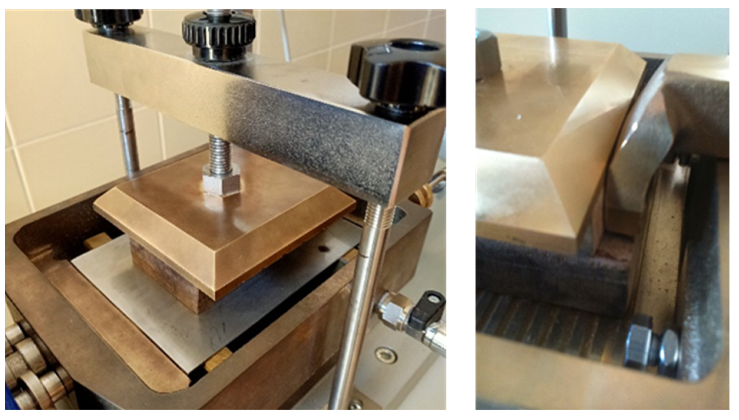
2.1. Test Implementation
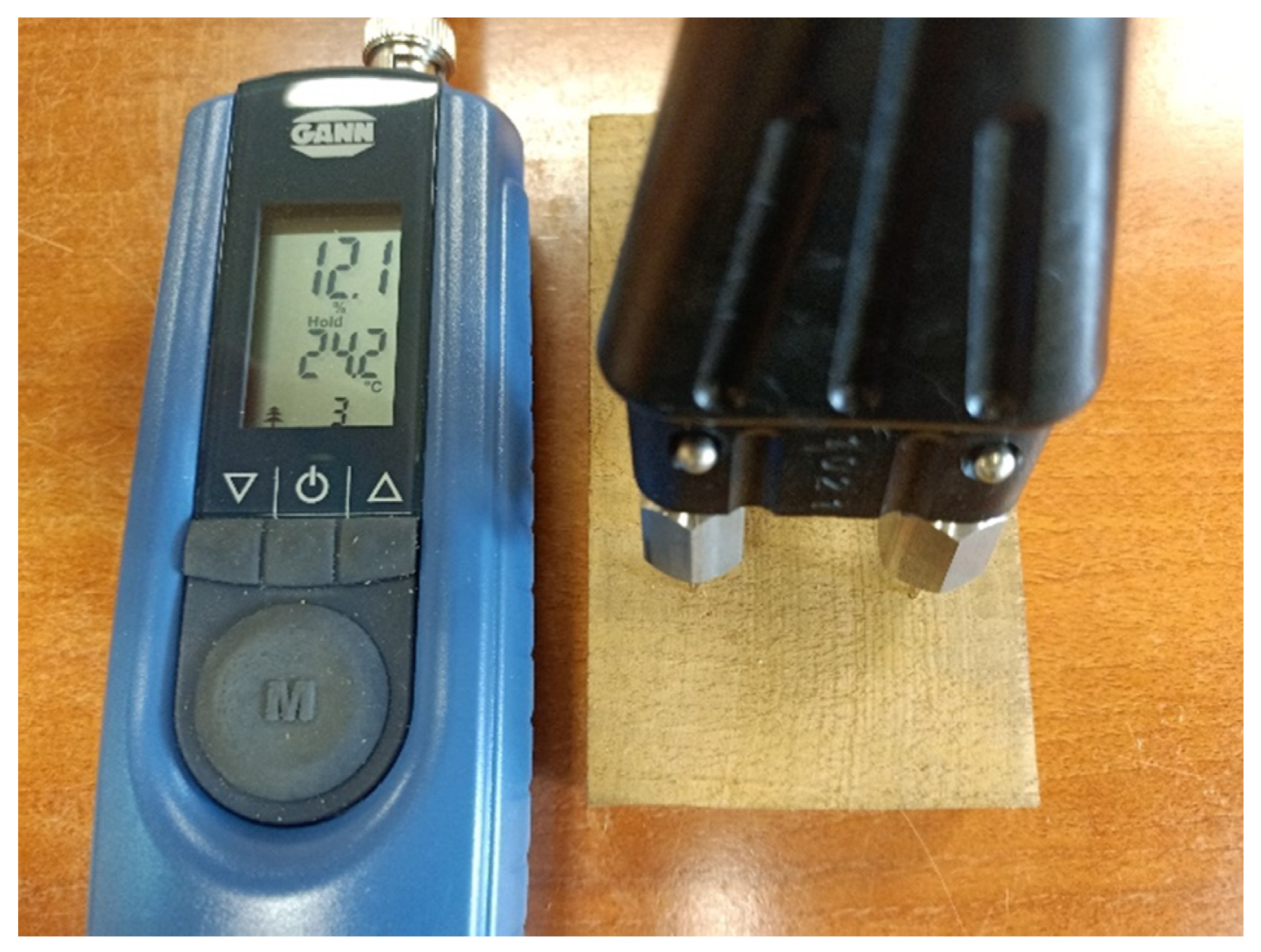
Currently, there are no European regulations regarding the performance of friction tests. Meanwhile, the American standard ASTM G-115-10 [46] includes generic recommendations to faithfully reproduce the real conditions through the experimental tests.
The methods used in this research have been extensively described in a previous work carried out by the authors [35], so only a brief description is reproduced herein to facilitate the understanding of the following sections in this manuscript.
To carry out the tests, suitably modified direct shear equipment [47] has been used. The modification allows for the surfaces of the tested materials to come into contact as well as the application of a normal load (N) and the recording of the displacement and the displacement force (F), which is the required force to constrain the movement. In this manner, the friction coefficient can be obtained according to Equations (1) and (2).
In this study, the loading plate applies a 2.5 kN vertical load through the weights incorporated in the counter-balance device, which represents a pressure of 0.5 MPa. The LVDT displacement sensor registers horizontal displacement of the carriage, which moves by an actuator at a constant speed (8 mm·min−1) to avoid the appearance of inertial forces. On one hand, the selected values are a good reflection of the typical on-site conditions; on the other hand, they favor the comparisons between methods and species as the same figures were also used in other studies [28,35,40]. Finally, a load cell sensor with a 5 kN capacity records the displacement force.
Two types of tests are conducted. In the first one, two timber pieces (timber-to-timber friction pair) are brought into contact, whereas in the second one, the contact is established between a timber specimen and a steel plate (timber-to-steel friction pair) in order to analyze the friction against this material.
The friction pair (i.e., either timber-to-timber or timber-to-steel) are arranged within the box holder of the direct shear device. Figure 3 shows the implementation layout followed for the test. In addition, the application of the normal load (N) through a load bridge on the upper part of the friction pair and a resulting horizontal displacement on the box holder can also be observed in Figure 3.

2.2. Materials

The wood material employed in this study is chestnut structural sawn timber (Castanea Sativa Mill.) of Spanish origin, which is thus regulated by [4]. Samples are obtained from certified beams with a 150 × 150 mm cross-section and 3500 mm length, classified as MEF-G grade (i.e., chestnut structural wood of great dimensions). As such, specimens complied with the grade requirements in [4]: 26.8 N/mm2 average bending strength, 10,280 N/mm2 average modulus of elasticity on bending and 582 kg/m3 average density, which corresponds to D24 strength class conforming to EN 338 [48]. The testing specimens are extracted from the aforementioned beams through sawing with a conventional wood saw blade according the desired orientations in order to obtain the friction surfaces according to the LRT axes indicated in Figure 4 and Figure 5.
In the timber-to-timber tests, two pieces of equal dimensions, 105 × 50 × 25 mm, were placed in contact through their larger surfaces. These dimensions granted the correct arrangement of the specimens. In addition, the device allowed for a friction path of 20 mm, which was appropriate to capture the stabilization of the friction force needed to define the kinetic coefficient.
In the timber-to-steel friction tests, the bottom specimen was a steel plate (S235) with similar characteristics to those used in timber mechanical joints. Note that there are similarities also in terms of its finish and roughness (Ra = 0.33 μm), to account for the slight polish in the manufacturing process. The size of the steel plate was somewhat larger than the wooden specimen previously described, which was placed on top (Figure 3-left), thus allowing the sliding path.
The orthotropy of the wood causes different roughnesses when sawing the timber in different planes, so the directions of the sawn faces must be studied according to timber anisotropy. In a previous work carried out by the authors [35], the friction between planes of the same orientation was studied. However, the study only partially covers the possibility of friction encounters between pieces in timber structures. Thus, the present research includes the study of friction between pairs of sawn chestnut timber specimens with different orientations, which represent contacts that are usually observed in joints.
The timber-to-timber friction modes studied in this work can be seen in Figure 4. These arrangements could be observed in simple supports of one timber piece over another, fixed with screws, with mortise and tenon, or in confluence with mechanical joints, such as those displayed in the group of timber-to-steel friction tests.
As shown in Figure 4 and Figure 5, several friction tests between contact faces are to be regarded—A–C, A–E, B–C, B–E—by combining the sawn surfaces and the relative directions of friction between each other. Note that the following nomenclature was employed:
Transverse surface or section, perpendicular to the grain, two sliding directions:
-
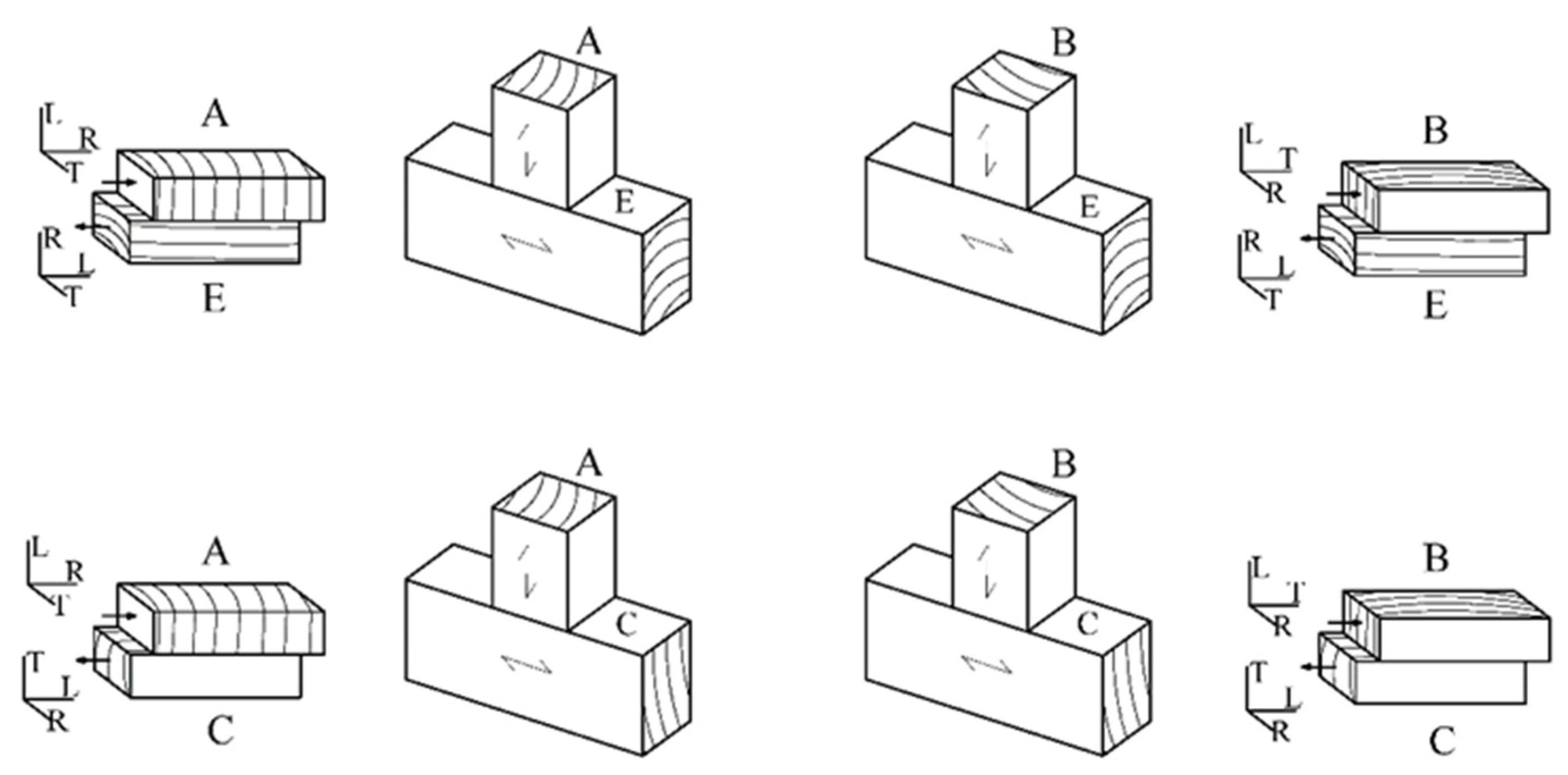
Radial sliding direction, following the radius of the annular rings, (A).
-
Tangential sliding direction, tangential to the annular rings, (B).
Radial surface or section, plane defined by the axis and the radius of the tree trunk:
-
Sliding direction parallel to the grain, (C).
-
Sliding direction perpendicular to the grain, (D).
Tangential surface or section, tangent to the annular rings:
-
Sliding direction parallel to the grain, in tangential, (E).
-
Sliding direction perpendicular to the grain, (F).
Similarly, Figure 5 displays the directions of the friction tests performed against the steel plate to reproduce the contact surfaces in mechanical joints.
As indicated in Figure 5, several friction tests—A–S, B–S, C–S, D–S, E–S, F–S—were considered. In this case, the first letter refers to the aforementioned orientations, whereas S indicates that the friction is carried against a steel plate.
From previous experiences as well as the research works conducted by other authors, it was considered that, by carrying out 15 tests in each direction, the determination of both static and dynamic friction coefficients could be ensured through a minimum of 10 values for each case.
Since the friction coefficient is affected by the moisture content (MC) of the wood, the study is carried out at the MC value corresponding to equilibrium at one of the most common work situations of structural joints, i.e., service class 1 (i.e., timber protected from damp conditions conforming to EN 1995-1-1 [49]), by considering a hygroscopic equilibrium of wood of 12%. Therefore, all friction tests, both timber-to-timber and timber-to-steel, were carried out in wood specimens conveniently conditioned at 12% MC.
According to EN 408 [50], the sample preparation was achieved at 20 ± 2 °C and 65 ± 5% humidity, which is recognized to correlate to approximately 12% MC [44], by means of a climatic chamber (MPcontrols with a temperature range of −20 °C to +60 °C ± 0.75 °C and 15 to 95 ± 2.5%). To ensure the samples reached the desired MC, several specimens were subjected to a moisture determination by the oven dry method (103 ± 2 °C) conforming to EN 13183-1 [51]. Constant mass was ascertained through successive weighings at 6 h intervals with a KERN precision scale (0.01 g) until differences were lower than 0.1%.
Nonetheless, a moisture control verification was also conducted prior to each test (Figure 6) by means of an electronic wood moisture meter (GANN- BL HT 70 with a measure range up to 70 ± 0.5%) according to EN 13183-1 [52]. Finally, after performing each friction test, a new oven drying determination was carried out to disregard any undesired MC influence.

3. Results and Discussion

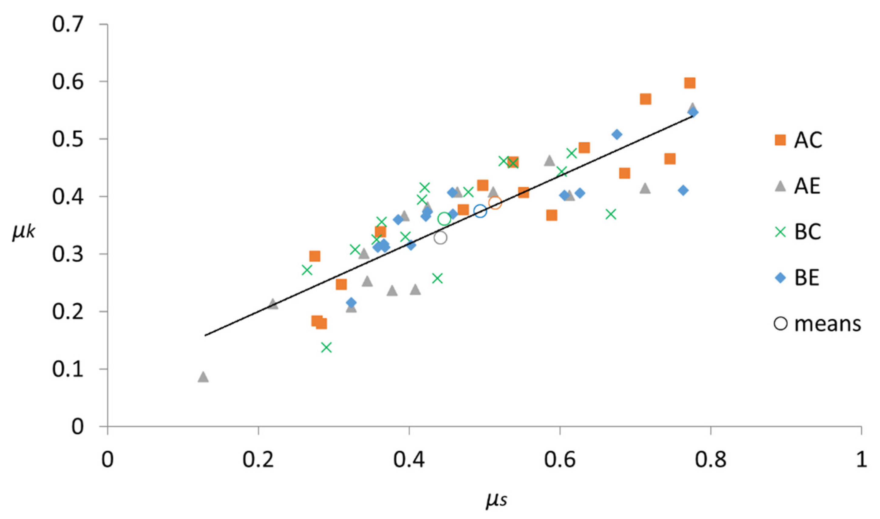
3.1. Timber-to-Timber Friction Tests

Figure 7 plots the variation of the friction coefficient versus the displacement of some representative examples for each of the different tests carried out, i.e., different orientations of the surfaces and sliding directions of friction (A–C, A–E, B–C, B–E, as stated in the previous section).
The curves plotted in Figure 7 show the typical behavior of friction between solids. Similar patterns have been also observed in a previous work [35], as well as by other authors [28,40]. The static region is distinguishable until the peak of “imminent displacement” is reached. This point constitutes the maximum value of the coefficient, and it is associated with the static value (μs). Once this maximum is reached, a decrease is noticed followed by a horizontal stabilization at the value of kinetic friction (μk). In this dynamic range, a cyclical increase and decrease in the friction force is observed as the sliding occurs. This behavior, which is known as “stick–slip”, is a frequent occurrence in timber. For instance, Möhler et al. [53], who reported three possibilities of load/slip behavior during the test, observed a similar pattern as those in Figure 7, corresponding to the presence of “stick–slip” performance. In this case, the load transfer is intermittent; the maximum load is followed by a sudden fall until the friction surface seizes again. However, despite the oscillation, the value of the initial load is no longer reached. In any case, such development of the friction measurements does not prevent the determination of the kinetic coefficient. As mentioned by several authors [41,54], the static coefficient corresponds to the upper part of the oscillations, whereas the dynamic coefficient can be ascertained from the lower part of the fluctuating curve. Table 2 shows the results obtained for the different combinations of sections and sliding directions at an average 12% MC.
From the values listed in Table 2, it can be verified that the coefficients of friction are on the same order of magnitude as those obtained in friction pairs exhibiting surfaces with the same orientation for both specimens, which are published in the authors’ previous work [35]. Nevertheless, a slight increase has been appreciated regarding the static coefficient. At an average of 0.47, it represents an approximately 5% average surge, but it is more significant for cases A–C and B–E, reaching differences up to 10%. It is also worth noting that there is no direct relationship between the highest values obtained in this investigation and those from the highest values originating from the friction pairs with the same orientations (i.e., A–A, B–B, etc.) collected in [35].
In this regard, the increase in friction between surfaces with the same orientation is greater for the dynamic friction, with an average value of 0.36, thus leading to an increase of 13%. Cases A–C and B–E reported slightly higher values, although both cases are perpendicular encounters between grain directions. It should be noted that, in these two cases, the orientation of the growth rings is also perpendicular to each other (Figure 4), which could increase friction.
Regarding the coefficients of variation, an oscillation between 27.3% and 39.7% is noticeable for the static coefficient and between 21.6% and 37% for the dynamic coefficient. Nonetheless, the reported values are similar to those obtained for friction pairs with the same orientation and those found in [28,40]. This occurrence is typical of the anisotropy of the wood and its natural variable nature [44].
The set of values obtained was within the general range of values reported for timber in the literature, as indicated in Section 1. Nonetheless, the limited number of scientific studies focusing on a specific sliding direction should be noted and, even more so, research works contemplating combining directions of friction. Thus, the results are hardly comparable more specifically than as previously indicated.
For dry spruce, Koch et al. [24] reported a static coefficient of 0.45 in friction pairs comprised of cuts perpendicular to the grain sliding against cuts at 45° to the grain. Moreover, they observed a 0.4 static friction coefficient in friction pairs comprising cuts at 45° to the grain sliding against cuts parallel to the grain. Those situations could be considered close to the ones tested here (Figure 4) and, as such, yielded similar values to those obtained in the present investigation.
For parallel to perpendicular surface encounters in oak wood, Kollman et al. [39] obtained a static coefficient of friction of 0.43 and a kinetic coefficient of 0.19. Meanwhile, the static value is comparable, and the kinetic value is significantly lower compared to the findings in this work.
For beech wood at 11.25% MC, Fu et al. [41] reported static and kinetic coefficients of 0.51 and 0.36 for tangential sections and static and kinetic coefficients of 0.43 and 0.26 for radial sections, both sliding against cross-sections. The described situations could be assimilated to the friction couples A–E and B–E for the former case and A–C and B–C for the latter. Nevertheless, note that the sliding direction in the cross section is diagonal in this work, i.e., intermediate between A and B. In any case, the obtained values are similar in both investigations, especially for both coefficients in the B–E case (0.49–0.51; 0.37–0.36), the static coefficient in the B–C case (0.45–0.43) and the kinetic coefficient in the A–E case (0.33–0.36).
Finally, the results of Xu et al. [42] are not directly comparable since the friction directions and sections are not the same as those tested in this work. However, although the surfaces were sanded with different grains, the values are on the same order as those obtained in this work.

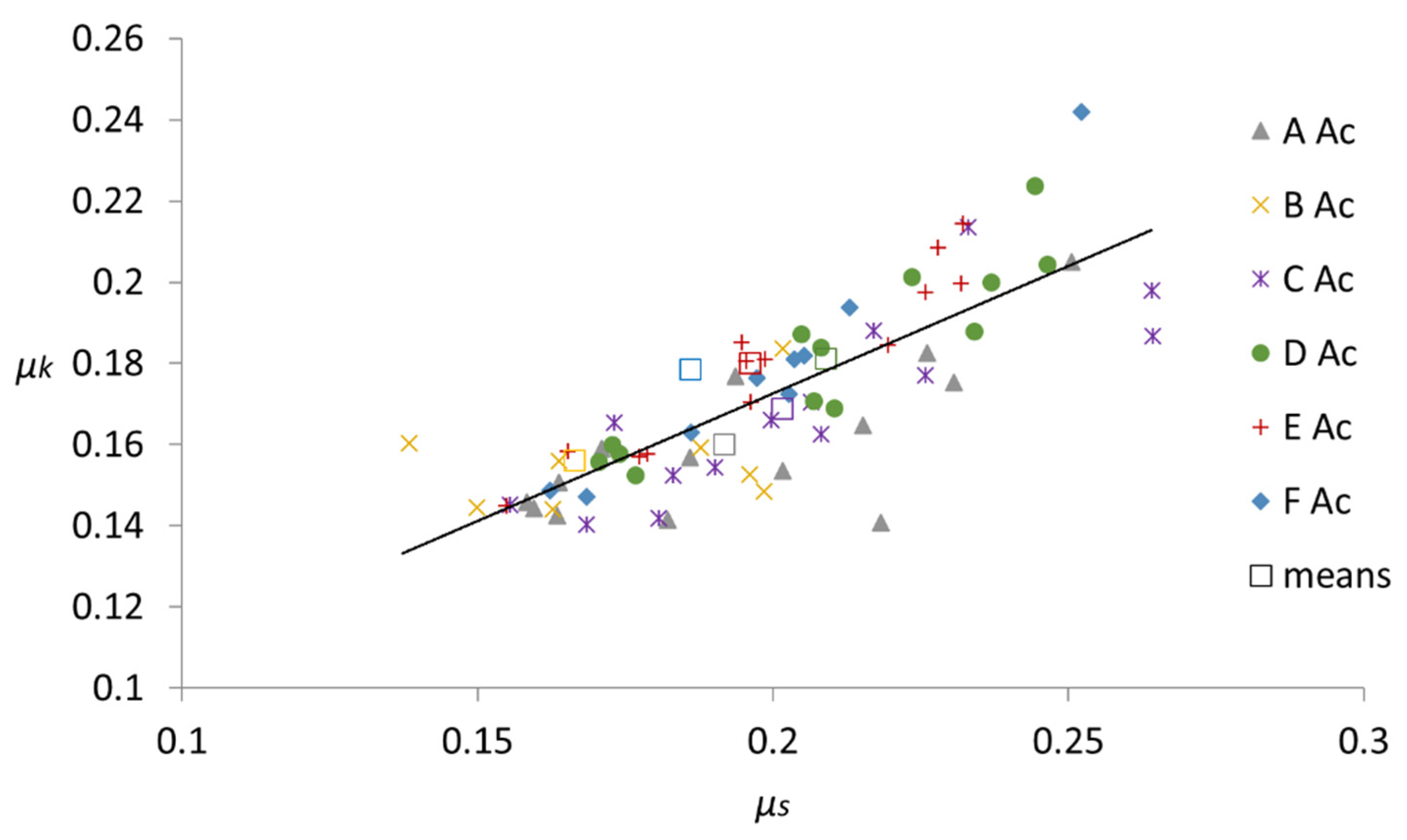
3.2. Timber-to-Steel Friction Tests

Figure 8 shows some representative curves of the friction coefficient versus displacement for each combination, i.e., section and friction direction between the timber specimen and the steel plate.
All the curves in Figure 8 show a clear transition from the static to the dynamic region. Conversely to the development observed for the timber-to-timber pairs, there is no decrease in the coefficient at the beginning of the movement, or, if it does occur, it is of no significance. However, as can be seen in Table 3, the kinetic coefficient is lower compared to the static one. As the stick–slip phenomenon is also present, the static friction is taken from the higher value of the oscillations regardless of whether it is more pronounced at the beginning of the slip, and the dynamic friction is obtained from the lower value. Fu et al. [41] clearly states this interpretation and graphically reflects this way of determining the value of both coefficients. The same interpretation is made by other authors [53,54].
Table 3 lists the average values and the coefficient of variation for the static and kinetic friction coefficients observed in the timber-to-steel tests at 12% MC. Note that, for some cases, it was not possible to clearly identify the value of the dynamic friction coefficient due to the erratic behavior of the μk—displacement plot, and so it could not be provided.
Firstly, it is worth highlighting the small difference between the static and dynamic values, at around 10%–15%. In only one case, the μk/μs ratio reaches 0.96 as a result of the aforementioned absence of an abrupt decrease in the force required at the beginning of the slide. Likewise, a reduction in the coefficients of friction can be seen compared to the previous timber-to-timber tests as the steel favors sliding with respect to the contact between wood specimens. In addition, the reduction in the coefficient of variation for each set could be attributed to the lower variability achieved by the homogeneity of one of the surfaces in contact: the steel plate. A global mean value of μs = 0.19 is obtained. It should be noted that the highest variation within a set of data was noticed for F–S, though the differences are not significant. For the kinetic friction coefficient, the mean value is 0.17 with a similar pattern in variation, as F-S shows the highest value.
The observed values are in the middle range of those reported by Dorn et al. [26], who tested Picea abies micro-laminated timber against steel. Bearing in mind that micro-laminated timber’s properties are different from those of sawn timber, the reported values for the static coefficient at 12% MC are between 0.10 and 0.30, which can be attributed to the influence of the grain angle and is in agreement with the findings of this manuscript. Although they observed a moderate influence, slight increases were reported when the sliding occurred perpendicular to the timber grain.
In any case, the observed values are lower than those suggested by the USDA Forest Products Laboratory [44] for smooth dry wood, who indicated coefficients of kinetic friction varying from 0.3 to 0.5. It should be noted that the authors differentiate between tests against hard and smooth surfaces, but there is no clear mention of steel, which could be regarded as a smooth surface. Finally, the values obtained for the coefficient of kinetic friction are in the upper range of those reported by McMillin et al. [43] and McKenzie et al. [38].

3.3. Correlation between μs and μk

Figure 9 shows the relationships between μs and μk for the set of tests carried out on timber-to-timber friction pairs, as well as the mean value for each friction combination. The mean values for the μk/μs ratio were 0.76 for the AC pair, 0.75 for the AE pair, 0.81 for the BC pair and 0.76 for the BE pair, with an overall mean of 0.77. These values are within a reduction of the dynamic coefficient around 20%–25% for common materials [33,34]. A similar behavior was observed in the previous work carried out by the authors [35] as well as in the one conducted by Fu et al. [41], who reported a mean ratio of 0.81 at 11.25% moisture content.
Furthermore, a correlation including the whole set of values leads to the linear relationship shown in Equation (3):
μk = 0.58 μs + 0.09
This correlation is similar to that obtained for friction pairs at the same orientation in a previous work [35]. Nonetheless, a lower R2 (0.74) was found due to the combination of orthotropic sections pairs. However, if each combination is considered separately, greater R2 values could be achieved, such as in the AC friction pair (μk = 0.63 μs + 0.06; R2 = 0.83), which would allow for the estimation of the dynamic coefficient once the static one is known or vice versa.
Likewise, Figure 10 shows the relationships between μs and μk for the set of tests carried out on timber-to-steel pairs, as well as the average value for each combination. In this case, the mean values for the μk/μs ratio were 0.83 for the AS pair, 0.94 for the BS pair, 0.84 for the CS pair, 0.87 for the DS pair, 0.92 for the ES pair and 0.96 for the FS pair, with a global mean value of 0.89. These values illustrate what has already been seen in Figure 8 and previously commented upon in Section 3.2 regarding the absence of a “peak” before the imminent slide followed by a sudden drop in the coefficient. The correlation for all values yields the following equation:
μk = 0.65 μs + 0.04
with R2 = 0.73, which is again a relatively low correlation value, but a greater R2 can be achieved when the directions of testing are considered separately, as in ES (μk = 0.79 μs + 0.02; R2 = 0.91) or FS (μk = 1.06 μs − 0.03; R2 = 0.96).

4. Patents

To carry out the tests in this research work, the authors developed a device that can be coupled to a direct shear equipment in order to allow for the arrangement and the friction testing between solid bodies [47].

5. Conclusions

For timber-to-timber friction pairs, the values of both the static and kinetic friction coefficients are higher when surfaces of different orientations slide against each other compared to those resulting from friction tests carried out in the same orientation. This increase is, on average, around 5% for the static coefficient and 13% for the kinetic coefficient. Moreover, the values obtained for the different combinations studied present no significant variation among themselves.
Regarding the friction tests between timber and steel, a higher value of the coefficient is not appreciated at the beginning of the slip. They presented a “stick–slip” oscillating behavior whose higher values mark the static friction coefficient, and the lower ones correspond to the kinetic coefficient. In this case, the differences between the static and dynamic values are appreciably reduced.
The coefficients of variation in the timber-to-steel test sets are reduced almost to half of those observed for the friction between pieces of timber. The lower variability included by one of the pieces, i.e., the steel plate, which is much more homogeneous, could be regarded as responsible for the differences. It was also noticed that the values obtained reflect a lower incidence of the orientation and direction of sliding in timber-to-steel pairs.
In general, the values obtained for chestnut are similar to those of other sawn timber, both in terms of friction between pieces of wood or wood against steel. However, for the latter, the scarcity of studies further limits comparison.
The friction coefficient values obtained herein could be used for the numerical simulation of joints in wooden structures by selecting those which better represent the sections, directions and materials observed in the joint to be simulated.

Author Contributions

Conceptualization, J.R.V.-G.; methodology, J.R.V.-G.; validation, J.R.V.-G., P.V.-L., D.R.-R. and M.M.I.; formal analysis, J.R.V.-G., P.V.-L., D.R.-R. and M.M.I.; investigation, J.R.V.-G., P.V.-L., D.R.-R. and M.M.I.; resources, J.R.V.-G., P.V.-L., D.R.-R. and M.M.I.; writing—original draft preparation, J.R.V.-G.; writing—review and editing, J.R.V.-G., P.V.-L., D.R.-R. and M.M.I.; supervision, J.R.V.-G. and P.V.-L.; funding acquisition, J.R.V.-G., P.V.-L., D.R.-R. and M.M.I. All authors have read and agreed to the published version of the manuscript.

Funding

This publication has been made possible thanks to funding granted by the Consejería de Economía, Ciencia y Agenda Digital of the Junta de Extremadura and by the European Regional Development Fund of the European Union through grants GR21163 and GR21091.

Institutional Review Board Statement

Not applicable.

Informed Consent Statement

Not applicable.

Data Availability Statement

Not applicable.

Acknowledgments

Administrative and technical support from Forest Research Group and Mechanical and Fluid Engineering Research Group, University of Extremadura, is gratefully acknowledged.

Conflicts of Interest

The authors declare no conflict of interest.

References

  1. Thaler, N.; Žlahtič, M.; Humar, M. Performance of Recent and Old Sweet Chestnut (Castanea Sativa) Wood. Int. Biodeterior. Biodegrad. 2014, 94, 141–145. [Google Scholar] [CrossRef]
  2. Topaloglu, E.; Ustaomer, D.; Ozturk, M.; Pesman, E. Changes in Wood Properties of Chestnut Wood Structural Elements with Natural Aging. Maderas. Cienc. Tecnol. 2021, 23, 1–12. [Google Scholar] [CrossRef]
  3. Carbone, F.; Moroni, S.; Mattioli, W.; Mazzocchi, F.; Romagnoli, M.; Portoghesi, L. Competitiveness and Competitive Advantages of Chestnut Timber Laminated Products. Ann. For. Sci. 2020, 77, 51. [Google Scholar] [CrossRef]
  4. UNE 56546; Visual Grading for Structural Sawn Timber. Hardwood Timber. AENOR: Madrid, Spain, 2013.
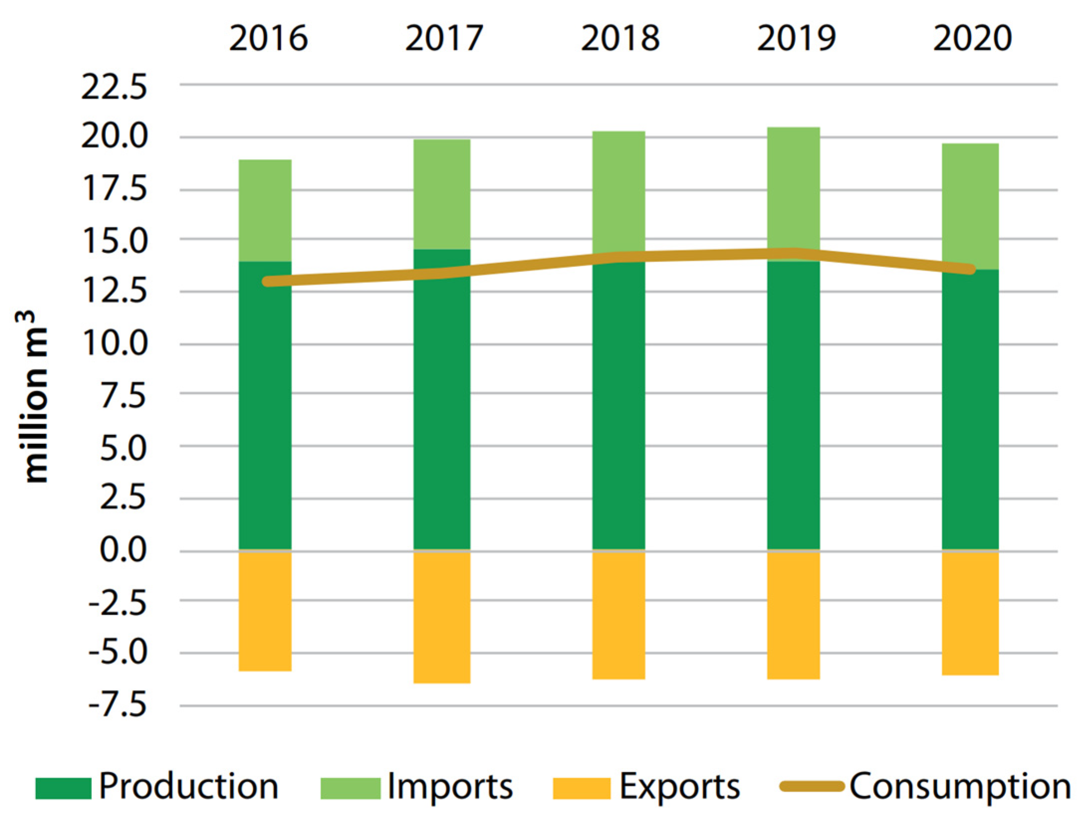
  5. FAO; UNECE. Forest Products-Annual Market Review 2020–2021; United Nations Economic Commission for Europe: Geneva, Switzerland, 2021; ISBN 978-92-1-117279-9. [Google Scholar]
  6. Conedera, M.; Manetti, M.C.; Giudici, F.; Amorini, E. Distribution and Economic Potential of the Sweet Chestnut (Castanea Sativa Mill.) in Europe. Ecol. Mediterr. 2004, 30, 179–193. [Google Scholar] [CrossRef]
  7. Ministerio para la Transición Ecológica y el Reto Demográfico. In Informe Sobre El Estado Del Patrimonio Natural y de La Biodiversidad En España a 2020; Ministerio para la Transición Ecológica y el Reto Demográfico (MITECO): Madrid, Spain, 2021.
  8. Caudullo, G.; Welk, E.; San-Miguel-Ayanz, J. Chorological Maps for the Main European Woody Species. Data Brief 2017, 12, 662–666. [Google Scholar] [CrossRef] [PubMed]
  9. Beccaro, G.; Alma, A.; Bounous, G.; Gomes-Laranjo, J. (Eds.) The Chestnut Handbook: Crop & Forest Management; CRC Press: Boca Raton, FL, USA; London, UK; New York, NY, USA, 2020; ISBN 978-0-429-44560-6. [Google Scholar]
  10. Feio, A.O.; Lourenço, P.B.; Machado, J.S. Non-Destructive Evaluation of the Mechanical Behavior of Chestnut Wood in Tension and Compression Parallel to Grain. Int. J. Archit. Herit. 2007, 1, 272–292. [Google Scholar] [CrossRef] [Green Version]
  11. Mancini, M.; Leoni, E.; Nocetti, M.; Urbinati, C.; Duca, D.; Brunetti, M.; Toscano, G. Near Infrared Spectroscopy for Assessing Mechanical Properties of Castanea Sativa Wood Samples. J. Agric. Eng. 2019, 50, 191–197. [Google Scholar] [CrossRef]
  12. Vega, A.; Dieste, A.; Guaita, M.; Majada, J.; Baño, V. Modelling of the Mechanical Properties of Castanea Sativa Mill. Structural Timber by a Combination of Non-Destructive Variables and Visual Grading Parameters. Eur. J. Wood Prod. 2012, 70, 839–844. [Google Scholar] [CrossRef]
  13. Faggiano, B.; Grippa, M.R.; Marzo, A.; Mazzolani, F.M. Experimental Study for Non-Destructive Mechanical Evaluation of Ancient Chestnut Timber. J. Civil Struct. Health Monit. 2011, 1, 103–112. [Google Scholar] [CrossRef]
  14. Vega, A.; González, L.; Fernández, I.; González, P. Grading and Mechanical Characterization of Small-Diameter Round Chestnut (Castanea Sativa Mill.) Timber from Thinning Operations. Wood Mater. Sci. Eng. 2019, 14, 81–87. [Google Scholar] [CrossRef]
  15. Ay, N.; Şahin, H. Some Mechanical Properties of Chestnut (Castanea Sativa, Mill.) Wood Obtained from Maçka-Çatak Region. Artvin Çoruh Üniversitesi Orman Fakültesi Derg. 2011, 3, 87–95. [Google Scholar]
  16. Clair, B.; Ruelle, J.; Thibaut, B. Relationship Between Growth Stress, Mechanical-Physical Properties and Proportion of Fibre with Gelatinous Layer in Chestnut (Castanea Sativa Mill.). Holzforschung 2003, 57, 189–195. [Google Scholar] [CrossRef]
  17. Marini, F.; Manetti, M.C.; Corona, P.; Portoghesi, L.; Vinciguerra, V.; Tamantini, S.; Kuzminsky, E.; Zikeli, F.; Romagnoli, M. Influence of Forest Stand Characteristics on Physical, Mechanical Properties and Chemistry of Chestnut Wood. Sci. Rep. 2021, 11, 1549. [Google Scholar] [CrossRef] [PubMed]
  18. Tamantini, S.; Bergamasco, S.; Portoghesi, L.; Vettraino, A.M.; Zikeli, F.; Mugnozza, G.S.; Romagnoli, M. Detection, Description, and Technological Properties of Colour Aberration in Wood of Standards and Shoots from a Chestnut (Castanea Sativa Mill.) Coppice Stand. Eur. J. Forest Res. 2022, 1–16. [Google Scholar] [CrossRef]
  19. EN 350; Durability of Wood and Wood-Based Products—Testing and Classification of the Durability to Biological Agents of Wood and Wood-Based Materials. CEN: Brussels, Belgium, 2016.
  20. Villar, J.R.; Guaita, M.; Vidal, P.; Arriaga, F. Analysis of the Stress State at the Cogging Joint in Timber Structures. Biosyst. Eng. 2007, 96, 79–90. [Google Scholar] [CrossRef]
  21. Villar-García, J.R.; Crespo, J.; Moya, M.; Guaita, M. Experimental and Numerical Studies of the Stress State at the Reverse Step Joint in Heavy Timber Trusses. Mater. Struct. 2018, 51, 17. [Google Scholar] [CrossRef]
  22. Villar, J.R.; Guaita, M.; Vidal, P.; Argüelles, R. Numerical Simulation of Framed Joints in Sawn-Timber Roof Trusses. Span. J. Agric. Res. 2008, 6, 508–520. [Google Scholar] [CrossRef] [Green Version]
  23. Aira, J.R.; Íñiguez-González, G.; Guaita, M.; Arriaga, F. Load Carrying Capacity of Halved and Tabled Tenoned Timber Scarf Joint. Mater. Struct. 2016, 49, 5343–5355. [Google Scholar] [CrossRef]
  24. Koch, H.; Eisenhut, L.; Seim, W. Multi-Mode Failure of Form-Fitting Timber Connections—Experimental and Numerical Studies on the Tapered Tenon Joint. Eng. Struct. 2013, 48, 727–738. [Google Scholar] [CrossRef]
  25. Villar-García, J.R.; Vidal-López, P.; Crespo, J.; Guaita, M. Analysis of the Stress State at the Double-Step Joint in Heavy Timber Structures. Mater. Construcción 2019, 69, 196e. [Google Scholar] [CrossRef] [Green Version]
  26. Dorn, M.; Habrova, K.; Koubek, R.; Serrano, E. Determination of Coefficients of Friction for Laminated Veneer Lumber on Steel under High Pressure Loads. Friction 2021, 9, 367–379. [Google Scholar] [CrossRef]
  27. Sjodin, J.; Serrano, E.; Enquist, B. An Experimental and Numerical Study of the Effect of Friction in Single Dowel Joints. Holz Als Roh-Und Werkst. 2008, 66, 363–372. [Google Scholar] [CrossRef]
  28. Crespo, J.; Regueira, R.; Soilan, A.; Díez, M.R.; Guaita, M. Methodology to Determine the Coefficients of Both Static and Dynamic Friction Apply to Different Species of Wood. In Proceeding of the 1st Ibero-Latin American Congress on Wood in Construction. CIMAD, Coimbra, Portugal, 11 June 2011. [Google Scholar]
  29. Hu, W.; Liu, N. Numerical and Optimal Study on Bending Moment Capacity and Stiffness of Mortise-and-Tenon Joint for Wood Products. Forests 2020, 11, 501. [Google Scholar] [CrossRef]
  30. Wilkinson, G.; Augarde, C. A Serviceability Investigation of Dowel-Type Timber Connections Featuring Single Softwood Dowels. Eng. Struct. 2022, 260, 114210. [Google Scholar] [CrossRef]
  31. Li, G.; Liu, Z.; Tang, W.; He, D.; Shan, W. Experimental and Numerical Study on the Flexural Performance of Assembled Steel-Wood Composite Slab. Sustainability 2021, 13, 3814. [Google Scholar] [CrossRef]
  32. Friedrich, K.; Akpan, E.I.; Wetzel, B. On the Tribological Properties of Extremely Different Wood Materials. Eur. J. Wood Wood Prod. 2021, 79, 977–988. [Google Scholar] [CrossRef]
  33. Tipler, P.A. Physics for Scientists and Engineers, 6th ed.; W.H. Freeman: New York, NY, USA, 2008; ISBN 9781429202657/1429202653. [Google Scholar]
  34. Serway, R.A.; Jewett, J.W. Physics for Scientists and Engineers with Modern Physics; Cengage Learning: New York, NY, USA, 2013; ISBN 9781133954057. [Google Scholar]
  35. Villar-García, J.R.; Vidal-López, P.; Corbacho, A.J.; Moya, M. Determination of the Friction Coefficients of Chestnut (Castanea Sativa Mill.) Sawn Timber. Int. Agrophysics 2020, 34, 65–77. [Google Scholar] [CrossRef]
  36. CEN EN 1995-2:2016; Eurocode 5: Design of Timber Structures—Part. 2. Bridges. European Committee for Standardisation: Brussels, Belgium, 2016.
  37. Argüelles, R.; Arriaga, F.; Esteban, M.; Iñíguez, G.; Argüelles Bustillo, R. Timber Structures. Joints; AITIM; Technical Research Association of the Wood and Cork Industries: Madrid, Spain, 2015; ISBN 9788487381485. (In Spanish) [Google Scholar]
  38. McKenzie, W.M.; Karpovich, H. The Frictional Behaviour of Wood. Wood Sci. Technol. 1968, 2, 139–152. [Google Scholar] [CrossRef]
  39. Kollmann, F. Wood Technology and Its Applications. Technologie Des Loses Und Der Holzwerkstoffe; Instituto Forestal de Investigaciones y experiencias y servicio de la madera; Ministerio de Agricultura: Madrid, Spain, 1959. [Google Scholar]
  40. Aira, J.R.; Arriaga, F.; Iniguez-Gonzalez, G.; Crespo, J. Static and Kinetic Friction Coefficients of Scots Pine (Pinus Sylvestris L.), Parallel and Perpendicular to Grain Direction. Mater. De Constr. 2014, 64, e030. [Google Scholar] [CrossRef] [Green Version]
  41. Fu, W.; Guan, H.; Chen, B. Investigation on the Influence of Moisture Content and Wood Section on the Frictional Properties of Beech Wood Surface. Tribol. Trans. 2021, 64, 830–840. [Google Scholar] [CrossRef]
  42. Xu, M.; Li, L.; Wang, M.; Luo, B. Effects of Surface Roughness and Wood Grain on the Friction Coefficient of Wooden Materials for Wood–Wood Frictional Pair. Tribol. Trans. 2014, 57, 871–878. [Google Scholar] [CrossRef]
  43. McMillin, C.W.; Lemoine, T.J.; Manwiller, F.G. Friction Coefficient of Oven-Dry Spruce Pine on Steel, as Related to Temperature and Wood Properties. Wood Fiber Sci. 1970, 197, 6–11. [Google Scholar]
  44. USDA. Forest Products Laboratory Wood Handbook: Wood as an Engineering Material. General Technical Report FPL-GTR-190; USDA: Madison, WI, USA, 2010. [Google Scholar]
  45. Seki, M.; Sugimoto, H.; Miki, T.; Kanayama, K.; Furuta, Y. Wood Friction Characteristics during Exposure to High Pressure: Influence of Wood/Metal Tool Surface Finishing Conditions. J. Wood Sci. 2013, 59, 10–16. [Google Scholar] [CrossRef]
  46. ASTM International ASTM G115-10(2018); Standard Guide for Measuring and Reporting Friction Coefficients. Am. Soc. Testing Materials: West Conshohocken, PA, USA, 2018.
  47. Villar García, J.R.; Vidal López, P.Y.; Moya Ignacio, M. Device to Perform Friction Tests between Solid Bodies. Utility Model U 201932027. 2020. Available online: https://patentscope.wipo.int/search/en/detail.jsf?docId=ES289318649 (accessed on 7 July 2022).
  48. EN 338; Structural Timber—Strength Classes. CEN: Brussels, Belgium, 2016.
  49. CEN EN 1995-1-1:2016; Eurocode 5: Design of Timber Structures—Part. 1.1 General. Common Rules and Rules for Buildings. European Committee for Standardisation: Brussels, Belgium, 2016.
  50. CEN EN 408:2011+A1 2012; Timber Structures—Structural Timber and Glued Laminated Timber—Determination of Some Physical and Mechanical Properties. European Committee for Standardization: Brussels, Belgium, 2012.
  51. EN 13183-1; Moisture Content of a Piece of Sawn Timber—Part 1: Determination by Oven Dry Method. CEN: Brussels, Belgium, 2002.
  52. EN 13183-2; Moisture Content of a Piece of Sawn Timber—Part 2: Estimation by Electrical Resistance Method. CEN: Brussels, Belgium, 2002.
  53. Mohler, K.; Herroder, W. Range of the coefficient of friction of spruce wood rough from sawing. Holz Als Roh-Und Werkst. 1979, 37, 27–32. [Google Scholar] [CrossRef]
  54. Li, L.; Gong, M.; Li, D.G. Evaluation of the Kinetic Friction Performance of Modified Wood Decking Products. Constr. Build. Mater. 2013, 40, 863–868. [Google Scholar] [CrossRef]
Figure 1. Sawn hardwood production, trade and consumption in Europe (exports are shown as negative numbers) [5].
Forests 13 01078 g001
Figure 2. Distribution map of Castanea sativa [8].
Forests 13 01078 g002
Figure 3. View of the layout of the timber-to-steel friction test (left) and detail of the evolution of the timber-to-timber test (right).
Forests 13 01078 g003
Figure 4. Contact modes studied in timber-to-timber joints and friction faces indicating the direction of slip (L—longitudinal direction, trunk axis; R—radial to growth rings; T—tangential to growth rings).
Forests 13 01078 g004
Figure 5. Contact modes studied in mechanical joints. Generated friction tests: (a) A–S, (b) B–S, (c) C–S, (d) D–S, (e) E–S, (f) F–S. (S—Steel plate). (L—longitudinal direction, trunk axis; R—radial to growth rings; T—tangential to growth rings).
Forests 13 01078 g005
Figure 6. Moisture content control (12%) prior to friction test.
Forests 13 01078 g006
Figure 7. Representative examples of the variation of the coefficient of friction against the displacement for the different combinations of surfaces and sliding directions: A–C; A–E; B–C; B–E.
Forests 13 01078 g007
Figure 8. Representative examples of the variation of the coefficient of friction against the displacement for the different combinations of surfaces and sliding directions against steel: A–S; B–S; C–S; D–S; E–S; F–S.
Forests 13 01078 g008
Figure 9. Relationships between the values of μk and μs for the different timber-to-timber friction pairs, as well as the mean value for each case (indicated by a circle of the referred color) and the fitted line (μk = 0.58 μs + 0.09).
Forests 13 01078 g009
Figure 10. Relationship between the values of μk and μs for the different timber-to-steel friction pairs, as well as the mean value for each case (indicated by a square of the referred color) and the fitted line (μk = 0.65 μs + 0.04).
Forests 13 01078 g010
Table 1. Properties related to engineering of defect-free chestnut timber [9].
PropertyRange
Density in green condition700–1100 kg/m3
Density at 12% MC470–700 kg/m3 (Average: 580 kg/m3)
Total linear shrinkageAxial: 0.6%
Radial:4.1%
Tangential: 6.1%
(Average volumetric: 10.8%)
T/R anisotropy ratioAround 1.5
Compression strength21–64 N/mm2 (Average: 51 N/mm2)
Bending strength50–140 N/mm2 (Average: 86 N/mm2)
Modulus of elasticity on bending8450–14,400 N/mm2 (Average: 11,380 N/mm2)
Shear strength5.7 to 9.2 N/mm2 (Average: 7.3 N/mm2)
Shock resistance and hardnessLow to medium
Durability to basidiomycetesClass 2 [19]
Durability to xylophagous insectsClass D [19]
Durability to termitesClass M [19]
TreatabilityClass 4—extremely difficult
Use class complying with natural durabilityClass 3—for external use (but not in ground contact or with permanent humidification)
Table 2. Coefficients of friction between timber surfaces at 12% MC. (CoV: coefficient of variation).
Specimen123456789101112131415Average (CoV %)
A–Cμs0.310.280.690.590.530.550.280.280.770.710.360.630.540.750.470.51 (34.6)
μk0.250.300.440.370.420.410.180.180.600.570.340.490.460.470.380.39 (32.1)
A–Eμs0.410.380.130.460.420.220.510.390.340.610.710.340.780.320.590.44 (39.7)
μk0.240.240.090.410.380.210.410.370.250.400.420.300.550.210.460.33 (37.0)
B–Cμs0.330.390.290.440.600.670.420.360.360.620.420.530.540.480.260.45 (27.3)
μk0.310.330.140.260.440.370.390.320.350.480.400.460.460.400.270.36 (25.6)
B–Eμs0.770.370.400.630.760.360.370.390.320.460.680.460.610.420.420.49 (31.0)
μk0.550.320.320.410.410.310.310.360.220.410.510.370.400.360.370.37 (21.6)
Table 3. Coefficients of friction between timber and steel surfaces depending on the orientation of the contact surfaces and the slip direction (CoV: coefficient of variation).
Specimen123456789101112131415Average (CoV %)
A-Sμs0.250.220.180.200.230.230.190.160.190.160.160.150.220.170.160.192 (16)
μk0.200.140.140.150.180.180.180.180.140.160.14-0.160.160.150.16 (11.8)
B-Sμs0.140.160.200.150.200.140.190.130.200.150.150.160.160.16-0.16 (14.0)
μk-0.140.150.140.150.160.16-0.18--0.150.160.14-0.15 (8.5)
C-Sμs0.210.180.180.150.190.160.210.170.230.260.260.220.230.170.200.20 (17.3)
μk0.170.140.15-0.150.150.160.160.210.190.200.190.180.140.170.17 (13.0)
D-Sμs0.240.240.180.250.170.210.170.200.220.200.220.230.210.210.170.21 (12.6)
μk0.200.220.150.200.160.170.160.19--0.200.190.180.170.160.18 (12.3)
E-Sμs0.230.180.230.150.180.190.200.200.220.200.230.230.200.170.150.20 (14.0)
μk0.210.160.21-0.160.190.18-0.180.180.200.200.170.160.150.18 (12.0)
F-Sμs0.190.210.170.190.130.160.200.130.250.190.210.200.190.20-0.19 (18.9)
μk0.180.190.150.16-0.150.17-0.24-0.180.180.170.18-0.18 (15.1)
Publisher’s Note: MDPI stays neutral with regard to jurisdictional claims in published maps and institutional affiliations.

