Abstract
This research aimed to develop statistical models to predict basal area increment (BAI) for Araucaria angustifolia using Artificial Neural Networks (ANNs). Tree species were measured for their biometric variables and identified at the species level. The data were subdivided into three groups: (1) intraspecific competition with A. angustifolia; (2) the first group of species that causes interspecific competition with A. angustifolia; and (3) the second group of species that causes interspecific competition with A. angustifolia. We calculated both the dependent and independent distance and the described competition indices, considering the impact of group stratification. Multi-layer Perceptron (MLP) ANN was structured for modeling. The main results were that: (i) the input variables size and competition were the most significant, allowing us to explain up to 77% of the A. angustifolia BAI variations; (ii) the spatialization of the competing trees contributed significantly to the representation of the competitive status; (iii) the separate variables for each competition group improved the performance of the models; and (iv) besides the intraspecific competition, the interspecific competition also proved to be important to consider. The ANN developed showed precision and generalization, suggesting it could describe the increment of a species common in native forests in Southern Brazil and with potential for upcoming forest management initiatives.
1. Introduction
Ecologists and foresters have sought to understand what factors influence the growth variation of plants and trees, which is essential to explaining forest productivity and dynamics [1]. Among these factors, the most important internal factors are physiology, species, age, and genetic characteristics [2,3], and the most important external factors are climatic conditions, soil-slope, type of competition, and nearby trees [4], besides natural disturbances and silvicultural cutting practices [5].
The basal area increment (BAI) has been modeled based on individual tree size, stand development, and other variables of site and competition to analyze the influence of competition and aridity on tree productivity [6]. Individual-based modeling is one of the most comprehensive and detailed approaches to predicting individual trees’ growth. It has been applied to simulate future forest management scenarios [7], predict/explain wood quality [8], predict habitat quality [9], and plan forest management activities [10].
Competition is a key process in regulating tree and stands dynamics. In mixed forests, the effect of species interactions can be assessed by quantifying the influence of intra- and inter-specific competition on tree growth. Over the years, studies [11,12,13] have reported on the competition between angiosperms and conifers primarily because angiosperms reportedly change conifers in most forest types in the tropics [13]. In mixed conifer-angiosperm forests in the Southern hemisphere, the long-term dominance relationship between conifers and angiosperms is also known as “temporal stand replacement” or Lozenge model, being reported in several studies [13,14,15].
Mixed Ombrophilous Forests (MOF) consist of a mixture of tropical and temperate floras formed by hundreds of tree species. The Brazilian Pine (Araucaria angustifolia (Bertol.) Kuntze, Araucariaceae) is characteristic and an exclusive native to MOF, being considered the most important coniferous tree of Brazil due to its high wood quality of medium density and its valued edible seeds [16,17,18]. Intensive and often indiscriminate harvesting have significantly reduced the area of the forest. A. angustifolia is protected by the law (Law RS 9519-92) and included in the red list of endangered species by the Brazilian government and the International Union for Conservation of Nature [19]. Logging of this species is therefore prohibited [17].
Several studies have been applying better statistical techniques and mathematical methods to model forest incrementation and determine the relationship between growth rates and various independent internal and external variables. These methods and techniques include both linear and non-linear regressions, fuzzy logic, Mixed Models (MM), and, more recently, Artificial Neural Networks (ANNs) [20,21,22,23]. The ANNs’ synthesis of information in a single network helps work with a large amount of data from different locations, genotypes, climatic conditions, sites, and silvicultural interventions, among other site characteristics that influence tree growth. Continuous and categorical variables can thus be used simultaneously in a single trained network to reach accurate estimates [4,24].
ANNs form a subset of artificial intelligence (AI) which are efficient alternatives to estimate tree growth [25,26,27], the prognosis of tree diameter, height, and volume [28,29,30], survival and mortality [31], biomass and carbon [32,33]—applied with remote sensing data [34,35]—as well as species richness and composition mapping [36]. ANNs are used to improve estimates in mixed forests since modeling in this type of forest is complex and must consider species interactions, long dynamics of spatial or temporal gradients in resource availability, and climatic conditions. To estimate the volume increment in the mixed-age Hyrcanian forest of irregular age in Iran, ANN and the support vector machine were better and more accurate than other machine learning methods and traditional least squares regression [28]. In Brazil, ANNs were used to estimate the biomass and volume of different species of Cerrado (Brazilian savanna), obtaining better results than the non-linear mixed effects (NLME) and Random Forest (RF) models [37]. ANN was also applied in MOF to estimate the bark thickness of Araucaria angustifolia [38], but the application of AI techniques to improve estimates of species growth in this type of forest must be further investigated. This study, therefore, aims to model BAI for Araucaria angustifolia (Bertol.) Kuntze in a mixed ombrophilous forest in Southern Brazil. Our specific objectives are to: i. separate trees in groups according to their Importance Value Index (IVI) of the trees; ii. characterize the effect of competition between groups; iii. develop models using artificial neural networks (ANNs).
2. Materials and Methods
2.1. Study Area
This research was developed at the Sustainable Use Conservation Unit in the São Francisco de Paula National Forest (FLONA-SFP) [29°25′ S and 50°23′ W]. The MOF study area occupies 902 ha (≈56%) of a total area of 1606.7 ha.
The FLONA-SFP is located about 930 m above sea level in the northeastern region of the state of Rio Grande do Sul in the municipality São Francisco de Paula. The characteristic climate is medium mesothermal (Cfb), a temperate climate with rainfall above 2000 mm evenly distributed throughout the year, and a mean annual temperature below 15 °C [39]. Table 1 gathers the definitions used in this long study.

Table 1.
Definitions of symbols and units used along this study.
2.2. Characteristics of the Forest
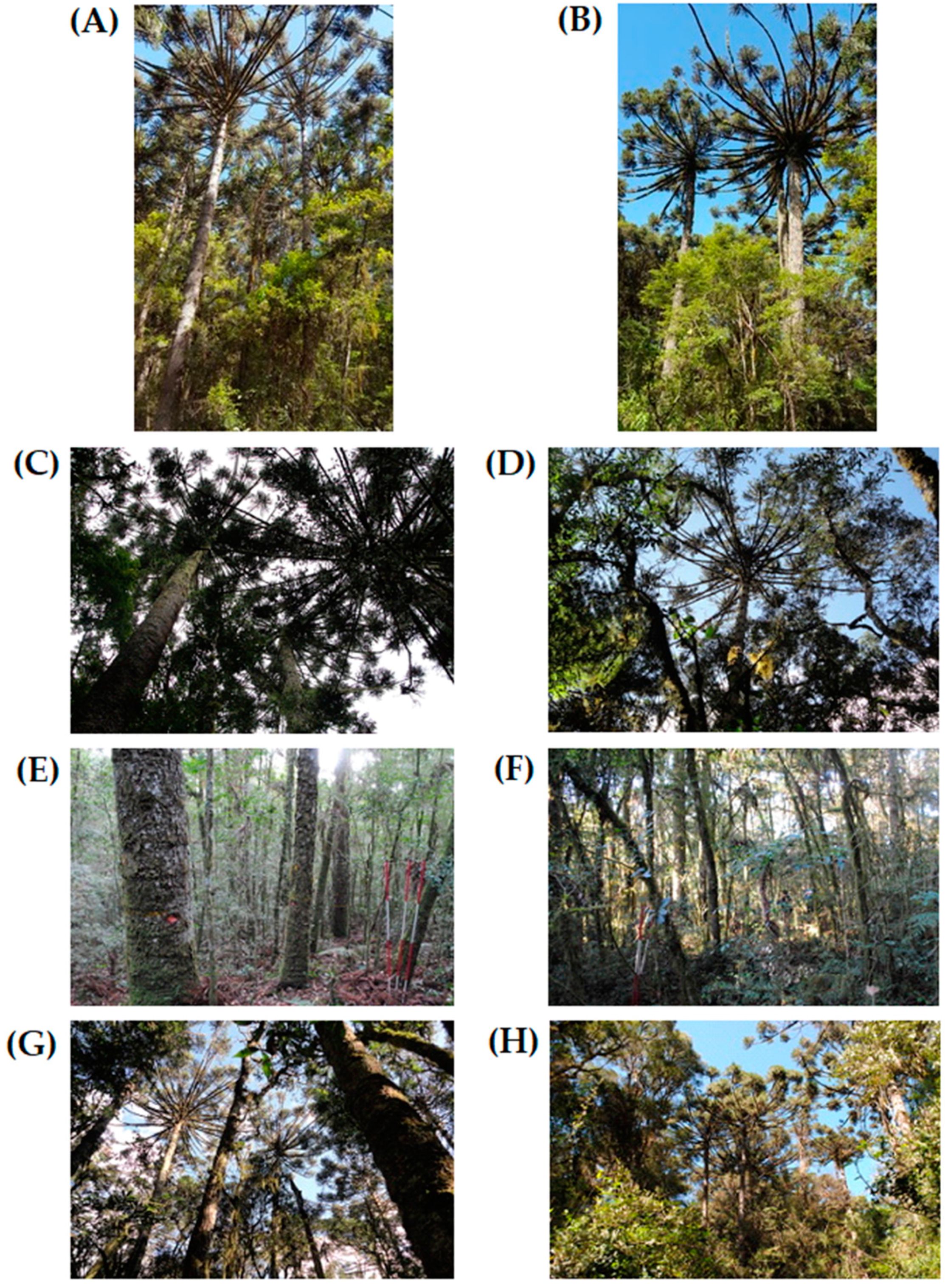
The Mixed Ombrophilous Forest (MOF) are subtropical conifer-hardwood mixed forests part of the Atlantic forest’s floristic dominion in South America. They are characterized by the presence of Araucaria angustifolia (Bertol.) Kuntze (Figure 1) [14], which are in the upper canopy of the forest and dominant in the vegetation [40]. The MOF is considered one of the most threatened phytophysiognomies in Brazil [41] since intensive and often indiscriminate harvesting in past decades have significantly reduced the original area occupied by this forest. The current legislation thus restricts forest management by prohibiting the harvest of the most important timber tree species found in this forest, including Araucaria angustifolia [42].
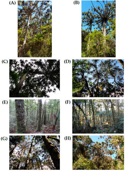
Figure 1.
Growth conditions of A. angustifolia in Mixed Ombrophilous Forest in Southern Brazil. (A) trees inside the forest; (B) trees at the edge of the forest; (C) intraspecific competition; (D) interspecific competition; (E) predominance of Brazilian pine trees within the plot; (F) predominance of other species of native trees within the plot; (G) vertical forest structure with predominant intraspecific competition; (H) vertical forest structure with predominant interspecific competition. Photos were taken by C.A.G.F.
The study site has low floristic diversity with a Shannon diversity index of 1.58 and ecological dominance of a few species with a Pielou equability index of 0.93 [43]. The A. angustifolia had an Importance Value Index (IVI) of 41.60% and 79.29% of the total basal area of the study site. The most frequent species found were Araucaria angustifolia, Casearia decandra Jacq., Blepharocalyx salicifolius (Kunth) O.Berg., Ilex brevicuspis Reissek, and Ilex paraguariensis A.St.-Hil (Table 2).

Table 2.
Dendrometric and phytosociological characterization of the species trees in plots of mixed ombrophilous forest in Southern Brazil.
2.3. Data Collection
The data were collected from the Long-Term Ecological Research (LTER), installed in 2002 and re-measured annually over eight years. This plot was selected considering the largest number of trees, the largest number of A. angustifolia, and a proper conservation stage. The development of models was considered only for the species A. angustifolia. Variables of size, site, and competition were considered for 331 A. angustifolia trees. The measurement was conducted in 25 square sample plots, with 20 m totaling one hectare (ha). Twenty plots (80%) were used for training (fitting) of the BAI models and five plots (20%) were used for validation purposes. This dataset partition was spatially idealized so that the selected trees covered the entire variability of the study area.
Firstly, we took the measured circumference at the breast height (therefore, c) and converted it to diameter at the breast height (d = c/). The total height (h) of single trees was measured using Vertex IV’s hypsometer (Haglof, Sweden). With these measurements, the Assmann dominant height (h100), the basal area per hectare (G), the number of trees per hectare (N), and the average diameter (daverage) were obtained.
The competition effect of A. angustifolia trees was assessed using competition indices proposed by Lorimer [44] (Equations (1)–(4)). In addition, the dependent distance described by Hegyi [45] was also considered (Equations (5)–(8)). Finally, the total competition of the target tree was classified according to the groups described in Table 2.
where Lorimer: competition index of Lorimer—the numerical values of the sub-indices are (1) intraspecific competition with A. angustifolia, (2) first group of species that cause interspecific competition with A. angustifolia, (3) second group of species that cause interspecific competition with A. angustifolia (see Table 2); di and dj: diameter at 1.30 m above ground level (d) of target tree i and competitor j (cm).
where Hegyi: competition index of Hegyi—the numerical values of the sub-indices are (1) intraspecific competition with A. angustifolia, (2) first group of species that cause interspecific competition with A. angustifolia, (3) second group of species that cause interspecific competition with A. angustifolia (see Table 2); di and dj: diameter at 1.30 m above ground level (d) of target tree i and competitor j (cm); distij: distance between target tree i and competitor j, in (m).
Growth rates were assessed using periodic annual basal area increments (BAI) and calculated in subsequent continuous measurements of the diameter of A. angustifolia.
where BAI: periodic annual increment in basal area (cm2.year−1); dt: diameter at breast height at the end of the period (cm); dt−2: diameter at breast height at the beginning of the period (cm); and t: period in years. * Measured in intervals of two years.
2.4. Correlation Analysis
Correlation analysis determines the degree of relationship between two variables, where the values vary between 0 and 1. Values close to 1 indicate a great correlation between the variables. Pearson’s correlation analysis Equation (10) was used to describe the level of association between BAI and variables of size, site and competitions, considering a 5% level of significance:
where : Pearson’s correlation coefficient; xi: observed value of x; : mean of the observed values x; yi: observed value of y; : mean of the observed values y; n: number of observations.
2.5. Modeling Using Artificial Neural Networks (ANNs)
Multi-layer Perceptron (MLP) ANNs with only one hidden layer were used for data training (Haykin [46]) starting from Data Normalization (DN) according to two types of intervals [0; 1] and [−1; 1], given by Equation (11):
where Xi: value to be equalized; Xminimum: lowest value of the data set; Xmaximum: highest value of the data set; UL: upper limit; and IL: inferior limit.
This equalization was used to prevent variables of greater magnitude from influencing the result more [46]. Table 3 shows the number of neurons and activation functions.

Table 3.
Configuration of artificial neural networks to describe the BAI of the A. angustifolia in mixed ombrophilous forest in Southern Brazil.
We used the activation functions (hyperbolic tangent and logistic sigmoid) of the intermediate layer and activation functions (identity) of the output. In training, the ideal number of neurons was found by the Fletcher-Gloss method [47], given by Equation (12):
where n: number of network inputs; n1: number of neurons in the hidden layer; and n2: number of neurons in the output layer.
The ANN prediction uses the mathematical Equation described for MLP [3], as follows:
where Y: estimation of the value of the dependent variable; Xi: input value of the i-th independent variable; wij: connection weight between the i-th input neuron and the j-th neuron of the hidden layer; βj: bias value of the j-th neuron of the hidden layer; vj: connection weight between the j-th neuron of the hidden layer and the output neuron; θ: bias value of the output neuron; f(.): hidden layer activation function; g(.): output activation function.
ANNs were trained according to the DN evaluated, activation functions (AF) types, and neurons in the hidden layer (NHL) variations. The maximum amount of NHL defined by the method in Equation (2) sought to avoid memorizing the input data (over-fitting) or extracting insufficient information in training (under-fitting).
2.6. Data Analyses and Statistical Criteria
All the statistical analyses were processed using the package neuralnet available inR version 3.4.4. The goodness of fit criteria used to assess model performance was based on the coefficient of determination Equation (14), root mean square error Equation (15), mean absolute error Equation (16), and mean absolute percentage error Equation (17). In addition, the graphical analysis of residue was adopted as complementary.
i. Coefficient of determination (R2)
ii. Root mean square error (RMSE)
iii. Mean absolute error (MAE)
iv. Mean absolute percentage error (MAPE)
v. and graphical analysis of residues.
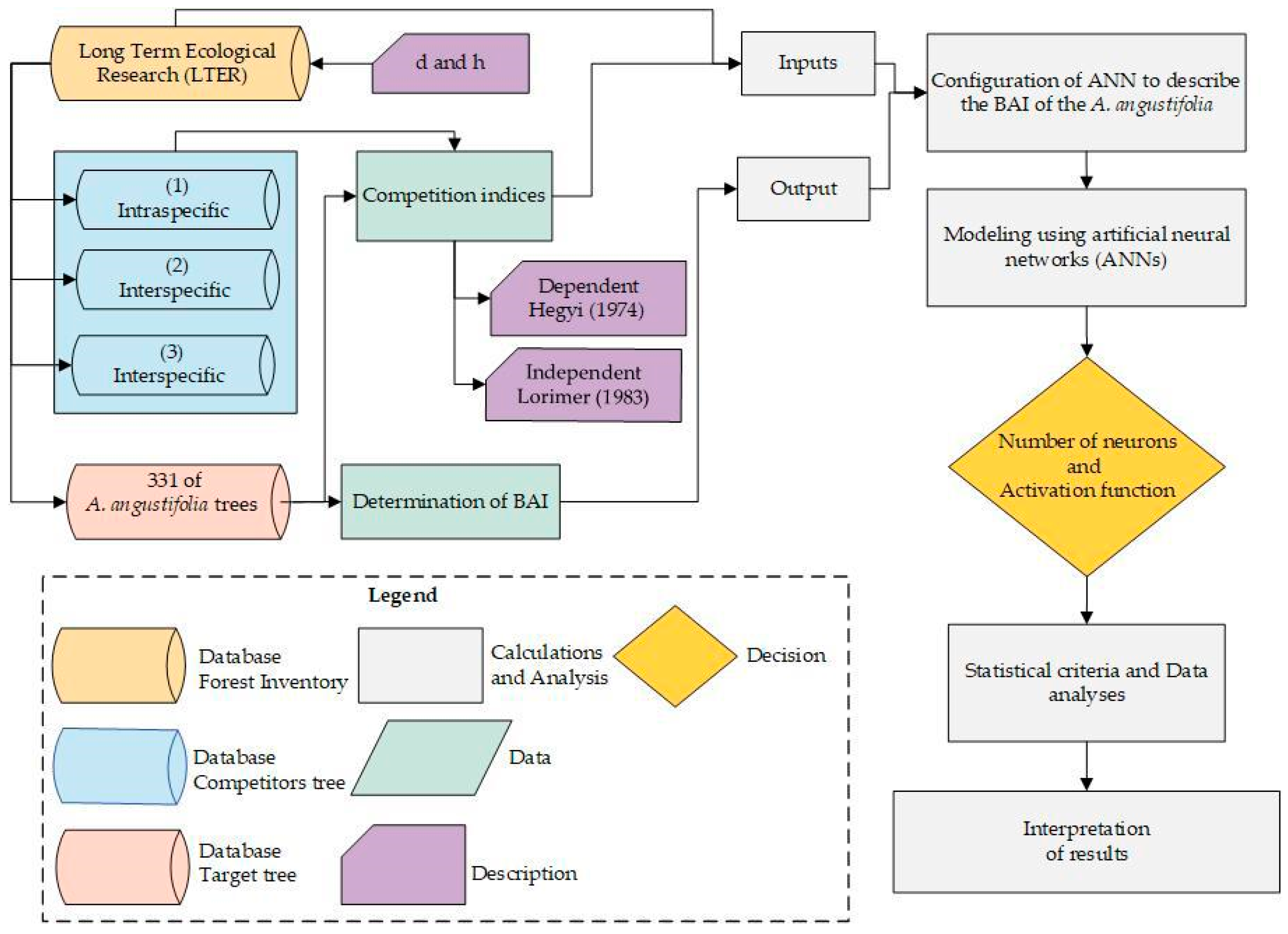
Figure 2 shows the workflow used in this study to develop the BAI model using species groups and ANN.
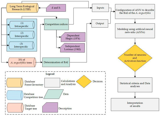
Figure 2.
Flowchart of the workflow steps adopted in this study.
3. Results
3.1. Characteristics of the Trees in the Forest
The results of the horizontal structure analysis (Table 2) emphasize, among the 48 species cataloged in the area, the ecological importance of A. angustifolia in terms of IVI in the structure of forest remnants, including the influence of intraspecific competition on the species. Together with seven other species classified as group 2 (interspecific 2; Table 2), this species represents more than 70% of the total IVI of the forest. All other species categorized as group 3 (interspecific 3; Table 2), which contains more species, had IVI values lower than 2.00.
3.2. Characteristics of the Brazilian Pine Trees in the Plots
The sampled A. angustifolia trees (n = 260 training and n = 71 validation) covered a wide range of diameter (10.0–75.3 cm) and presented a higher variability, characteristic of uneven-aged natural forests. Trees ranged from facing high levels of competition to being less influenced by their surroundings, represented by the Lorimer and Hegyi indices (Table 4). The intraspecific competition, characterized by Lorimer1 and Hegyi1, was overall higher than the interspecific competition which affects A. angustifolia trees (Lorimer2, Lorimer3; Hegyi2, Hegyi3). Tree increment averaged 9.5 cm2.year−1 and trees with growth very close to zero were also recorded. The site-specific variables (h100, G, N, and daverage) usually showed less marked variability.

Table 4.
Descriptive statistics for measured variables of A. angustifolia in a Mixed Ombrophilous Forest in Southern Brazil.
3.3. Pearson’s Correlation of BAI with Variables Describing Size, Site, and Competitions
All size and competition-tested variables were significantly correlated (p < 0.01) with BAI (Table 5). The size variables ‘diameter’ and ‘height’ stand out, representing intrinsic characteristics of the tree itself (internal factors) and its ability to withstand external factors and keep growing. Regarding the competition variables, characterized by the Lorimer and Hegyi indices, negative correlation values were verified, representing the inverse nature of the relationship.

Table 5.
Pearson’s correlation between BAI vs. variables of size, site, and competition of the A. angustifolia in a Mixed Ombrophilous Forest in Southern Brazil.
Site-representative variables, in turn, had low associations with BAI, possibly because of the lower heterogeneity identified for these variables between the studied plots—likely influenced by the contiguous design of the area.
3.4. Modeling Using Artificial Neural Networks (ANNs)
Based on the correlations obtained in the previous item, only the size and competition variables were considered for inclusion in the increment models via artificial neural networks (Table 3; Table 6). Accuracy gains in relation to the most basic model, which considered only the diameter, can be observed according to the inclusion of other variables in the networks, represented by the variations of R2, RMSEMAE, and MAPE. The analysis of variance followed by the Tukey test at 1% and 5% applied to the MAE statistic helps observe the significance of these variations (Table 6).

Table 6.
Artificial neural networks and statistics of precision and accuracy of BAI models for A. angustifolia in a Mixed Ombrophilous Forest in Southern Brazil.
Based on the structured networks, up to 77% of the A. angustifolia BAI variations could be explained. In comparison with model Id1, positive R2 variations of up to 0.36 were recovered while RMSE decreased to −2.77 and MAE decreased to −1.83. On the other hand, the Id33 model differed significantly from the model represented only in diameter only (p < 0.05; Table 6).
Regardless of the combination of variables assessed, models that combined competition indices based on Hegyi’s formulation performed better than those that included the Lorimer index. For the Hegyi models, the spatialization of the competing trees helped represent the effective influence on the central tree and understand how competition pressure affects growth.
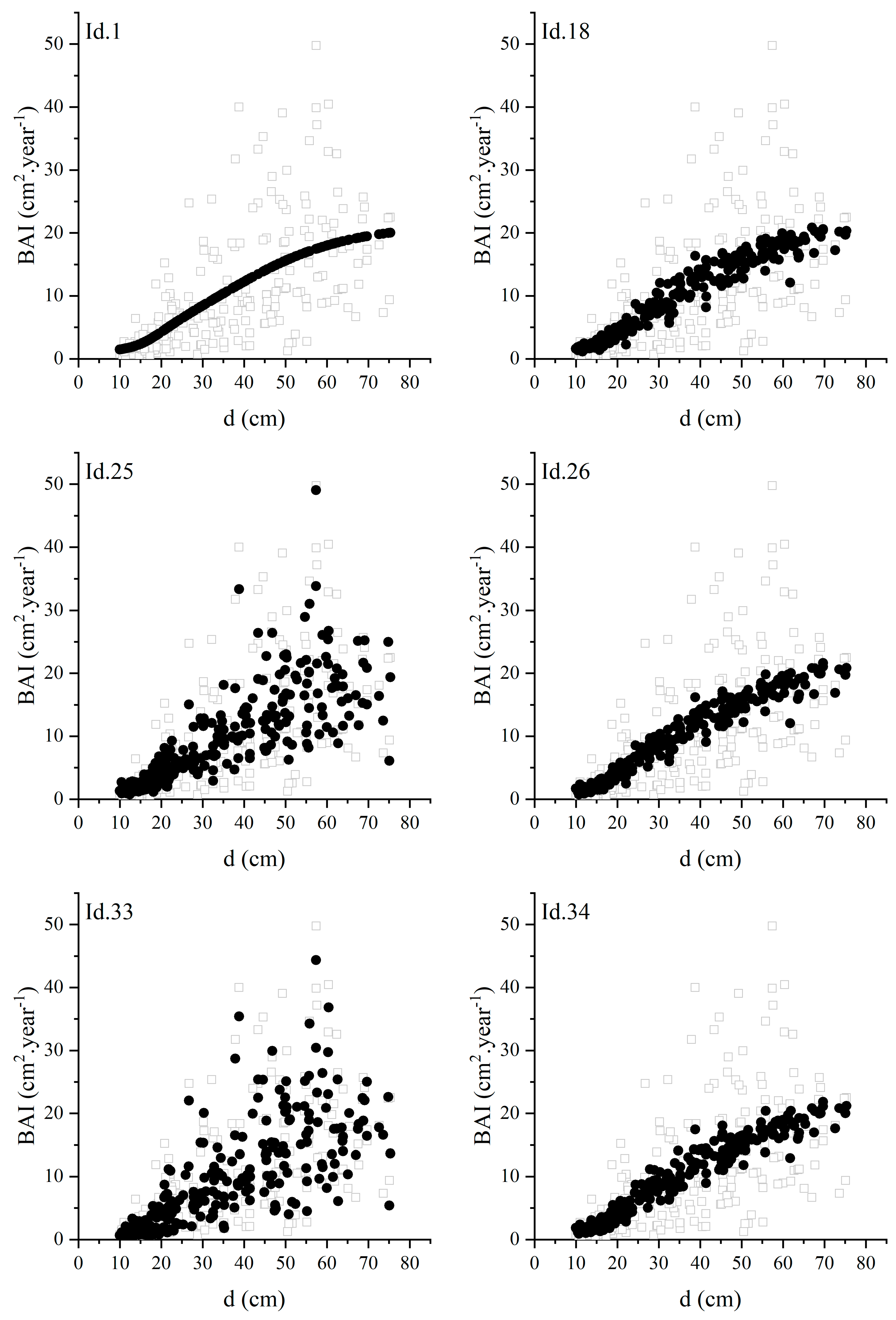
Furthermore, using separate variables for the sums of each group helped explain the BAI more than using one variable for the index including all sums, thus covering variations much better (Table 6; Figure 3). Considering the characteristics of the studied forest and the forests with A. angustifolia overall, we expected that the competition represented by Group 1 (intraspecific competition) would be more associated with growth than the competition of Groups 2 and 3 (interspecific competition), especially because of the dominance pattern of the species. This was true when only these CI variables were included separately in the model (Id2, Id3, and Id4; Id10, Id11, and Id12), with better performance of Lorimer1 and Hegyi1 (Table 6). However, when these competition indices were combined with variables d and h, the three groups (Id19, Id20, and Id21; Id27, Id28, and Id29) had very similar performance.
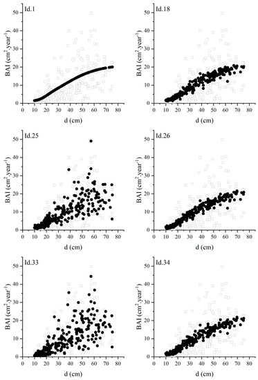
Figure 3.
Periodic annual basal area increment (BAI, cm2.year−1) predictions vs. tree diameter (d, cm) for A. angustifolia in a mixed ombrophilous forest in Southern Brazil. Please check Table 6 for a description of the model id and selected variables.
Moreover, when two distinct competition groups were included in the model, the combined competition of Group 1 and Group 3 covered the growth variations of the species more than that of Group 1 and Group 2. Figure 3 shows these characteristics of the generated models, explaining the high capacity of the networks to represent the variability found within the data set for the relationship. The Id25 and Id33 models thus stand out, reaching even the extreme points of BAI variability since their competitive contribution was observed within the three IVI groups (intra and interspecific).
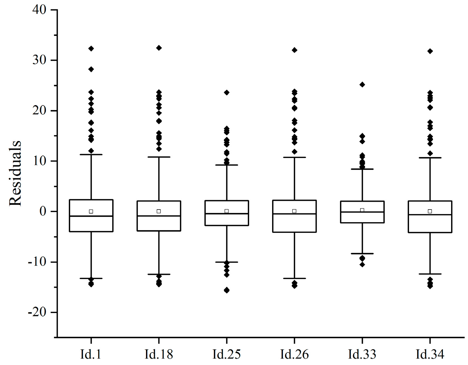
The smallest interquartile difference identified in the residual analysis for the Id33 model (Figure 4), which also considers the influence of the distance factor between objective and competitor trees, reinforces the good performance of this model in BAI modeling for Araucaria angustifolia.
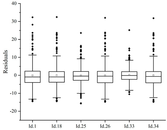
Figure 4.
Residual analysis of the trained network of the best BAI models for A. angustifolia in a mixed ombrophilous forest in Southern Brazil.
3.5. Validation of the Developed Models
All generated models performed satisfactorily in the Wilcoxon nonparametric test for validation (Table 7), considering that, at 5% probability, none of the models showed significant differences between observed and estimated values. Furthermore, the highest probability values retrieved coincided with the models that excelled in training, with no evidence of overfitting networks, thus showing the stability and potential for generalization of these models.

Table 7.
Validation of the ANNs for A. angustifolia BAI in a mixed ombrophilous forest in Southern Brazil.
4. Discussion
This study presents different models of BAI for A. angustifolia with and without the CI independent variable estimated in groups of species classified according to IVI and by intra and interspecific competition. The importance value index (IVI) characterizes the most important species and species in a high number [48], that is, those most successful in exploiting the resources of their habitat (from a horizontal perspective), gathering the sum of the analysis criteria ‘relative density’, ‘frequency’, and ‘dominance of each species in plant association’. Mixed Ombrophilous Forests (MOFs) in Southern Brazil are thus marked by the high values of IVI of A. angustifolia; that is, A. angustifolia and a few other more expressive species are dominant in these forests (Figure 1) [16,49].
Though intraspecific competition is expected to be more associated with the growth of A. angustifolia [50,51], in this study, the inclusion of interspecific competition based on Group 3 considerably improved the BAI model (Table 6-Id 23 and Id31). Furthermore, despite having the lowest mean value of CI (Hegyi and Lorimer—Table 4), Group 3 has greater species diversity. We therefore hypothesize that interspecific competition is more associated with growth when considering several species. We encourage future studies to follow this hypothesis to understand the relationship between the number and size of species and CI value and tree growth.
Moreover, increment modeling must assess both intraspecific and interspecific competition as separate variables to obtain better estimates, as verified with the Id25 and Id33 models. This effect is likely due to the weight assumed by each variable in the model, helping reach all the variation in the data. Therefore, one strategy to assess species increment is including the size variables (d and h) with the variables of vigor, competition, and location (site, climate) [52].
In the literature, some researchers have described species competition in mixed forests using different methodologies for growth modeling [42,51,53]. In the research by Orellana et al. [13], for example, the competition between angiosperms and conifers in MOF was assessed based on the characterization of ecological groups according to shade-tolerant and light-demanding species classification. Their results on diameter increment indicated high intraspecific competition among A. angustifolia trees and moderate competition among light-demanding species, both intraspecific and with A. angustifolia. The methodology and objective used to group the species can indicate different results and interpretations of growth and dynamics within the forest.
Selecting neighboring competing trees is also a complex part of assessing competition which can influence the choice of the competition index [54]. Since our study considered the same competition area for all objective trees, the superiority of the Hegyi index over the Lorimer index shows that considering the spatialization of trees to assess competition is important when grouping species by IVI.
The studied MOF is stagnant and overstocked since Brazilian legislation prohibited the exploitation of the forest’s native species to preserve its remnants [55,56]. Indications show that the trees in these forests are in high competition, and the permanence of unmanaged old trees will likely depreciate the forest’s diametric structure since species such as A. angustifolia depend on light to grow and establish themselves in the forest [55].
Artificial Neural Networks (ANNs) thus proved themselves to be a feasible technique in the BAI modeling strategies of A. angustifolia for the possibility of including different variables in the model and increasing the complexity of the relationship. This is possible because the ANN technique allows new variables to be included [57] based on biological theory and dynamic processes according to the ecological reality, and not on accidental or random correlations [58]. Furthermore, the good performance of the generated models in both training and validation, based on an appropriate structure (number of neurons, type of activation function, and input variables) indicates the stability of these models and their ability to present generalization. In this sense, future studies for the species based on the ANN approach will serve to reinforce these findings and expand their applicability based on additional investigations from different datasets and in larger areas of its natural distribution, improving the understanding of its dynamics.
This possibility of improving the description of forest inventory parameters from machine learning techniques, namely ANN, is relevant for sustainable forest management based on the planning of species-specific actions and aligned with the reality of the forests [28,31,59] - especially mixed uneven-aged forests, in which accurate increment predictions are essential to maintaining species composition and the structures that characterize the forest [60,61]. For MOFs, this possibility helps ensure the maintenance of this typology by favoring its regeneration and development. Furthermore, correct strategies for interventions based on reliable data can guarantee the possibility of economic returns to landowners while avoiding conversion to other uses [55,62].
5. Conclusions
Tree size and intra- and interspecific competition variables considering the groups classified according to IVI allowed performance gains of the BAI models. Furthermore, including distance in the CI formulation (Hegyi index) was significant to represent the competitive pressure on A. angustifolia in MOF.
The artificial neural networks developed showed precision and evidence of stability and potential for generalization. This tool can thus be used to control and assist forest management initiatives by describing the increment of this species common in native forests in Southern Brazil.
Author Contributions
Conceptualization: L.O.B., E.A.C., and C.T.S.; investigation: L.O.B., C.T.S., and E.A.C.; supervision: C.A.G.F.; data collection and/or processing: E.A.C.; analysis and/or interpretation: L.O.B., E.A.C., and C.T.S.; literature search: L.O.B., E.A.C., and C.T.S.; writing—original draft preparation: L.O.B., E.A.C., and C.T.S.; writing—review and editing, C.A.G.F., V.L., and P.d.C.B. All authors have read and agreed to the published version of the manuscript.
Funding
Financial support was provided by CAPES (Coordenação de Aperfeiçoamento de Pessoal de Nível Superior; Finance Code 001), CNPq (Conselho Nacional de Desenvolvimento Científico e Tecnológico; 317538/2021-7, 436863/2018-9), FAPESC (Fundação de Amparo à Pesquisa e Inovação do Estado de Santa Catarina; 2017TR1762, 2019TR816), and PRPGP-UFSM (Programa de Pós Graduação em Engenharia Florestal da Universidade Federal de Santa Maria).
Institutional Review Board Statement
Not applicable.
Informed Consent Statement
Not applicable.
Data Availability Statement
The dataset used in this research can be made available upon request to the authors.
Acknowledgments
We thank the Sustainable Use Conservation Unit located in the São Francisco de Paula National Forest for the access to the study area.
Conflicts of Interest
The authors declare no conflict of interest.
References
- Canham, C.D.; Michael, J.P.; Uriarte, M.; McWilliams, W.H.; Jenkins, J.C.; Twery, M.J. Neighborhood analyses of canopy tree competition along environmental gradients in New England Forests. Ecol. Appl. 2006, 16, 540–554. [Google Scholar] [CrossRef]
- Bourque, C.P.A.; Bayat, M.; Zhang, C. An assessment of height–diameter growth variation in an unmanaged Fagus orientalis-dominated forest. Eur. J. For. Res. 2019, 138, 607–621. [Google Scholar] [CrossRef]
- Schröder, J.; Soalleiro, R.R.; Alonso, G.V. An age-independent basal area increment model for maritime pine trees in Northwestern Spain. For. Ecol. Manag. 2002, 157, 55–64. [Google Scholar] [CrossRef]
- Bourque, C.P.A.; Bayat, M. Landscape variation in tree species richness in Northern Iran forests. PLoS ONE 2015, 10, e0121172. [Google Scholar] [CrossRef] [PubMed]
- Zenner, E.K.; Teimouri, M. Modeling in forestry using mixture models fitted to grouped and ungrouped data. Forests 2021, 12, 1196. [Google Scholar] [CrossRef]
- Rodríguez de Prado, D.; Riofrío, J.; Aldea, J.; Bravo, F.; Herrero de Aza, C. Competition and climate influence in the basal area increment models for Mediterranean mixed forests. For. Ecol. Manag. 2022, 506, 119955. [Google Scholar] [CrossRef]
- Vospernik, S. Possibilities and limitations of individual-tree growth models—A review on model evaluations. Die Bodenkult. J. Land Manag. Food Environ. 2017, 68, 103–112. [Google Scholar] [CrossRef][Green Version]
- Sterba, H.; Vospernik, S.; Söderbergh, I.; Ledermann, T. Harvesting rules and modules for predicting commercial timber assortments. In Sustainable Forest Management; Springer: Berlin/Heidelberg, Germany, 2006; pp. 111–129. [Google Scholar]
- Vospernik, S.; Reimoser, S. Modelling changes in roe deer habitat in response to forest management. For. Ecol. Manag. 2008, 255, 530–545. [Google Scholar] [CrossRef]
- Weiskittel, A.; Kuehne, C.; McTague, J.P.; Oppenheimer, M. Development and evaluation of an individual tree growth and yield model for the mixed species forest of the Adirondacks Region of New York, USA. For. Ecosyst. 2016, 3, 26. [Google Scholar] [CrossRef]
- Coomes, D.A.; Allen, R.B.; Bentley, W.A.; Burrows, L.E.; Canham, C.D.; Fagan, L.; Forsyth, D.M.; Gaxiola-Alcantar, A.; Parfitt, R.L.; Ruscoe, W.A.; et al. The hare, the tortoise and the crocodile: The ecology of angiosperm dominance, conifer persistence and fern filtering. J. Ecol. 2005, 93, 918–935. [Google Scholar] [CrossRef]
- Biffin, E.; Brodribb, T.J.; Hill, R.S.; Thomas, P.; Lowe, A.J. Leaf evolution in southern hemisphere conifers tracks the angiosperm ecological radiation. Proc. R. Soc. B Biol. Sci. 2012, 279, 341–348. [Google Scholar] [CrossRef] [PubMed]
- Orellana, E.; Vanclay, J.K. Competition and dominance between angiosperms and Araucaria angustifolia (Bert.) O. Kuntze in the Atlantic Forest in Southern Brazil. For. Ecol. Manag. 2018, 425, 119–125. [Google Scholar] [CrossRef]
- Souza, A.F. A review of the structure and dynamics of Araucaria mixed forests in Southern Brazil and Northern Argentina. N. Z. J. Bot. 2021, 59, 2–54. [Google Scholar] [CrossRef]
- Ogden, J. An introduction to plant demography with special reference to New Zealand Trees. N. Z. J. Bot. 1985, 23, 751–772. [Google Scholar] [CrossRef]
- Costa, E.A.; Liesenberg, V.; Hess, A.F.; Finger, C.G.; Renato Schneider, P.; Longhi, R.V.; Schons, C.; Borsoi, G.A. Simulating Araucaria angustifolia (Bertol.) Kuntze timber stocks with liocourt’s law in a natural forest in Southern Brazil. Forests 2020, 11, 339. [Google Scholar] [CrossRef]
- Hess, A.F.; Atanazio, K.A.; Borsoi, G.A.; Schorr, L.P.B.; de Arruda Souza, I.; Costa, E.A.; Klein, D.R.; Krefta, S.M.; Stepka, T.F.; Abatti, R.; et al. Crown efficiency and pine cones production for Brazilian pine (Araucaria angustifolia (Bertol.) Kuntze) in South Brazil. J. Agric. Sci. 2019, 11, 247. [Google Scholar] [CrossRef]
- Vivian, M.A.; Grosskopf, É.J.; Nunes, G.C.; Itako, A.T.; Modes, K.S. Qualidade e eficiência de produtos naturais no tratamento preservativo das madeiras de Araucaria angustifolia, Eucalyptus viminalis e Pinus taeda. Rev. De Ciências Agroveterinárias 2020, 19, 35–47. [Google Scholar] [CrossRef][Green Version]
- Miththapala, S. Conserving Medicinal Species: Securing a Healthy Future; The World Conservation Union (IUCN), Ecosystems and Livelihoods Group, Asia: Colombo, Sri Lanka, 2006. [Google Scholar]
- Ou, Q.; Lei, X.; Shen, C. Individual tree diameter growth models of larch–spruce–fir mixed forests based on machine learning algorithms. Forests 2019, 10, 187. [Google Scholar] [CrossRef]
- Mehtätalo, L.; Lappi, J. Biometry for Forestry and Environmental Data; Series: Chapman & Hall/CRC Applied Environmental Statistics; CRC Press, Chapman and Hall/CRC: Boca Raton, FL, USA, 2020; ISBN 9780429173462. [Google Scholar]
- Costa, E.A.; Hess, A.F.; Klein, D.R.; Finger, C.A.G. Height-diameter models for Araucaria angustifolia (Bertol.) Kuntze in natural forests. J. Agric. Sci. 2018, 10, 133. [Google Scholar] [CrossRef]
- Özçelik, R.; Cao, Q.; Trincado, G.; Göçer, N. Predicting tree height from tree diameter and dominant height using mixed-effects and quantile regression models for two species in Turkey. For. Ecol. Manag. 2018, 419–420, 240–248. [Google Scholar] [CrossRef]
- Castaño-Santamaría, J.; Crecente-Campo, F.; Fernández-Martínez, J.L.; Barrio-Anta, M.; Obeso, J.R. Tree height prediction approaches for uneven-aged beech forests in Northwestern Spain. For. Ecol. Manag. 2013, 307, 63–73. [Google Scholar] [CrossRef]
- Ashraf, M.I.; Meng, F.-R.; Bourque, C.P.-A.; MacLean, D.A. A novel modelling approach for predicting forest growth and yield under climate change. PLoS ONE 2015, 10, e0132066. [Google Scholar] [CrossRef]
- Reis, L.P.; de Souza, A.L.; Mazzei, L.; dos Reis, P.C.M.; Leite, H.G.; Soares, C.P.B.; Torres, C.M.M.E.; da Silva, L.F.; Ruschel, A.R. Prognosis on the diameter of individual trees on the Eastern region of the Amazon using artificial neural networks. For. Ecol. Manag. 2016, 382, 161–167. [Google Scholar] [CrossRef]
- Salehnasab, A.; Bayat, M.; Namiranian, M.; Khaleghi, B.; Omid, M.; Masood Awan, H.U.; Al-Ansari, N.; Jaafari, A. Machine learning for the estimation of diameter increment in mixed and uneven-aged forests. Sustainability 2022, 14, 3386. [Google Scholar] [CrossRef]
- Bayat, M.; Bettinger, P.; Heidari, S.; Khalyani, A.H.; Jourgholami, M.; Hamidi, S.K. Estimation of tree heights in an uneven-aged, mixed forest in Northern Iran using artificial intelligence and empirical models. Forests 2020, 11, 324. [Google Scholar] [CrossRef]
- Azevedo, G.B.; Tomiazzi, H.V.; de Oliveira Sousa Azevedo, G.T.; Teodoro, L.P.R.; Teodoro, P.E.; de Souza, M.T.P.; Batista, T.S.; de Jesus Eufrade-Junior, H.; Guerra, S.P.S. Multi-volume modeling of eucalyptus trees using regression and artificial neural networks. PLoS ONE 2020, 15, e0238703. [Google Scholar] [CrossRef]
- Diamantopoulou, M.J.; Özçelik, R.; Crecente-Campo, F.; Eler, Ü. Estimation of weibull function parameters for modelling tree diameter distribution using least squares and artificial neural networks methods. Biosyst. Eng. 2015, 133, 33–45. [Google Scholar] [CrossRef]
- Bayat, M.; Ghorbanpour, M.; Zare, R.; Jaafari, A.; Thai Pham, B. Application of artificial neural networks for predicting tree survival and mortality in the Hyrcanian forest of Iran. Comput. Electron. Agric. 2019, 164, 104929. [Google Scholar] [CrossRef]
- Corona-Núñez, R.O.; Mendoza-Ponce, A.; López-Martínez, R. Model selection changes the spatial heterogeneity and total potential carbon in a tropical dry forest. For. Ecol. Manag. 2017, 405, 69–80. [Google Scholar] [CrossRef]
- Nandy, S.; Singh, R.; Ghosh, S.; Watham, T.; Kushwaha, S.P.S.; Kumar, A.S.; Dadhwal, V.K. Neural Network-based modelling for forest biomass assessment. Carbon Manag. 2017, 8, 305–317. [Google Scholar] [CrossRef]
- Torre-Tojal, L.; Bastarrika, A.; Boyano, A.; Lopez-Guede, J.M.; Graña, M. Above-ground biomass estimation from LiDAR data using random forest algorithms. J. Comput. Sci. 2022, 58, 101517. [Google Scholar] [CrossRef]
- Quang, N.H.; Quinn, C.H.; Carrie, R.; Stringer, L.C.; van Hue, L.T.; Hackney, C.R.; van Tan, D. Comparisons of regression and machine learning methods for estimating mangrove above-ground biomass using multiple remote sensing data in the Red River Estuaries of Vietnam. Remote Sens. Appl. Soc. Environ. 2022, 26, 100725. [Google Scholar] [CrossRef]
- Foody, G.M.; Cutler, M.E.J. Mapping the species richness and composition of tropical forests from remotely sensed data with neural networks. Ecol. Model. 2006, 195, 37–42. [Google Scholar] [CrossRef]
- Silva, J.P.M.; da Silva, M.L.M.; da Silva, E.F.; da Silva, G.F.; de Mendonca, A.R.; Cabacinha, C.D.; Araujo, E.F.; Santos, J.S.; Vieira, G.C.; de Almeida, M.N.F.; et al. Computational techniques applied to volume and biomass estimation of trees in Brazilian Savanna. J. Environ. Manag. 2019, 249, 109368. [Google Scholar] [CrossRef] [PubMed]
- Costa, E.A.; Liesenberg, V.; Finger, C.A.G.; Hess, A.F.; Schons, C.T. Understanding bark thickness variations for Araucaria angustifolia in Southern Brazil. J. For. Res. 2021, 32, 1077–1087. [Google Scholar] [CrossRef]
- Alvares, C.A.; Stape, J.L.; Sentelhas, P.C.; De Moraes Gonçalves, J.L.; Sparovek, G. Köppen’s Climate classification map for Brazil. Meteorol. Z. 2013, 22, 711–728. [Google Scholar] [CrossRef]
- Higuchi, P.; Carolina, A.; Silva, D.A.; Sousa Ferreira, T.; Trierveiler, S.; Souza, D.E.; Pereira Gomes, J.; Montibeller, K.; Fiorentin, K.; Santos, D.O. Floristic composition and phytogeography of the tree component of Araucaria Forest fragments in Southern Brazil. Braz. J. Bot. 2012, 35, 145–157. [Google Scholar] [CrossRef]
- Santana, L.D.; Ribeiro, J.H.C.; Ivanauskas, N.M.; Carvalho, F.A. Estrutura, diversidade e heteregeneidade de uma floresta ombrófila mista altomontana em seu extremo norte de distribuição (Minas Gerais). Ciência Florest. 2018, 28, 567–579. [Google Scholar] [CrossRef]
- Orellana, E.; Figueiredo Filho, A.; Péllico Netto, S.; Vanclay, J.K. A Distance-independent individual-tree growth model to simulate management regimes in native Araucaria Forests. J. For. Res. 2017, 22, 30–35. [Google Scholar] [CrossRef]
- Kanieski, M.R.; Longhi, S.J.; de Freitas Milani, J.E.; Santos, T.L.; Soares, P.R.C. Caracterização florística e diversidade na floresta nacional de São Francisco de Paula, RS, Brasil. Floresta 2017, 47, 177–185. [Google Scholar] [CrossRef]
- Lorimer, C.G. Tests of age-independent competition indices for individual trees in natural hardwood stands. For. Ecol. Manag. 1983, 6, 343–360. [Google Scholar] [CrossRef]
- Hegyi, F. A simulation model for managing jack-pine stands simulation. RoyalColl. For. Res. Notes 1974, 30, 74–90. [Google Scholar]
- Haykin, S. Neural Networks and Learning Machines; Prentice Hall: Hoboken, NJ, USA, 2009. [Google Scholar]
- Silva, I.N.; Spatti, D.H.; Flauzino, R.A. Redes Neurais Artificiais: Para Engenharia e Ciências Aplicadas; ARTLIBER: São Paulo, Brazil, 2010. [Google Scholar]
- Martins, D.A.P.; Erdmann, J.M.; Lemos, A.M.; Walter, F.F.; Lanzarini, A.C.; Kanieski, M.R. Espécies potenciais para recuperação de áreas degradadas a partir de levantamento florístico realizado no planalto catarinense. Rev. De Ciências Agroveterinárias 2019, 18, 38–46. [Google Scholar] [CrossRef]
- Schons, C.T.; Figueiredo Filho, A.; Santos, T.L.; Nascimento, R.G.M. Índices de competição em nível de árvore individual para espécies da floresta ombrófila mista. Sci. For. 2020, 48. [Google Scholar] [CrossRef]
- Barbosa, L.O.; Finger, C.A.G.; Costa, E.A.; Campoe, O.C.; Schons, C.T. Using crown characterisation variables as indicators of the vigour, competition and growth of Brazilian pine. South. For. A J. For. Sci. 2021, 83, 240–253. [Google Scholar] [CrossRef]
- Costa, E.A.; Finger, C.A.G. Efeito da competição nas relações dimensionais de Araucária. Floresta e Ambiente 2016, 24, e20150145. [Google Scholar] [CrossRef]
- Kuehne, C.; Russell, M.B.; Weiskittel, A.R.; Kershaw, J.A. Comparing Strategies for representing individual-tree secondary growth in mixed-species stands in the Acadian Forest Region. For. Ecol. Manag. 2020, 459, 117823. [Google Scholar] [CrossRef]
- Alder, D.; Oavika, F.; Sanchez, M.; Silva, J.N.M.; van der Hout, P.; Wright, H.L. A comparison of species growth rates from four moist tropical forest regions using increment-size ordination. Int. For. Rev. 2002, 4, 196–205. [Google Scholar] [CrossRef]
- Curto, R.D.A.; de Mattos, P.P.; Braz, E.M.; Canetti, A.; Péllico Netto, S. Effectiveness of competition indices for understanding growth in an overstocked stand. For. Ecol. Manag. 2020, 477, 118472. [Google Scholar] [CrossRef]
- Stepka, T.F.; de Mattos, P.P.; Figueiredo Filho, A.; Braz, E.M.; do Amaral Machado, S. Growth of Araucaria angustifolia, Cedrela fissilis and Ocotea porosa in different locations within the Araucaria Forest in the Southern Brazil. For. Ecol. Manag. 2021, 486, 118941. [Google Scholar] [CrossRef]
- Da Silveira, A.C.; Hess, A.F.; Schorr, L.P.B.; Krefta, S.M.; dos Santos, D.V.; Filho, M.D.H.V.; Atanazio, K.A.A.; Costa, E.A.; Stepka, T.F.; Borsoi, G.A. Management of Brazilian pine (Araucaria angustifolia (Bertol) Kuntze) Based on the Liocourt model in a mixed ombrophilous forest in Southern Brazil. Aust. J. Crop Sci. 2018, 12, 311–317. [Google Scholar] [CrossRef]
- Vahedi, A.A. Monitoring soil carbon pool in the Hyrcanian coastal plain forest of Iran: Artificial neural network application in comparison with developing traditional models. CATENA 2017, 152, 182–189. [Google Scholar] [CrossRef]
- Da Rocha, S.J.S.S.; Torres, C.M.M.E.; Jacovine, L.A.G.; Leite, H.G.; Gelcer, E.M.; Neves, K.M.; Schettini, B.L.S.; Villanova, P.H.; da Silva, L.F.; Reis, L.P.; et al. Artificial neural networks: Modeling tree survival and mortality in the Atlantic Forest biome in Brazil. Sci. Total Environ. 2018, 645, 655–661. [Google Scholar] [CrossRef] [PubMed]
- Silva, J.P.M.; da Silva, M.L.M.; de Mendonça, A.R.; da Silva, G.F.; de Barros Junior, A.A.; da Silva, E.F.; Aguiar, M.O.; Santos, J.S.; Rodrigues, N.M.M. Prognosis of forest production using machine learning techniques. Inf. Processing Agric. 2021. [Google Scholar] [CrossRef]
- Hamidi, S.K.; Zenner, E.K.; Bayat, M.; Fallah, A. Analysis of plot-level volume increment models developed from machine learning methods applied to an uneven-aged mixed forest. Ann. For. Sci. 2021, 78, 4. [Google Scholar] [CrossRef]
- Bayat, M.; Bettinger, P.; Hassani, M.; Heidari, S. Ten-Year Estimation of oriental beech Fagus orientalis volume increment in natural forests: A comparison of an artificial neural networks model, multiple linear regression and actual increment. For. Ann. Int. J. For. Res. 2021, 94, 598–609. [Google Scholar] [CrossRef]
- Eisfeld, R.D.L.; Arce, J.E.; Sanquetta, C.R.; Braz, E.M. Is it forbidden the wood use of Araucaria angustifolia? An analysis on the current legal budget. Floresta 2019, 50, 971–982. [Google Scholar] [CrossRef]
Publisher’s Note: MDPI stays neutral with regard to jurisdictional claims in published maps and institutional affiliations. |
© 2022 by the authors. Licensee MDPI, Basel, Switzerland. This article is an open access article distributed under the terms and conditions of the Creative Commons Attribution (CC BY) license (https://creativecommons.org/licenses/by/4.0/).

