Article

An Integrative Approach to Study How Driving Factors Control Biomass Carbon Density for Natural Mountain Forests, in China’s Loess Plateau

1
Research Center for Scientific Development in Fenhe River Valley, Taiyuan Normal University, Taiyuan 030012, China
2
College of Environmental & Resource Sciences, Shanxi University, Taiyuan 030006, China
3
Institute of Loess Plateau, Shanxi University, Taiyuan 030006, China
*
Author to whom correspondence should be addressed.
Forests 2022, 13(7), 1114; https://doi.org/10.3390/f13071114
Submission received: 2 June 2022 / Revised: 12 July 2022 / Accepted: 13 July 2022 / Published: 15 July 2022
(This article belongs to the Section Forest Ecology and Management)

Abstract

:
Mountain forests, accounting for 84.95% of the total forest area, are the most important part of the natural vegetation in China. An assessment of the factors affecting the carbon capture capacity of mountain forests is very crucial to realizing the nation’s goal of capping carbon-emissions growth by 2030. Based on the 9th national forest inventory data in the eastern Loess Plateau of China, which is mountainous terrain, we characterized the spatial pattern of biomass carbon density (BCD) for natural coniferous and broad-leaved forests using Local Getis-ord G* and proposed an integrative framework to evaluate the direct and indirect effects of stand, geographical and climatic factors on BCD for the two types of forests using structural equation modeling. The results showed that there was no significant difference between the mean BCDs of the natural coniferous and broad-leaved forests. Compared with broad-leaved forests, the hot spots of BCDs at the 1% significance level for coniferous forests were located in areas with higher average latitude, higher average elevation, lower mean temperature, or lower mean precipitation. Stand age and elevation were important driving factors, which had stronger effects for the coniferous forests than broad-leaved forests. Among all driving factors, age had the strongest total effect for the two forests types. No significant difference was detected in BCDs between natural coniferous and broad-leaved forests. Spatial patterns of BCDs were different between the two forests types. Stand age and elevation were important driving factors, which had stronger effects for the coniferous forests than broad-leaved forests.

1. Introduction

Human activities, such as the combustion of fossil fuels and deforestation, increase the concentration of atmospheric carbon dioxide that is one of the main causes of global climate change [1]. The role of forests as terrestrial sinks of atmospheric carbon dioxide has received increasing attention since the late 1990s [2]. A series of forest management activities, such as LULUCF (land use, land-use change, and forestry) and REDD+ (reducing emissions from deforestation and forest degradation and other activities), have been implemented in order to mitigate the effects of climate change. Assessment of forest carbon storage and studying its driving factors in regional forests, including tropical [3,4], subtropical [5,6], temperate and boreal forests [7], will strengthen our knowledge of terrestrial forest carbon to assist forest management practices.
Mountain forests cover about 900 million hectares of the world’s land surface, constituting 24.3 percent of the world’s forest cover [8]. Over 400 million hectares of the world’s mountain forests are coniferous forests. The remainder is broad-leaved [8]. In China, forests cover about 195 million hectares (20.36%) of the national land surface, and the coniferous and broad-leaved forests accounted for 39.86% and 45.99% of the total forest area, respectively [9]. Most of these forests are located in mountainous areas [10]. The mountain forests are a very important part of forest cover whether in the world or China, and considered to be terrestrial sinks of carbon dioxide [11,12].
China has implemented the strategy of actively responding to global climate change and has set goals for carbon peak and carbon neutrality. To achieve its targets, China has been releasing a series of implementation plans. In the action plan for reaching a carbon dioxide peak before 2030, one of the ten most important tasks is the consolidation and improvement of carbon sink capacity. In detail, we should strengthen the protection of forest resources, implement the precision improvement project for forest quality, and improve the quality and stability of forests. By 2030, the national forest coverage will reach about 25%, and the forest volume will reach 19 billion cubic meters. However, because of steep slopes and frequent extreme weather events, the ecosystem of mountainous areas is very fragile. To more effectively manage mountain forests and avoid their destruction, spatial patterns of forest carbon density and influencing factors need to be explored including terrain, site and environmental parameters. [2]. However, there is little information on the spatial patterns of forest carbon densities and on how the forest carbon densities are driven by various factors for the natural coniferous and broad-leaved forests in temperate mountainous areas.
The spatial patterns of forest carbon densities could not only play an important role in the evaluation of forest carbon sequestration potential and forest management practices [13,14] but also are reflected in the relationship between the geographic environment and forest carbon storage to some extent. Currently, many studies on the spatial pattern of carbon stocks (density) in large regions have been presented in China. For instance, Ren et al. [15] examined the spatial pattern of carbon density in forest ecosystems in Guangdong Province and found that the spatial distribution of forest carbon density was uneven, and it was a reflection of the differences in forest management and economic and social development. Dai et al. [16] found that the forest carbon density decreased from southwest to northeast in Zhejiang Province, roughly in line with the topographic features across this province by using Anselin Local Moran’s I and geostatistical interpolation. Lin et al. [14] analyzed the spatial variability of forest carbon density in Jiangle County, Fujian Province by using Anselin Local Moran’s I, Local Getis-Ord G* and geostatistical interpolation. However, little attempt has been made to compare the spatial patterns of carbon densities between the natural coniferous and broad-leaved forests.
The forest carbon density and its spatial pattern may be a reflection of complex interactions among stand, geographical and climatic factors. In mountain areas, the effect of elevation on forest carbon density has attracted great attention. For instance, Gairola et al. [17] found a significant positive relationship of forest carbon density with elevation in moist temperate valley slopes of the Garhwal Himalaya in India. Liu et al. [18] also reported a positive relationship between carbon density and elevation for three natural coniferous forests in the Guandi Mountain, Shanxi Province in China. This pattern could be attributed to the changes in temperature, precipitation, plant community type, and stem density with the elevation [19,20]. Similarly, latitude also is a critical geographical factor in determining forest carbon density. Wen et al. [21] found that the forest carbon density decreased with increasing latitude along the north-south transect of eastern China, while the biomass carbon density of Moso bamboo forests linearly increased with latitude [5,6]. In addition, Fan et al. [22] also reported that carbon storage of Phyllostachys edulis forest was significantly affected by slope aspect and slope position. Meanwhile, the variation in forest carbon density has been associated to changes in climatic condition, mainly including temperature and precipitation, which could affect the plant productivity, soil moisture availability, species distribution, and stand structure. For example, the annual mean temperature had negative indirect effects on carbon storage in dry, moist, and wet old-growth tropical forests across the globe based on multi-group structural equation modeling [23], and annual mean precipitation had a positive relationship with aboveground carbon density in temperate mature forests [24]. Moreover, stand factors were strong predictors of forest carbon density. For instance, Xu et al. [25] reported that forest age had a significant effect on biomass carbon density for most forest types in China. The average above-ground biomass carbon density of mature forests increased with stand age for the forests younger than 450 years [26]. Up to now, our knowledge on the concomitant effects of various above-mentioned factors on the carbon density of natural forests in temperate mountain areas has been far from complete.
Structural equation modeling (SEM) is a powerful tool for unraveling the structure linking variables that are correlated in a multivariate way, allowing the disentanglement of direct and indirect effects of a predictor variable [27]. It has been increasingly used in researches in natural systems and ecology and contributes to theory maturation [11,23,28,29,30,31]. There were only a few attempts to use SEM to study the influencing factors for forest carbon storage. For example, Durán et al. [23] used SEM to evaluate the direct and indirect effects of climate, stand variables, and liana abundance on above-ground carbon storage in tropical forests and indicated that the effects of climate on above-ground carbon storage were indirect rather than direct, with negative effects of temperature across tropical forest types in all different geographic regions (dry, moist and wet forests). Xu et al. [6] used SEM to quantify the contributions of biotic and abiotic driving factors on vegetation carbon stocks in subtropical forest ecosystems and found that canopy density and average age were the main driving factors of vegetation carbon stocks. Chang et al. [11] detected the vertical pattern of soil organic carbon and soil total nitrogen in Tibetan montane forests and used SEM to quantify the associated effects of influencing factors along the altitudinal gradient. To fully understand how forest carbon density in mountainous areas is controlled by the stand, geographic, and climatic factors, we need to account for the network of interactions among these factors using SEM and quantify their direct and indirect effects on biomass carbon density.
Shanxi Province is a mountainous terrain in north China, characterized by six mountain ranges, namely the Hengshan and Wutai Mountains in the north, the Zhongtiao Mountains in the south, the Lüliang Mountains in the west, the Taihang Mountains in the east, and the Taiyue Mountains at the center (Figure 1a). The forests, which mainly consist of coniferous and deciduous broad-leaved forests, are widely distributed in mountainous areas in the province. Currently, few studies have examined the carbon density (stock) of the forests in some mountainous areas of Shanxi Province. For example, Liu and Nan [18] examined the carbon stocks of three natural coniferous forests (Larix principis-rupprechtii forest, Picea meyerii forest, and Pinus tabulaeformis forest) along an altitudinal gradient from 1200 to 2700 m in the Guandi Mountain. Wang et al. [32] analyzed the spatial patterns of carbon densities of natural and planted forests in the Lüliang Mountains. Likewise, Wang et al. [33] studied the carbon densities (stocks) of seven forest types in Shanxi, including Populus davidiana forest, Pinus tabuliformis forest, Platycladus orientalis forest, Quercus variabilis forest, Larix principis-rupprechtii forest, Betula platyphylla forest, and Robinia pseudoacacia forest, and evaluated the carbon density basing on the allometric growth model of single-tree biomass built by themselves; they analyzed the distribution patterns of the carbon density in the various layers (including arbor layer, shrub layer, grass layer, litter layer, and soil layer) for each forest ecosystem. However, there has been no complete report on carbon density for all the natural forests across the entire province. Almost all of the natural forests in Shanxi are distributed in the mountainous areas (Figure 1b), which offers a good chance to study the spatial patterns and driving factors of the forest carbon density in the mountainous areas. What is more, there has been very little information on the comparative study between natural coniferous and broad-leaved forests on the spatial patterns of carbon densities and on how carbon densities are driven by various factors.
In view of this, we firstly estimated the biomass carbon densities of natural coniferous and deciduous broad-leaved forests in Shanxi Province, China, using the method of biomass expansion factor based on the national forest inventory data in 2015. We then characterized the spatial variation of biomass carbon density of natural forests using Local Getis-Ord G*. Finally, we established an integrated model which revealed all possible connections between all variables including stand factors, geographical factors, climatic factors, and biomass carbon density. We further used multi-group structural equation modeling to evaluate the relative importance of driving factors in explaining variations of biomass carbon density, to estimate the direct and indirect effects of each driving factor, and to reveal the similarities and differences between the models for natural coniferous forests and natural deciduous broad-leaved forests.

2. Materials and Methods

2.1. Study Region

Shanxi Province, also known as “Shanxi Plateau”, is located in the east of the Loess Plateau in north China, and in the middle reach of the Yellow River, at 34°34′ N–40°43′ N and 110°14′ E–114°33′ E, with a total area of 156,271 km2 (Figure 1a). The area of mountains and hills accounts for 80.1% of the total area of the province. The highest peak is Wutai Mountain in northeastern Shanxi with an altitude of 3058 m [34], which is the highest peak in north China. Climatically, it belongs to the temperate continental monsoon climate and is influenced by the summer and winter monsoons annually, with a well-defined rainy season and a very dry winter [35]. In terms of vegetation divisions, the south of Hengshan Mountain belongs to the warm temperate deciduous broad-leaved forest zone (Figure 1a) [34]. The total area of forests is about 32,100 km2, accounting for 20.05% of the province’s land area. Natural forests account for nearly 60% of all the forests in the province.

2.2. Data Collection and Preprocessing

2.2.1. Forest Inventory Data

The data from a total of 878 field sample plots were used in this study. Of all the plots from the 9th national forest inventory data in 2015 in Shanxi Province, 345 and 533 are natural coniferous forests and natural deciduous broad-leaved forests plots, respectively (Table 1 and Table 2, Figure 1b). The permanent plots (each with an area of 667 m2) were established systematically based on a 4 km × 4 km grid [36]. The data collected in each plot included forest origin, dominant tree species, forest stand factors (stand age, age group, diameter at breast height of 1.3 m (DBH), tree height and forest coverage), geographic location (latitude, longitude), and topographic factors (elevation, slope aspect, and slope position). For trees with DBH ≥ 5 cm, their DBHs were recorded. According to the dominant species, we classified all the natural coniferous forests into six categories, namely, Pinus tabuliformis forests, Pinus bungeana forests, Picea wilsonii forests, Larix principis-rupprechtii forests, Platycladus orientalis forests, and coniferous mixed forests. Correspondingly, we grouped the natural deciduous broad-leaved forests mainly into the following classes: Quercus liaotungensis forests, Quercus variabilis forests, Quercus acutissima forests, Betula platyphylla forests, Populus davidiana forests, deciduous broad-leaved mixed forests, and other forest types (Figure S1). The shrub and herb characteristics were measured from three randomly selected 2 m × 2 m quadrats in each plot.
The biomass carbon density (BCD) (Mg/ha) of individual living trees for each forest plot was estimated using the biomass expansion factor (BEF) method [32,37]. The BCD of the shrub, herb, or litter layer for the forest-present plot was obtained by multiplying the biomass (Mg/m) by carbon content, which was 0.4627, 0.3270, and 0.4700 for the shrub, herb, and litter layers, respectively [32].
The biomass carbon density in this study represented the total carbon density in living trees, shrubs, herbs, and litter. We computed the mean BCD of each forest type (each forest age group) by dividing the sum of biomass carbon densities of the forest plots by the number of forest plots for the forest type (the forest age group).

2.2.2. Climate Data

There are 108 surface meteorological stations in Shanxi Province. We collected the dataset of annual mean temperature (TEMP) and annual mean precipitation (PRCP) for the period 1981–2015 at all these stations from the meteorological database of the scientific data platform of Shanxi Province. We then used the regression-kriging interpolation method [37,38,39] to derive the climatic data for each plot from that for each meteorological station, which combined regression of the climatic variable on topography variables (slope degree, slope aspect, and slope position) with kriging of the regression residuals [40]. We finally further corrected the derived TEMP for each sample plot according to the differences between the plot elevation and the interpolated elevation using the temperature lapse rate of 4.89°C km−1 as the correction factor [33,37].

2.3. Data Analyses

2.3.1. Statistical Analyses

On the basis of passing the tests of normal distribution and homogeneity of variance, we used One-way ANOVA with Duncan’s multiple tests to examine the difference in mean biomass carbon density among forest types or forest age groups.

2.3.2. Spatial Hot and Cold Spots Analyses

We used the local Getis-Ord G* to characterize the spatial hot spots and cold spots for forest BCDs, which works by examining each feature within the context of neighboring features. When similar values are clustered and significantly larger (or lower) than the mean, it is identified a hot (or cold) spots area. In the process of the local Getis-Ord G* test, the G* statistic is a Z score. For a statistically significant positive Z score, the larger the Z score is, the more intense the clustering of high values (hot spot). For statistically significant negative Z score, the smaller the Z score is, the more intense the clustering of low values (cold spot). The “not significant” positive or negative Z score represents no spatial autocorrelation [41]. Getis-Ord Gi* can be described as:
G i * = j = 1 n w i , j x j X ¯ j = 1 n w i , j j = 1 n x j 2 n X ¯ 2 n j = 1 n w i , j 2 ( j = 1 n w i , j ) 2 n 1
where xj is the value of the attribute for observations j, and X ¯ is the mean of the corresponding values of the attribute. The wi,j is the spatial weight between observations i and j, which can be defined as the fixed distance, which is given the same weight within the distance, while those outside the distance band are given the weight of 0. The symbol of n is the total number of observations.
We used the module of Hot Spot Analysis (Getis-Ord Gi*) of Spatial Statistics Toolbox within software ARCGIS 10.2 to compute the Local Getis-Ord Gi* index.

2.3.3. Multi-Group SEM

We used SEM to evaluate the relative contribution of various influencing factors to BCD. Multi-group SEM was used to compare the direct and indirect effects of these factors on BCD between natural broad-leaved forests and natural coniferous forests. An exploratory SEM was supposed (Figure S2). We assumed that stand factors (stand age, stand coverage, and forest type) had direct effects on BCD. We also hypothesized that climatic (temperature and precipitation) factors had direct effects on BCD and indirect effects through direct effects on the stand factors. Moreover, geographic factors (latitude and elevation) affected BCD indirectly via the effects on the stand and climatic variables.
We firstly tested the collinearity of the driving factors. According to the correlation analysis, if the correlation coefficient of two factors was found to be greater than 0.75, the model containing only one of the two factors is established. Based on the fitting parameters, the optimal model was selected and the optimal factor between the two collinear factors was obtained and used to construct the prior model. In our study, we found that the correlation coefficients between any two driving factors were less than 0.71, among which latitude and elevation had a stronger correlation (r = 0.708, p < 0.001, n = 878). According to this established standard, there is no collinear relationship between any of driving factors.
After testing the collinearity of all factors, we began with the construction of a prior model that included all hypothesized causal relationships between these variables based on the known effects of driving factors on BCD and relationships among these factors. As shown in Figure S3, seven driving factors were included in the prior model: stand age (AGE), stand coverage (CO, forest type (TYPE), latitude (LAT), elevation (ELE), mean annual precipitation (PRCP), and mean annual temperature (TEMP). We then compared the actual and estimated covariance matrices of the SEM to assess whether the model was acceptable by using the indices of chi-square (χ2) test, comparative fit index (CFI) and root square mean error of approximation (RMSEA). If the model is not acceptable, the model needs to be revised by removing or adding a connection between variables according to the modification indices and corresponding parameter changes expected. The process is performed continuously until finding a good-fitting model is obtained (Figure S3).
Upon finding a good-fitting model, multi-group SEM was used to examine whether the paths of the model differ statistically between natural coniferous and broad-leaved forests. In detail, we first started with a full free multi-group model with no between-group equality constraints in order to test whether the same qualitative structure could apply to the two groups (p > 0.05) [27], and then forced all the path coefficients of multi-group SEM to be equal between natural broad-leaved forests and coniferous forests, and judged whether the most constrained multi-group SEM was acceptable. If this fully constrained model was rejected (p < 0.05), it would indicate that there was at least one equality constraint between the two groups [27]. We secondly fitted a series of nested models to detect which paths were equal or which paths differ across groups by constraining only one path to be equal between groups at a time (Table 3). The difference in the maximum likelihood χ2 statistics between models before and after adding an equal constrained path was used to test if this change was acceptable. Finally, we fitted the multi-group SEM in which those acceptable path coefficients were forced to be equal between the two forest types. The direct effect of a factor was the value of the standardized path coefficient on the arrow from the factor to BCD. The indirect effect of a factor along a single path was the product of standardized path coefficients on the sequence of single path arrows along the path leading from the factor, through at least one intermediate variable, and into BCD, while the total indirect effect was the sum of indirect effects along all paths from the factor to BCD. In addition, it should be noted that the path coefficient was set to 0 if it was not significant [27]. The SEM and multi-group SEM were implemented using the R version 3.4.4 and lavaan package version 0.6-3 [42].

3. Results

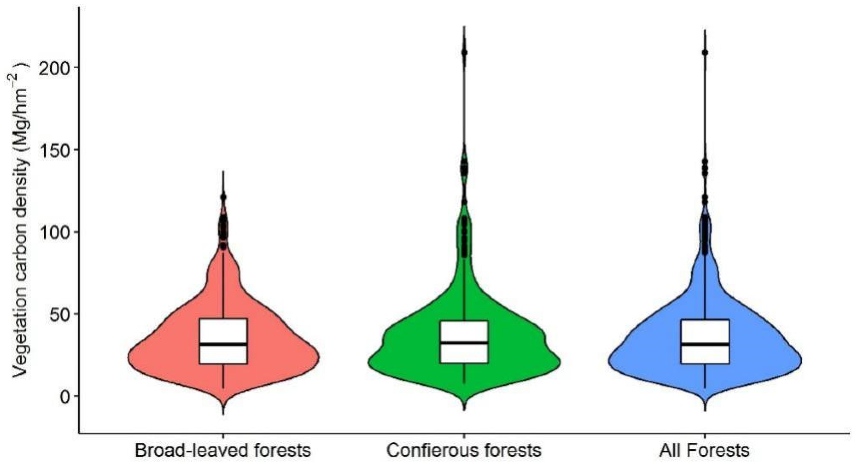
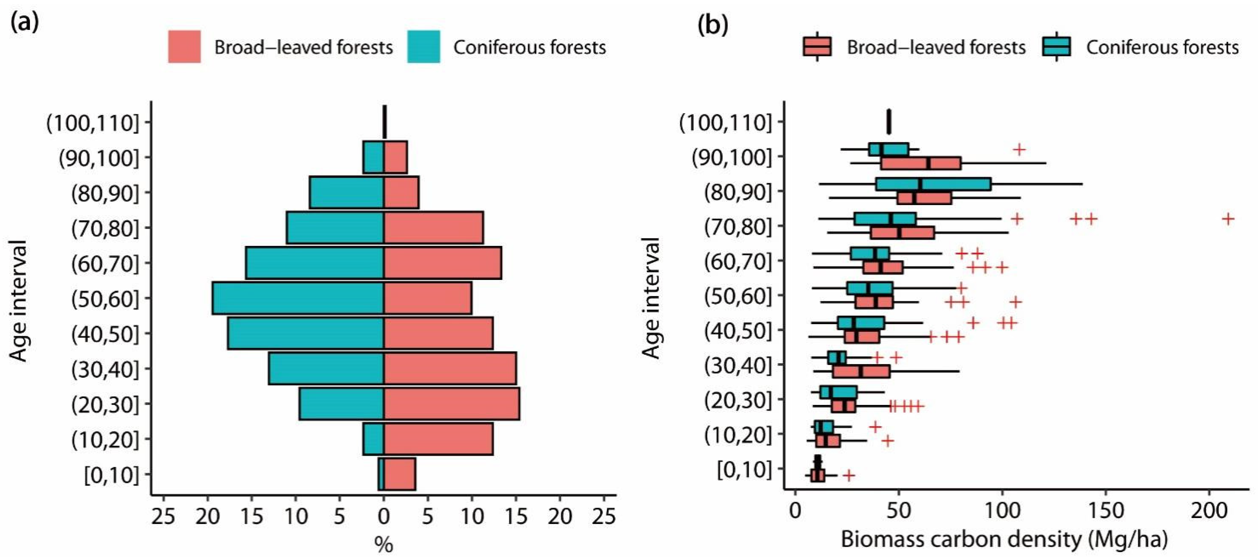
3.1. Biomass Carbon Density

The BCDs of all natural mountain forests in Shanxi varied from 4.79 to 209.16 Mg/ha, with a median value of 31.53 Mg/ha. There was no significant difference between the mean BCDs of coniferous and broad-leaved forests (p > 0.05), but the coefficient of variation of BCDs was larger for coniferous forests (72.93%) than broad-leaved forests (57.35%) (Figure 2). For all the natural forests, the average BCD of live trees was 30.06 Mg/ha, accounting for 82.4% of the total biomass carbon density (Table 2). The mean BCD of live trees also showed no significant difference between the broad-leaved and coniferous forests (p > 0.05). However, the mean BCD of undergrowth including shrubs and herbs was larger for the coniferous than broad-leaved forests.
Pinus tabulaeformis forests and Quercus liaotungensis forests were the dominant forest types for the coniferous and broad-leaved forests, respectively, accounting for 51.01% and 38.27% of the corresponding total area (Table 2, Figure S4). The mean BCDs of the arbor layer, undergrowth layer, and the total of them for Pinus tabulaeformis were significantly lower than those for Quercus liaotungensis forests (p< 0.01).
Mean BCDs of natural forests for different age groups were 25.93 Mg/ha (young), 48.29 Mg/ha (middle-aged), 68.35 Mg/ha (near matured), 81.44 Mg/ha (matured), and 74.67 Mg/ha (over-matured) (Figure S5). Across all five age groups except the middle-aged group, the mean BCDs of coniferous forests was lower than that of broad-leaved forests (p < 0.05) (Figure S5). Similarly, although the age structures of coniferous forest and broad-leaved forest were different, the mean BCD of the former was almost lower than that of the latter for all age intervals. The BCDs increased with forest ages for both the coniferous and broad-leaved forests, which were maximum near 85 yr and 95 yr, respectively (Figure 3). For the age structure and the relationship between BCDs and stand ages, Quercus liaotungensis forest is similar to the natural broad-leaved forest; Pinus tabulaeformis forest is similar to the natural coniferous forest (Figure S4).

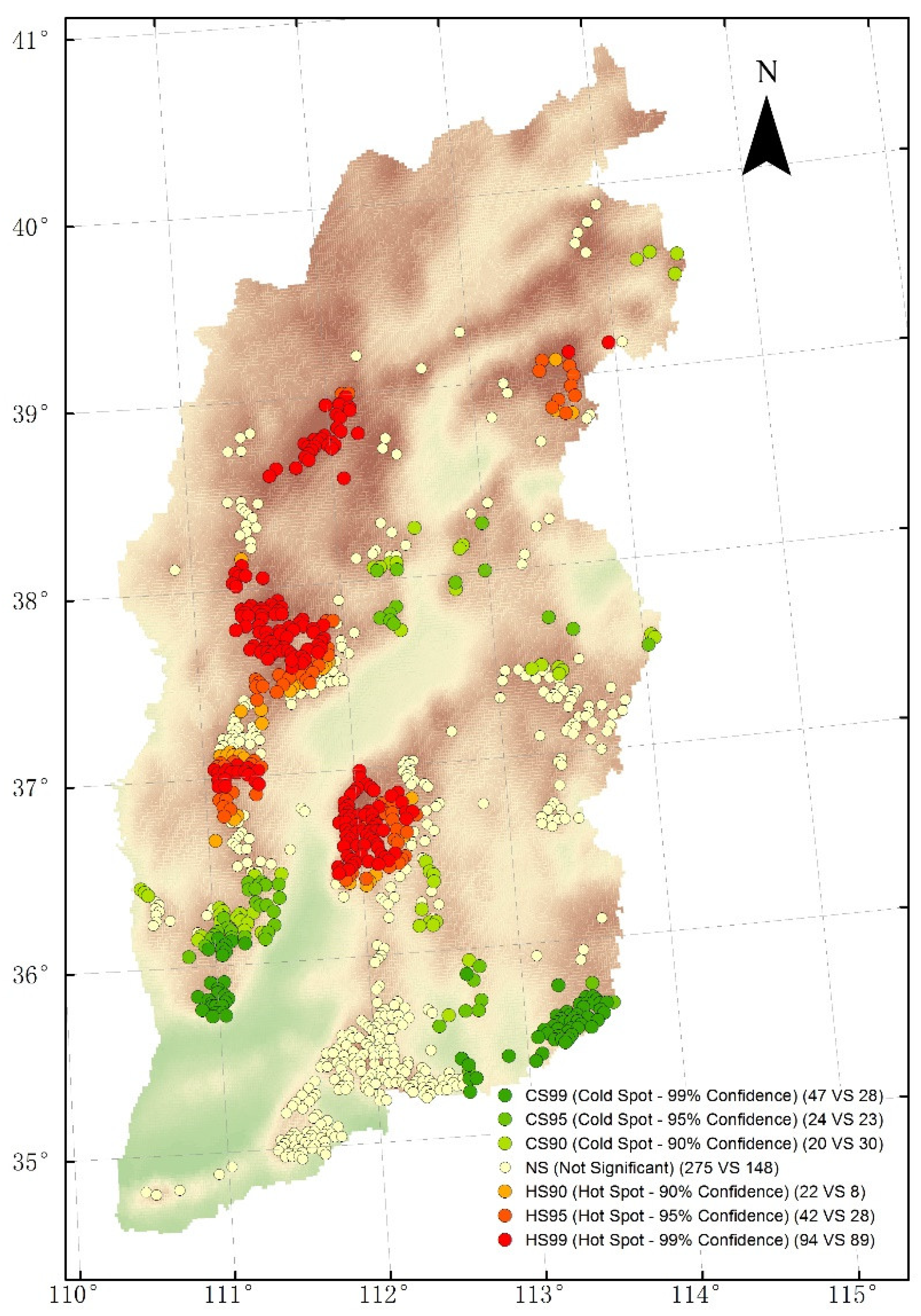
3.2. Spatial Hot Spots and Cold Spots Analyses for Biomass Carbon Densities

Anselin Local Moran’s I analysis showed that 283 hot spots and 170 cold spots were detected by Getis-ord G* for BCDs of natural mountain forests in our study area (Figure 4). The total number of spots with spatial autocorrelation accounted for 51.6% of all plots of the natural forests. The hot spots of biomass carbon density were distributed in the north of 36.5° N in Shanxi, mainly including Luya Mountain, Guandi Mountain, Wutai Mountain, Taiyue mountain, and some areas of the south-central part of the Lüliang Mountains. The cold-spots were found in the south of 36.5° N in Shanxi, mainly including the southernmost areas of the Lüliang Mountains and the southernmost areas of the Taihang Mountains. Besides, biomass carbon densities were randomly distributed in the entire areas of Zhongtiao mountain and the middle part of the Taihang Mountains.
Hot spots at the 1% significance level (HS99s), which have the highest average biomass carbon density of 47.86 Mg/ha, were distributed in the areas with an elevation of 1500–2000 m, the mean annual temperature of 8–10.8 °C, and the mean annual precipitation of 450–490 mm (Figure S6). Compared with the deciduous broad-leaved forests, HS99s for the coniferous forests were located in the areas with higher average latitude, higher average elevation, lower mean temperature, and lower mean precipitation (Figure S6). Overall, HS99s were mainly located in Luya Mountain, Guandi Mountain, and Taiyue Mountain from north to south (Figure 4). In Luya Mountain, the number of HS99s for coniferous forests (18) dominated by Picea wilsonii forests and Larix principis-rupprechtii forests was more than that for deciduous broad-leaved forests (11) dominated by Betula platyphylla forests and Quercus liaotungensis forests. In Guandi Mountain, the number of HS99s for coniferous forests (42) dominated by Pinus tabuliformis forests and coniferous mixed forests was more than that for deciduous broad-leaved forests (27) dominated by Quercus liaotungensis forests. In Taiyue Mountain, the number of HS99s for deciduous broad-leaved forests (39) mainly distributed in the west and dominated by Quercus liaotungensis forests and broad-leaved mixed forests was more than that for coniferous forests (27) mainly distributed in the east and dominated by Pinus tabuliformis forests. Generally, the number of HS99s for coniferous forests was higher than that for deciduous broad-leaved forests in the northern mountainous areas, but the contrary was true in the southern mountainous areas of Shanxi province.

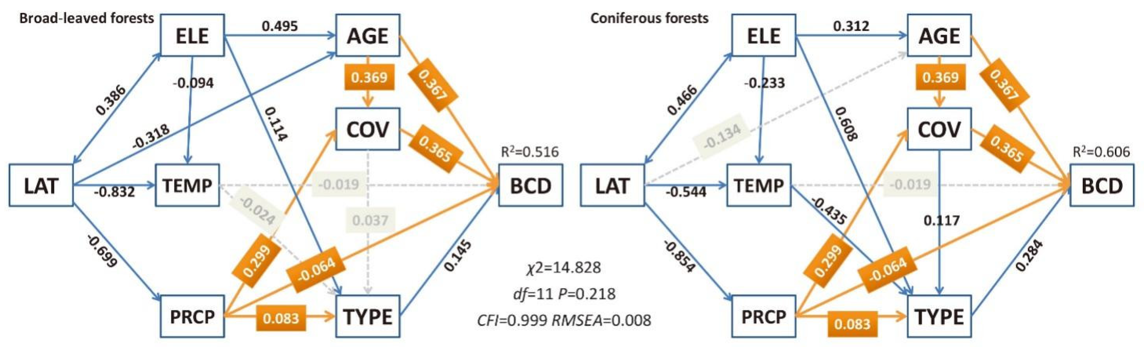
3.3. Influences of Various Factors on Biomass Carbon Density of Natural Mountain Forests

The multi-group SEM analysis revealed variation in path coefficients between natural coniferous and deciduous broad-leaved forests in the mountainous area (Figure 5). Except for the six paths from AGE to BCD and COV, PRCP to COV, BCD and TYPE, and AGE to COV, the remaining path coefficients were not equal between coniferous and deciduous broad-leaved forests. The seven factors included in our model could better explain the variation in BCD for coniferous forests (60.6%) than deciduous broad-leaved forests (51.6%) (Figure 5). AGE and COV showed a direct and positive association with BCD consistently for coniferous and deciduous broad-leaved forests (Figure 6). The effect of TYPE on BCD was stronger for the coniferous forests than the deciduous broad-leaved forests. ELE (LAT) had only indirect effects on BCD with the stronger total effect of ELE (LAT) for coniferous forests than deciduous broad-leaved forests. TEMP only had a negative indirect effect for coniferous forests and zero effect on BCD for deciduous broad-leaved forests. Due to the different effects of TYPE on BCD, PRCP had a slightly stronger total effect on BCD for the coniferous forests than deciduous broad-leaved forests, although it had equally direct effects on BCD for the two forest types. In short, the results of standardized total effects (Figure 6) indicated that, for the two forest types, stand factors (AGE, COV, and TYPE) and ELE were important driving factors of BCD, and climatic factors (TEMP and PRCP) had weaker effects on BCD relative to other factors. Compared with broad-leaved forests, stand factors (AGE, COV, and TYPE), geographical factors (LAT and ELE) and climatic factors (TEMP and PRCP) had stronger effects for the coniferous forests.

4. Discussion

4.1. Spatial Patterns of Biomass Carbon Density

The results of spatial hot spots and cold spots analyses showed that the areas in which the plots with high biomass carbon density distributed continuously in space were identified as hot spots areas (Figure 4). These hot spots were widely distributed in the mountainous areas with higher elevation (Figure S6), in most of which natural reserves were established, for instance, Luyashan National Natural Reserve in Luya Mountain, Pangquangou National Natural Reserve in Guandi Mountain, and Lingkongshan National Natural Reserve in Taiyue Mountain. In these reserves, the forests were less disturbed by human activities and would be relatively older. Meanwhile, the coniferous forests in hot spot areas consisted of Picea wilsonii forests, Larix principis-rupprechtii forests, coniferous mixed forests, and Pinus tabulaeformis forests, and deciduous broad-leaved forests consisted of Quercus liaotungensis forests, Betula platyphylla forests, and deciduous broad-leaved mixed forests. Compared with the total average biomass carbon density of natural forests, these forests had higher mean biomass carbon densities (Table 2). This promoted the formation of hot spots in these areas. Meanwhile, continuous distribution of the natural coniferous (deciduous broad-leaved) forests also helped to form hot spots areas in these areas (Figure 1b). In addition, the composition of tree species in hot spots areas was also relatively simple, and every tree species was widely distributed and concentrated in groups (Figure S1). This also reduced the inhomogeneity of spatial distribution of biomass carbon density in space due to the differences among forest types in these areas (Figure 5 and Figure 6), which was unfavorable for collection of information on the hot spots.
In contrast to the hot spots, the cold spots for biomass carbon density of natural mountain forests were mainly detected in or around the coal mining areas. Shanxi province, being abundant in coal resources, is one of the best important providers of coal in China [43]. For instance, cold spots at the 1% significance level (CS99s) in the southernmost tip of the Lüliang Mountains are located in Xiangning colliery, which is part of Hedong coalfield [44,45]. Another CS99s region detected in the south of Taihang Mountains lies to the east of Lingchuan colliery and in the Jincheng colliery, which belongs to Qinshui coalfield [44,45]. Higher impacts of long-term mining activities would lead to low forest biomass carbon densities and the formation of cold-spots in these areas.
The Zhongtiao Mountain, known as “Shanxi natural botanical garden” [46], is a key region for the woody flora of North China, in which many rare and endangered plants were distributed. In our study, the entire mountain was identified as an area of random distribution for the biomass carbon densities of natural mountain forests (Figure 4). The most likely explanation for this is that rich and varied plant species are randomly distributed in space (Figure 1b). On the other hand, it is well known that the mountain is one of the birthplaces of Chinese civilization, and that the emperors of Yao, Shun, Yu, and Tang had been here many times [46]. With the continuous expansion of agricultural production and the increasing population density around the mountain, human activities have had a more and more profound impact on natural forest vegetation in the course of history. Meanwhile, in ancient times the area was an important center for copper mining [47] and is today one of the operational bases of Zhongtiao Mountain Non-ferrous Metals Group Co., Ltd., one of China’s largest metal processing companies. Therefore, long-term mining and processing of mineral resources has also been producing a negative effect on natural forests in the mountains. Besides, the continuous development and utilization of tourism resources in the mountain could also be a reason for the random distribution of biomass carbon densities in Zhongtiao Mountain. In a word, frequent human disturbance is also be a decisive factor that cannot be ignored.

4.2. The Relationships between Stand Factors and Biomass Carbon Densities

The results of SEM analysis showed that AGE and COV were important predictors in modulating the BCD for mountainous coniferous and deciduous broad-leaved forests. Especially for the deciduous broad-leaved forests, effects of AGE and COV were stronger than that of the other factors (Figure 6). The findings were in agreement with Xu et al. [6] who found that canopy density and forest age were the dominant determinants of vegetation carbon density in subtropical forest ecosystems in Zhejiang Province, China. The strong positive effect of AGE on BCD, possibly because the stand age controls the duration of forest carbon accumulation [48] and biomass carbon density increases with stand development [49,50]. Owing to nutrient limitation, however, stomatal constraint and decline in photosynthesis during the stand development, mean that stand net primary productivity (NPP) declines along with the increase of tree age [51,52,53]. More importantly, in mature forests, tree size and local competition are important predictors of mortality risk, and tree mortality increases over time in the stand development processes [54]. Increasing mortality in old forests not only slows down the rate of biomass accumulation but also increases the biomass losses in the vegetation due to the increases of litterfall from the trees and decomposition losses. The factors mentioned above tend to move the biomass/carbon storage in the old forests toward a steady state [55]. In our study, we found that equilibrium points were about 95 yr and 85 yr for mountainous broad-leaved and coniferous forests in our study area, respectively (Figure 3b).
Meanwhile, TYPE was another stand factor in modulating the BCD for the mountainous forests. The effect of TYPE on BCD was greater for the coniferous forests than the deciduous broad-leaved forests (Figure 6). The result could be due to the differences of averaged BCDs of different forest types between the coniferous and broad-leaved forests. The further result showed that the difference of mean BCDs of different forest types for the coniferous forests was significantly larger than that for the broad-leaved forests (Table 2) (t = 0.973, p = 0.058).

4.3. The Effects of Geographical Factors on Biomass Carbon Density

Compared with other geographical factors (longitude, slope aspect, and slope position), the introduction of ELE and LAT into our model could be mainly determined by the special geographical environment conditions of mountainous forests in our study. Deciduous broad-leaved forests and coniferous forests ranged from 520 m to 2309 m and from 483 m to 2560 m in elevation, respectively. Elevation gradient is associated with changes in temperature and precipitation, and forest type [20]. By regulating moisture and soil water availability [19], elevation can affect forest canopy, stem density, and stand basal area, and therefore affect aboveground biomass [5,6]. Therefore, the larger elevation gradient of the natural forests could probably lead to the significant effects of ELE on BCD in the mountainous terrain of the Shanxi plateau. Similarly, based on the SEM, Xu et al. [6] also reported that altitude was the most important abiotic driving factor of vegetation carbon stocks in Zhejiang Province, China. Furthermore, a positive effect of ELE on BCD was detected for natural coniferous and deciduous broad-leaved forests in our study (Figure 6). Similar results were also reported by Liu et al. [18], who found a positive linear relationship between vegetation carbon stock and altitude across three forests (Larix principis-rupprechtii (LP) forest, Picea meyerii (PM) forest, and Pinus tabulaeformis (PT) forest) on Loess Plateau in an altitudinal range of 1200–2700 m. In addition, a similar relationship between biomass carbon density and elevation was reported by Sumeet Gairola et al. [17] in moist temperate forests of the Garhwal Himalaya.
LAT also had a significant effect on BCD in our study due to the fact that the distribution of natural forests also had a larger latitude span. Natural deciduous broad-leaved forests and coniferous forests ranged from 34.79° to 39.89° and from 34.97° to 39.75° in latitude, respectively. The large latitude span would lead to great changes in environmental conditions along latitude gradients from the north to the south, including the light, heat, and moisture, and would affect plant growth and therefore influence the biomass carbon accumulation in the natural forests from the north to the south. It is noteworthy that in the areas of natural forests in our study, the higher the latitude, the higher was the elevation (r = 0.708, p < 0.001, n = 878). So, the positive relationship of LAT with ELE enhanced the total effects of LAT and ELE to BCD (Figure 6). In previous studies [56], we had found that there was a significant positive correlation between latitude and altitude in the Loess Plateau Region (r = 0.211, p < 0.003, n = 196), in which our entire study region was included, and a significant negative correlation between them in Tibet Plateau (r = −0.544, p < 0.001, n = 66). Therefore, we have reason to believe that the positive relationship of LAT with ELE should enhance the total effects of LAT and ELE on BCD in the whole Loess Plateau Region, while the negative relationship between them should weaken the total effects of LAT and ELE on BCD in Tibet Plateau.

4.4. The Effects of Climatic Factors on Biomass Carbon Density

The total effects of climatic factors (TEMP and PRCP) were lower than those of geographical factors (ELE and LAT) and stand factors (AGE, COV, and TYPE) in temperate mountainous forests in Shanxi. According to the SEM, we found a negative effect of TEMP on BCD for the natural coniferous forests, indicating that the lower the temperature, the higher the BCD of the forest. It could be the result of natural selection of the coniferous tree species for the site conditions and the spatial distribution of these tree species in our study. For example, the Picea and Larix principis-rupprechtii forests with the higher mean biomass carbon densities were generally distributed in the regions with lower temperatures, but Platycladus orientalis forests with the lowest mean biomass carbon density were generally distributed in warmer areas (Table 1). A similar result was also found by Fehse et al. [57], who demonstrated that forests under favorable site conditions at high altitudes with low temperatures were not inferior in biomass accumulation and productivity compared to forests at low altitude with high temperature. Meanwhile, the smaller leaf surface area of coniferous trees which reduces water and heat loss is beneficial to cold resistance. The lower temperature for mountainous coniferous forests in our study would not greatly limit the photosynthetic carbon sequestration rate of these coniferous trees but the amount of carbon released by respiration might be substantially reduced because respiration generally requires a higher temperature than photosynthesis. Consequently, lower temperatures for coniferous forests probably increased the biomass carbon accumulation. However, another possible explanation is that precipitation and, to some extent, temperature are not what trees are actually responding to. They may be responding to water availability. If the temperature decreases, then for a given level of precipitation, water becomes more available because less evaporates (or transpiration losses are reduced). In fact, for the temperate deciduous broad-leaved forests, which were the zonal vegetation in our study area, TEMP had no significant effect on BCD. Similarly, Liu et al. [26] also found that a nonlinear relationship exists between the above-ground biomass carbon density and mean annual temperature in the temperate mountain system for mature forests on the global scale.

4.5. Integrative Framework of Biomass Carbon Density for the Mountainous Forests

Numerous studies on the factors influencing forest carbon storage in mountainous areas focused only on the effects of elevation on forest carbon storage [11,17,18,58,59]. A very small number of studies focused on the interaction between different influencing factors, and the indirect effects of these factors on forest carbon storage. In our study, an integrative framework of biomass carbon density for the mountainous forests was proposed, which combined three kinds of driving factors, including stand (AGE, COV, and TYPE), climatic (TEMP and PRCP), and geographical factors (ELE and LAT), and then the direct and indirect effects of these factors on biomass carbon density were derived from it. For example, we found that geographical factors had affected biomass carbon density indirectly in our study (Figure S2). In detail, ELE had affected BCD through the direct effects of ELE on TYPE, AGE, and TEMP (Figure S2). Meanwhile, we also found a positive relationship between ELE and AGE (Figure 5). This was probably because the forests at higher elevations had usually experienced little disturbance, and could grow steadily and presented larger average stand age. Moreover, ELE had effects on the distribution of the coniferous forest types for the coniferous forests. Noticeably, for coniferous forests, the Picea and Larix principis-rupprechtii forests were generally distributed at a higher elevation than Pinus tabuliformis and Platycladus orientalis forests across the entire region (Table 1), and the BCDs for the former two were generally greater than for the latter two (Table 2). In short, the indirect effects were helpful for us to understand why elevation was an important driving factor of biomass carbon density for mountain forests and how geographical factors affect biomass carbon density in our study.
Meanwhile, multi-group SEM as an integrative approach also was used to compare the groups in our study. It could be revealed whether the effects of these factors were consistent between the coniferous forests and broad-leaved forests. For instance, the effect of AGE (COV) on BCD for the coniferous forests was equal to that for deciduous broad-leaved forests, but the effects of climatic and geographical factors varied greatly between them. For the deciduous broad-leaved forests, the positive connection between ELE and AGE was the main reason for the positive effects of ELE on BCD. In contrast, for the coniferous forests, ELE had effects on TEMP and TYPE besides the positive effect on AGE (Figure 5). Therefore, the total effect of ELE on BCD was different as between the deciduous broad-leaved and coniferous forests (Figure 6). Furthermore, if we did not use the multi-group SEM, the model we proposed in our study, the qualitative structure of which was correct would be incorrectly rejected because the coniferous forests and deciduous broad-leaved forests differ in the numerical strength of these causal relationships.
To verify our integrative framework, we also used stepwise regression analysis to identify all factors which had significant effects on BCD. The results showed that the main influencing factors for natural broad-leaved forests were AGE > COV > ELE > TYPE (BCD = 0.388 × AGE + 0.316 × COV + 0.190 × ELE + 0.147 × TYPE, p < 0.0001, R2 = 0.531), while those for natural coniferous forests were COV > AGE > ELE > TYPE (BCD = 0.383 × COV + 0.345 × AGE + 0.303 × ELE + 0.270 × TYPE, p < 0.0001, R2 = 0.668). Obviously, the four factors of AGE, COV, ELE, and TYPE were also identified as the most important explanatory variables for the BCD of the two forest types. Furthermore, for the relative contribution of the four factors to BCD of natural broad-leaved forests, the result of stepwise regression analysis was identical to that of our SEMs (Figure 6). For coniferous forests, the result of stepwise regression analysis was almost consistent with that of SEMs. This proved that our SEMs were reasonable and correct.

5. Conclusions

In our study, we found that there was no significant difference between the mean biomass carbon density for the natural coniferous forests and that for the natural deciduous broad-leaved forests in Shanxi, China, while the coefficient of variation of biomass carbon densities was larger in the coniferous forest than in deciduous broad-leaved forests. There was no significant difference between the mean biomass carbon densities of the natural coniferous and broad-leaved forests. The spatial patterns of biomass carbon densities for the natural forests were associated with the geographical conditions, forest type distribution, human interference density, and the implementation of natural forest resources protection measures in Shanxi Province. Compared with the deciduous broad-leaved forests, hot-spots at the 1% significance level (HS99s) for the coniferous forests, which have the highest average biomass carbon density of 47.86 Mg/ha, were distributed in the areas with higher average latitude, higher average elevation, lower mean temperature, or lower mean precipitation.
Multi-groups structural equation modeling that combined stand, geographical, and climatic factors was used to compare the effects of these factors on biomass carbon densities between the natural coniferous forests and the natural deciduous broad-leaved forests in mountainous areas. These factors, including latitude (LAT), elevation (ELE), mean annual temperature (TEMP), mean annual precipitation (PRCP), stand age (AGE), coverage (COV), and forest type (TYPE) could explain 60.6% of the variation in biomass carbon density for coniferous forests and 51.6% for deciduous broad-leaved forests. Stand factors (AGE, COV, and TYPE) and ELE were important driving factors of BCD, and climatic factors (TEMP and PRCP) had weaker effects on BCD relative to other factors. Compared with broad-leaved forests, stand factors (AGE, COV, and TYPE), geographical factors (LAT and ELE), and climatic factors (TEMP and PRCP) had stronger effects for the coniferous forests. Among all driving factors, AGE had the strongest total effect for the two forest types. This study enhances the understanding of variation in the biomass carbon density in natural coniferous forests and deciduous broad-leaved forests in the mountainous region and should be beneficial for more effective implementation of afforestation and forest protection programs to enhance biomass carbon sequestration and mitigate global climate change.

Supplementary Materials

The following supporting information can be downloaded at: https://www.mdpi.com/article/10.3390/f13071114/s1, Figure S1: Maps showing the distribution of the sample plots for the investigation of biomass carbon density for natural broad-leaved and coniferous forests in Shanxi, China. Figure S2: The exploratory structure equation models showing the geographical, climatic and stand factors that have direct and indirect effects on BCD (biomass carbon density) of natural broad-leaved and coniferous forests in Shanxi, China. Figure S3: The good-fitting structure equation models showing the factors that have direct and indirect effects on biomass carbon density of broad-leaved (left) and coniferous (right) forests in Shanxi, China. Figure S4: Average biomass carbon density of different age intervals of natural broad-leaved and coniferous forests in Shanxi, China. Figure S5: Average biomass carbon density of different age groups (left) and different age intervals (right) of natural broad-leaved and coniferous forests in Shanxi, China. Figure S6: The plot showing the changes of different factors with the hot spots groups at different significant levels (right) of natural broad-leaved and coniferous forests in Shanxi, China. Tables S1: Direct, indirect, and total effects of stand age (AGE), stand coverage (COV), forest type (TYPE), elevation (ELE), latitude (LAT), mean annual temperature (TEMP) and precipitation (PRCP) on biomass carbon density for natural coniferous forests. Table S2: Same as Table S1 but for natural broad-leaved forests.

Author Contributions

Conceived and designed the study: L.S. and X.F. Analyzed the data: L.S., Q.W. and X.F. Wrote the paper: L.S., Q.W. and X.F. All authors have read and agreed to the published version of the manuscript.

Funding

This study was funded by the Natural Science Foundation for Young Scientists of Shanxi Province (grant No. 20210302124493 & 201901D211420), and Scientific and Technological Innovation Programs of Higher Education Institutions in Shanxi Province (STIP 2019L0807).

Data Availability Statement

Not applicable.

Acknowledgments

We acknowledge the Carbon Sequestration Monitoring Center of Forestry Investigation and Planning Institute in Shanxi for providing us with national forest inventory data as well as useful advice for their manipulation. This study was funded by the Natural Science Foundation for Young Scientists of Shanxi Province (grant No.20210302124493 & 201901D211420), and Scientific and Technological Innovation Programs of Higher Education Institutions in Shanxi Province (STIP 2019L0807).

Conflicts of Interest

The authors declare no conflict of interest. The funders had no role in the design of the study; in the collection, analyses, or interpretation of data; in the writing of the manuscript, or in the decision to publish the results.

References

  1. IPCC. IPCC Climate Change 2014: Synthesis Report; Contribution of Working Groups I, II and III to the Fifth Assessment Report of the Intergovernmental Panel on Climate Change; Core Writing Team, Pachauri, R.K., Meyer, L.A., Eds.; IPCC: Geneva, Switzerland, 2014.
  2. FAO. FAO Global Forest Resources Assessment. 2020. Available online: https://www.fao.org/forest-resources-assessment/en/ (accessed on 15 July 2022).
  3. Chave, J.; Condit, R.; Lao, S.; Caspersen, J.P.; Foster, R.B.; Hubbell, S.P. Spatial and Temporal Variation of Biomass in a Tropical Forest: Results from a Large Census Plot in Panama. J. Ecol. 2003, 13, 240–252. [Google Scholar] [CrossRef]
  4. Slik, J.W.F.; Aiba, S.-I.; Brearley, F.Q.; Cannon, C.H.; Forshed, O.; Kitayama, K.; Nagamasu, H.; Nilus, R.; Payne, J.; Paoli, G.; et al. Environmental Correlates of Tree Biomass, Basal Area, Wood Specific Gravity and Stem Density Gradients in Borneo’s Tropical Forests. Glob. Ecol. Biogeogr. 2010, 19, 50–60. [Google Scholar] [CrossRef]
  5. Xu, M.; Ji, H.; Zhuang, S. Carbon Stock of Moso Bamboo (Phyllostachys Pubescens) Forests along a Latitude Gradient in the Subtropical Region of China. PLoS ONE 2018, 13, e0193024. [Google Scholar] [CrossRef] [Green Version]
  6. Xu, L.; Shi, Y.; Fang, H.; Zhou, G.; Xu, X.; Zhou, Y.; Tao, J.; Ji, B.; Xu, J.; Li, C. Vegetation Carbon Stocks Driven by Canopy Density and Forest Age in Subtropical Forest Ecosystems. Sci. Total. Environ. 2018, 631–632, 619–626. [Google Scholar] [CrossRef] [PubMed]
  7. Wei, Y.; Li, M.; Chen, H.; Lewis, B.J.; Yu, D.; Zhou, L.; Zhou, W.; Fang, X.; Zhao, W.; Dai, L. Variation in Carbon Storage and Its Distribution by Stand Age and Forest Type in Boreal and Temperate Forests in Northeastern China. PLoS ONE 2013, 8, e72201. [Google Scholar] [CrossRef] [PubMed] [Green Version]
  8. Price, M.F.; Butt, N.; International Union of Forestry Research Organizations (Eds.) Forests in Sustainable Mountain Development: A State of Knowledge Report for 2000; IUFRO Research Series; CABI Pub.: Wallingford, UK; International Union of Forestry Research Organizations: New York, NY, USA, 2000; ISBN 978-085-199-446-8. [Google Scholar]
  9. Li, S.; Hu, S.; Tang, X. Dynamic Change of Forest Carbon Stocks; Science Press: Beijing, China, 2013; ISBN 978-7-03-037127-0. [Google Scholar]
  10. Investigation and Planning Institute of the Ministry of forestry of China. The Mountain Forests in China; China Forestry Publishing House: Beijing, China, 1981.
  11. Chang, R.; Wang, G.; Fei, R.; Yang, Y.; Luo, J.; Fan, J. Altitudinal Change in Distribution of Soil Carbon and Nitrogen in Tibetan Montane Forests. Soil Sci. Soc. Am. J. 2015, 79, 1455–1469. [Google Scholar] [CrossRef]
  12. Zald, H.S.J.; Spies, T.A.; Seidl, R.; Pabst, R.J.; Olsen, K.A.; Steel, E.A. Complex Mountain Terrain and Disturbance History Drive Variation in Forest Aboveground Live Carbon Density in the Western Oregon Cascades, USA. For. Ecol. Manag. 2016, 366, 193–207. [Google Scholar] [CrossRef] [Green Version]
  13. Fu, W.; Fu, Z.; Ge, H.; Ji, B.; Jiang, P.; Li, Y.; Wu, J.; Zhao, K. Spatial Variation of Biomass Carbon Density in a Subtropical Region of Southeastern China. Forests 2015, 6, 1966–1981. [Google Scholar] [CrossRef] [Green Version]
  14. Lin, Z.; Chao, L.; Wu, C.; Hong, W.; Hong, T.; Hu, X. Spatial Analysis of Carbon Storage Density of Mid-Subtropical Forests Using Geostatistics: A Case Study in Jiangle County, Southeast China. Acta Geochim. 2017, 37, 90–101. [Google Scholar] [CrossRef]
  15. Ren, H.; Chen, H.; Li, L.; Li, P.; Hou, C.; Wan, H.; Zhang, Q.; Zhang, P. Spatial and Temporal Patterns of Carbon Storage from 1992 to 2002 in Forest Ecosystems in Guangdong, Southern China. Plant Soil 2013, 363, 123–138. [Google Scholar] [CrossRef]
  16. Dai, W.; Fu, W.; Jiang, P.; Zhao, K.; Li, Y.; Tao, J. Spatial Pattern of Carbon Stocks in Forest Ecosystems of a Typical Subtropical Region of Southeastern China. For. Ecol. Manag. 2018, 409, 288–297. [Google Scholar] [CrossRef]
  17. Gairola, S.; Sharma, C.M.; Ghildiyal, S.K.; Suyal, S. Live Tree Biomass and Carbon Variation along an Altitudinal Gradient in Moist Temperate Valley Slopes of the Garhwal Himalaya (India). Curr. Sci. India 2011, 100, 1862–1870. [Google Scholar]
  18. Liu, N.; Nan, H. Carbon Stocks of Three Secondary Coniferous Forests along an Altitudinal Gradient on Loess Plateau in Inland China. PLoS ONE 2018, 13, e0196927. [Google Scholar] [CrossRef] [PubMed] [Green Version]
  19. Fisk, M.C.; Schmidt, S.K.; Seastedt, T.R. Topographic Patterns of Above- and Belowground Production and Nitrogen Cycling in Alpine Tundra. Ecology 1998, 79, 2253–2266. [Google Scholar] [CrossRef]
  20. Sanaei, A.; Chahouki, M.A.Z.; Ali, A.; Jafari, M.; Azarnivand, H. Abiotic and Biotic Drivers of Aboveground Biomass in Semi-Steppe Rangelands. Sci. Total Environ. 2018, 615, 895–905. [Google Scholar] [CrossRef]
  21. Wen, D.; He, N. Forest Carbon Storage along the North-South Transect of Eastern China: Spatial Patterns, Allocation, and Influencing Factors. Ecol. Indic. 2016, 61, 960–967. [Google Scholar] [CrossRef]
  22. Fan, Y.Q.; Zhou, G.M.; Shi, Y.J.; Dong, D.J.; Zhou, Y.F. Relationship of Slope Aspect and Position on Biomass and Carbon Storage in a Phyllostachys Edulis Stand. J. Zhejiang A F Univ. 2012, 29, 321–327. [Google Scholar]
  23. Durán, S.M.; Sánchez-Azofeifa, G.A.; Rios, R.S.; Gianoli, E. The Relative Importance of Climate, Stand Variables and Liana Abundance for Carbon Storage in Tropical Forests: Climate, Stand Variables and Lianas Control Forest Carbon. Glob. Ecol. Biogeogr. 2015, 24, 939–949. [Google Scholar] [CrossRef]
  24. Stegen, J.C.; Swenson, N.G.; Enquist, B.J.; White, E.P.; Phillips, O.L.; Jørgensen, P.M.; Weiser, M.D.; Monteagudo Mendoza, A.; Núñez Vargas, P. Variation in Above-Ground Forest Biomass across Broad Climatic Gradients. Glob. Ecol. Biogeogr. 2011, 20, 744–754. [Google Scholar] [CrossRef]
  25. Xu, B.; Guo, Z.D.; Piao, S.L.; Fang, J.Y. Biomass Carbon Stocks in China’s Forests between 2000 and 2050: A Prediction Based on Forest Biomass-Age Relationships. Sci. China Life Sci. 2010, 53, 776–783. [Google Scholar] [CrossRef]
  26. Liu, Y.; Yu, G.; Wang, Q.; Zhang, Y. How Temperature, Precipitation and Stand Age Control the Biomass Carbon Density of Global Mature Forests. Glob. Ecol. Biogeogr. 2014, 23, 323–333. [Google Scholar] [CrossRef]
  27. Shipley, B. Cause and Correlation in Biology: A User’s Guide to Path Analysis, Structural Equations and Causal Inference with R, 2nd ed.; Cambridge University Press: Cambridge, UK, 2016; ISBN 978-110-744-259-7. [Google Scholar]
  28. Delgado-Baquerizo, M.; Grinyer, J.; Reich, P.B.; Singh, B.K. Relative Importance of Soil Properties and Microbial Community for Soil Functionality: Insights from a Microbial Swap Experiment. Funct. Ecol. 2016, 30, 1862–1873. [Google Scholar] [CrossRef]
  29. Grace, J.B.; Anderson, T.M.; Olff, H.; Scheiner, S.M. On the Specification of Structural Equation Models for Ecological Systems. Ecol. Monogr. 2010, 80, 67–87. [Google Scholar] [CrossRef] [Green Version]
  30. Ali, A.; Yan, E.-R.; Chen, H.Y.H.; Chang, S.X.; Zhao, Y.T.; Yang, X.D.; Xu, M.S. Stand Structural Diversity Rather than Species Diversity Enhances Aboveground Carbon Storage in Secondary Subtropical Forests in Eastern China. Biogeosciences 2016, 13, 4627–4635. [Google Scholar] [CrossRef] [Green Version]
  31. Jonsson, M.; Wardle, D.A. Structural Equation Modelling Reveals Plant-Community Drivers of Carbon Storage in Boreal Forest Ecosystems. Biol. Lett. 2010, 6, 116–119. [Google Scholar] [CrossRef] [Green Version]
  32. Wang, Y.; Wang, Q.; Wang, M. Similar Carbon Density of Natural and Planted Forests in the Lüliang Mountains, China. Ann. For. Sci. 2018, 75, 87. [Google Scholar] [CrossRef] [Green Version]
  33. Wang, N. Study on Distribution Patterns of Carbon Density and Carbon Stock in the Forest Ecosystem of Shanxi; Beijing Forestry University: Beijing, China, 2014. (In Chinese) [Google Scholar]
  34. Ma, Z. Vegetation of Shanxi Province; China Science and Technology Press: Beijing, China, 2001; ISBN 978-750-463-108-4. (In Chinese) [Google Scholar]
  35. Fan, X.; Wang, M. Change Trends of Air Temperature and Precipitation over Shanxi Province, China. Theor. Appl. Climatol. 2011, 103, 519–531. [Google Scholar] [CrossRef]
  36. Xiao, X. National Forest Inventory of China; China Forestry Publishing House: Beijing, China, 2005. (In Chinese) [Google Scholar]
  37. Sun, L.; Wang, M.; Fan, X. Spatial Pattern and Driving Factors of Biomass Carbon Density for Natural and Planted Coniferous Forests in Mountainous Terrain, Eastern Loess Plateau of China. For. Ecosyst. 2020, 7, 9. [Google Scholar] [CrossRef] [Green Version]
  38. Lamsal, S.; Cobb, R.C.; Hall Cushman, J.; Meng, Q.; Rizzo, D.M.; Meentemeyer, R.K. Spatial Estimation of the Density and Carbon Content of Host Populations for Phytophthora Ramorum in California and Oregon. For. Ecol. Manag. 2011, 262, 989–998. [Google Scholar] [CrossRef]
  39. Plouffe, C.C.F.; Robertson, C.; Chandrapala, L. Comparing Interpolation Techniques for Monthly Rainfall Mapping Using Multiple Evaluation Criteria and Auxiliary Data Sources: A Case Study of Sri Lanka. Environ. Model. Softw. 2015, 67, 57–71. [Google Scholar] [CrossRef]
  40. Eldeiry, A.A.; Garcia, L.A. Comparison of Ordinary Kriging, Regression Kriging, and Cokriging Techniques to Estimate Soil Salinity Using LANDSAT Images. J. Irrig. Drain. Eng. 2010, 136, 355–364. [Google Scholar] [CrossRef]
  41. Manepalli, U.R.R.; Bham, G.H.; Kandada, S. Evaluation of Hot-Spots Identification Using Kernel Density Estimation and Getis-Ord on I-630. In Proceedings of the 3rd International Conference on Road Safety and Simulation, Indianapolis, IN, USA, 14–16 September 2011; Volume 9, pp. 14–16. [Google Scholar]
  42. Rosseel, Y. Lavaan: An R Package for Structural Equation Modeling. J. Stat. Soft. 2012, 48, 1–36. [Google Scholar] [CrossRef] [Green Version]
  43. Shanxi Geological Exploration Bureau. Mineral Exploration Results; Shanxi Geological Exploration Bureau: Taiyuan, China, 2018; Available online: http://www.sxdkj.com/ztzl/dzcj/2018-12-21/10221.html (accessed on 15 July 2022).
  44. Shi, J.R. Overview of geological and mineral resources in Shanxi Province. Land Resour. North China 2017, 4, 76–78. (In Chinese) [Google Scholar]
  45. Shanxi Fenwei Energy Development Consulting Co., Ltd. Shanxi Coal Resources Map. 2007. Available online: www.sxcoal.com (accessed on 15 July 2022).
  46. Zhang, F.; Wu, Y. Illuistration Handbook of Plants in Zhongtiao Mountains; China Forestry Publishing House: Beijing, China, 2015; ISBN 978-750-387-936-4. [Google Scholar]
  47. Chen, W.M.; Zhang, C.X.; Lu, J.R.; Dang, Z.F.; Li, S.P.; Cai, W.B.; Ning, Y.; Cao, Y.J. Polygenetic Mineralization of the Early Proterozoic Tongkuangyu Metaporphyry Copper Deposit in the Zhongtiao Mountains of China. Geotecton. Metallog. 1996, Z1, 110–111. [Google Scholar]
  48. Pregitzer, K.S.; Euskirchen, E.S. Carbon Cycling and Storage in World Forests: Biome Patterns Related to Forest Age. Glob. Change Biol. 2004, 10, 2052–2077. [Google Scholar] [CrossRef]
  49. Cheng, X.; Han, H.; Kang, F.; Song, Y.; Liu, K. Variation in Biomass and Carbon Storage by Stand Age in Pine (Pinus tabulaeformis) Planted Ecosystem in Mt. Taiyue, Shanxi, China. J. Plant Interact. 2014, 9, 521–528. [Google Scholar] [CrossRef]
  50. Fonseca, W.; Rey Benayas, J.M.; Alice, F.E. Carbon Accumulation in the Biomass and Soil of Different Aged Secondary Forests in the Humid Tropics of Costa Rica. For. Ecol. Manag. 2011, 262, 1400–1408. [Google Scholar] [CrossRef]
  51. Gower, S.T. Patterns and Mechanisms of the Forest Carbon Cycle. Ann. Rev. Env. Resour. 2003, 28, 169–204. [Google Scholar] [CrossRef]
  52. Mcdowell, G.R.; Harireche, O. Discrete Element Modelling of Yielding and Normal Compression of Sand. Géotechnique 2002, 52, 299–304. [Google Scholar] [CrossRef]
  53. Tang, J.; Luyssaert, S.; Richardson, A.D.; Kutsch, W.; Janssens, I.A. Steeper Declines in Forest Photosynthesis than Respiration Explain Age-Driven Decreases in Forest Growth. Proc. Natl. Acad. Sci. USA 2014, 111, 8856–8860. [Google Scholar] [CrossRef] [Green Version]
  54. Thorpe, H.C.; Daniels, L.D. Long-Term Trends in Tree Mortality Rates in the Alberta Foothills Are Driven by Stand Development. Can. J. For. Res. 2012, 42, 1687–1696. [Google Scholar] [CrossRef]
  55. Goulden, M.L.; Mcmillan, A.M.S.; Winston, G.C.; Rocha, A.V.; Manies, K.L.; Harden, J.W.; Bond-Lamberty, B.P. Patterns of NPP, GPP, Respiration, and NEP during Boreal Forest Succession: Carbon Dynamics during Boreal Succession. Glob. Change Biol. 2011, 17, 855–871. [Google Scholar] [CrossRef] [Green Version]
  56. Wang, Q.; Fan, X.; Wang, M. Recent Warming Amplification over High Elevation Regions across the Globe. Clim. Dynam. 2014, 43, 87–101. [Google Scholar] [CrossRef] [Green Version]
  57. Fehse, J.; Hofstede, R.; Aguirre, N.; Paladines, C.; Kooijman, A.; Sevink, J. High Altitude Tropical Secondary Forests: A Competitive Carbon Sink? For. Ecol. Manag. 2002, 163, 9–25. [Google Scholar] [CrossRef]
  58. Seedre, M.; Kopáček, J.; Janda, P.; Bače, R.; Svoboda, M. Carbon Pools in a Montane Old-Growth Norway Spruce Ecosystem in Bohemian Forest: Effects of Stand Age and Elevation. For. Ecol. Manag. 2015, 346, 106–113. [Google Scholar] [CrossRef]
  59. Zhu, B.A.; Wang, X.P.; Fang, J.Y.; Piao, S.L.; Shen, H.H.; Zhao, S.Q.; Peng, C.H. Altitudinal Changes in Carbon Storage of Temperate Forests on Mt Changbai, Northeast China. J. Plant Res. 2010, 123, 439–452. [Google Scholar] [CrossRef] [PubMed]
Figure 1. Maps showing the general topography in Shanxi Province (a) and the distribution of the sample plots for the investigation of biomass carbon density of natural broad-leaved and coniferous forests in the region (b). The number in parentheses denotes the number of the sample plots.
Forests 13 01114 g001
Figure 2. The kernel density estimation of natural broad-leaved and coniferous forests biomass carbon density in Shanxi, China.
Forests 13 01114 g002
Figure 3. Forest age structure (a) and average biomass carbon density (b) of different age intervals of natural broad-leaved and coniferous forests in Shanxi, China.
Forests 13 01114 g003
Figure 4. Map showing the spatial cold and hot spots of biomass carbon density in Shanxi, China. The number in parentheses is the number of sample plots.
Forests 13 01114 g004
Figure 5. Multi−group structural equation model for natural broad−leaved and coniferous forests. The factors influencing the biomass carbon density (BCD) of natural broad-leaved and coniferous forests include stand age (AGE), stand coverage (COV), forest type (TYPE), elevation (ELE), latitude (LAT), annual mean temperature (TEMP), and annual mean precipitation (PRCP). Solid arrows indicate significant paths (p < 0.05), while dashed arrows are non-significant paths. The numbers along the arrows are standardized regression weights indicating the effect size. R2 denotes the proportion of variation explained. Orange arrows represent equal effects between broad-leaved and coniferous forests; while blue arrows represent unequal effects between them.
Forests 13 01114 g005
Figure 6. Direct, indirect and total effects of stand age (AGE), stand coverage (COV), forest type (TYPE), elevation (ELE), latitude (LAT), mean annual temperature (TEMP) and precipitation (PRCP) on biomass carbon density for natural broad-leaved and coniferous forests. The detailed process of calculating direct and indirect effects of all factors on biomass carbon density shows in Tables S1 and S2 of Supplementary Materials.
Forests 13 01114 g006
Table 1. Descriptive statistics of elevation (ELE), latitude (LAT), annual mean temperature (TEMP) and annual precipitation (PRCP), stand age (AGE), stand coverage (COV) for natural broad-leaved and coniferous forests in Shanxi, China.
Forest TypeELE
(km)
LAT
(°)
TEMP
(°C)
PRCP
(mm)
AGE
(yr)
COV
(%)
Broad-leaved
forests
Quercus liaotungensis1522.5036.849.72500.105763
Broad-leaved mixed1358.7936.3010.80528.914361
Betula platyphylla1924.5738.456.87474.034559
Quercus variabilis1048.2735.3412.43584.304370
Quercus acutissima976.4835.2312.88579.254475
Populus davidiana1545.7237.848.780463.772954
Others1247.8436.210.55543.053058
Mean1421.0136.610.17518.574662
Coniferous
forests
Pinus tabuliformis1436.1336.879.62502.265756
Coniferous mixed1506.8436.949.73495.415058
Platycladus orientalis970.9036.0711.20520.215050
Pinus bungeana1223.6536.3410.85496.865068
Picea wilsonii2311.4638.755.67469.677069
Larix principis-rupprechtii2230.1538.775.94469.185652
Mean1465.3236.939.57499.185557
Mean1438.421438.429.94509.775060
Table 2. The arbor, undergrowth, and total biomass carbon density for natural broad-leaved and coniferous forests in Shanxi, China.
Forest TypeArborUndergrowthAllNo. of Plots
Broad-leaved
forests
Quercus liaotungensis39.735.9745.7204
Broad-leaved mixed255.8130.8151
Betula platyphylla32.395.9538.3337
Quercus variabilis29.685.6935.3726
Quercus acutissima27.966.3334.2921
Populus davidiana18.666.3525.0118
Others15.246.3221.5676
Mean29.895.9935.87533
Coniferous
forests
Pinus tabuliformis27.796.4134.21176
Coniferous mixed32.647.9140.5593
Platycladus orientalis10.166.7516.930
Pinus bungeana18.086.4624.5420
Picea wilsonii95.939.84105.7713
Larix principis-rupprechtii47.477.6855.1513
Mean30.317.0237.34345
Mean30.066.3936.45878
Table 3. The results of comparisons of a series of nested models based on a multigroup structural equation model of the natural coniferous forests and broad-leaved forests. A non-significant value, highlighted in bold, indicates that the path contribution to the model is equal between forest types. The first row shows the maximum likelihood χ2 estimates (MLχ2) when all parameters are free. The remaining rows show the result by constraining one parameter at a time. The difference between the fully free model and the rest is given as ΔMLχ2, and the p-value indicates the probability that the constraint of that parameter changes the model. Bonferroni-corrected p-value threshold, 0.05/15 = 0.003. BCD, biomass carbon density; AGE, stand age; COV, stand coverage; TYPE, forest type; LAT, latitude; ELE, elevation; PRCP, mean annual precipitation, TEMP, mean annual temperature.
Free Parameter Whose between-Groups
Was Constrained to Be Equal
MLχ2ΔMLχ2p-Value
none6.629
path from ELE to AGE16.179 3.9740.002
path from AGE to BCD7.325 0.6960.404
path from PRCP to COV8.548 1.9220.166
path from LAT to PRCP15.436 9.0410.003
path from COV to BCD8.089 1.4610.227
path from TEMP to BCD17.457 0.0260.001
path from PRCP to BCD6.629 0.0020.986
path from LAT to AGE16.179 3.0630.002
path from AGE to COV6.837 0.2080.648
path from PRCP to TYPE14.913 2.6200.004
path from ELE to TEMP17.457 7.5590.001
Path from COV to TYPE17.457 3.0460.001
path from TYPE to BCD16.179 3.2810.002
path from ELE to TYPE38.21131.582<0.001
path from TEMP to TYPE20.39613.767<0.001
path from LAT to TEMP35.04428.415<0.001
path from LAT to ELE24.93218.303<0.001
The first row shows the maximum likelihood χ2 estimates (MLχ2) when all parameters are free. The remaining rows show the result by constraining one parameter at a time. The difference between the fully free model and the rest is given as ΔMLχ2, and the p-value indicates the probability that the constraint of that parameter changes the model. Bonferroni-corrected p-value threshold, 0.05/17 = 0.003. BCD, biomass carbon density; AGE, stand age; COV, stand coverage; TYPE, forest type; LAT, latitude; ELE, elevation; PRCP, mean annual precipitation.
Publisher’s Note: MDPI stays neutral with regard to jurisdictional claims in published maps and institutional affiliations.

