
Remote Sensing and Phytoecological Methods for Mapping and Assessing Potential Ecosystem Services of the Ouled Hannèche Forest in the Hodna Mountains, Algeria

Abstract
:1. Introduction
Geospatial Data from Remote Sensing for Ecosystem Services Characterization
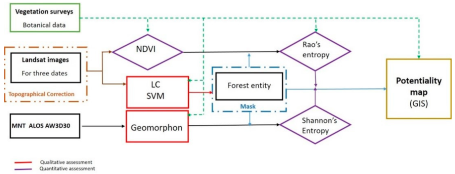
2. Materials and Methods
2.1. Study Area
2.2. Phytoecological Data
2.3. LANDSAT Images and Topographic Correction
2.4. Supervised Support Vector Machine Classification
2.5. Classification of Landforms Using the Geomorphon Method
2.6. Normalized Difference Vegetation Index (NDVI)
2.7. Rao’s Quadratic Entropy
2.8. Topographic Landscape Diversity: Shannon Entropy of Geomorphon Classes
2.9. Potential Ecosystem Services Favorability Map
3. Results
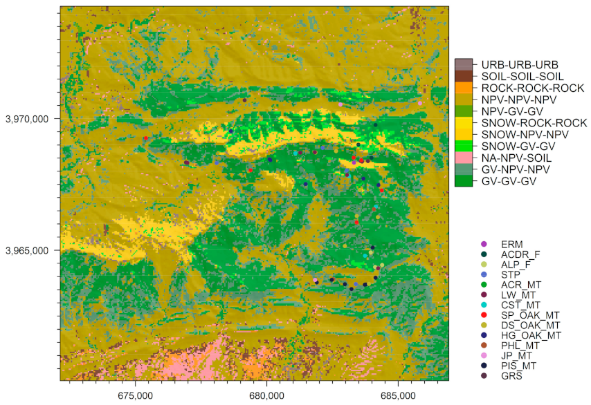
3.1. Land Cover
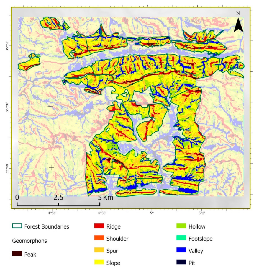
3.2. Geomorphons
3.3. Normalized Difference Vegetation Index (NDVI)
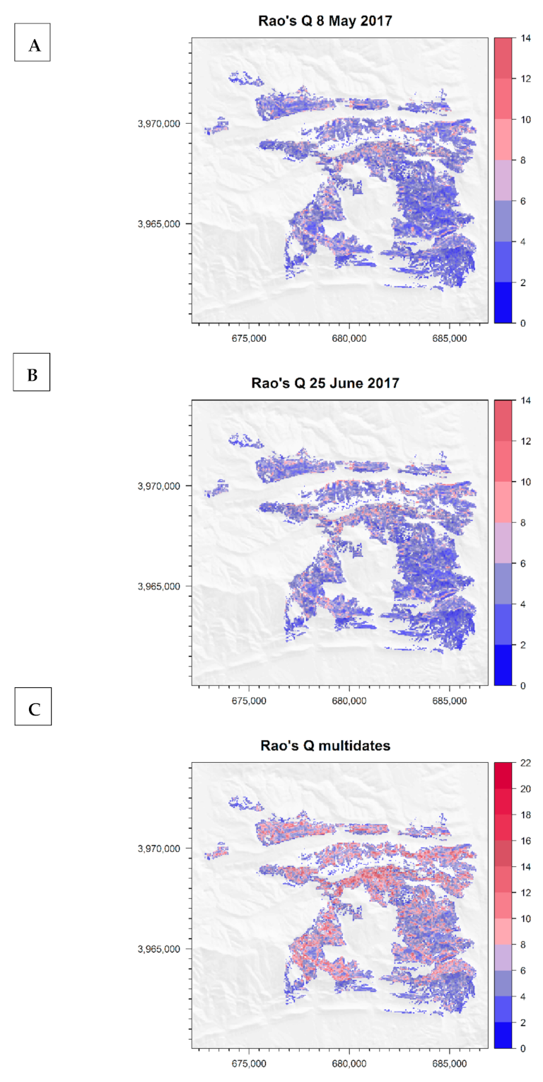
3.4. Rao’s Quadratic Entropy
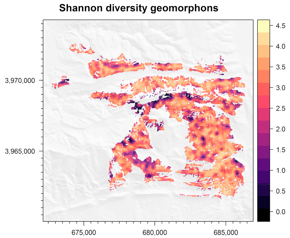
3.5. Shannon Entropy of Geomorphon Classes
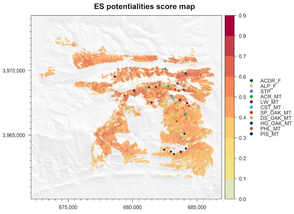
3.6. Ecosystem Services Supply Potentiality Map
4. Discussion and Conclusions
Author Contributions
Funding
Data Availability Statement
Acknowledgments
Conflicts of Interest
References
- Mooney, H.A.; Cropper, A.; Reid, W. The Millennium Ecosystem Assessment: What Is It All About? Trends Ecol. Evol. 2004, 19, 221–224. [Google Scholar] [CrossRef] [PubMed]
- Mainka, S.; McNeely, J.; Jackson, B.; McNeely, J.A. Depend on Nature: Ecosystem Services Supporting Human Livelihoods; IUCN: Grand, Switzerland, 2005. [Google Scholar]
- Viviroli, D.; Weingartner, R.; Messerli, B. Assessing the Hydrological Significance of the World’s Mountains. Mt. Res. Dev. 2003, 23, 32–40. [Google Scholar] [CrossRef] [Green Version]
- Grêt-Regamey, A.; Brunner, S.H.; Kienast, F. Mountain Ecosystem Services: Who Cares? Mt. Res. Dev. 2012, 32 (Suppl. 1), S23–S34. [Google Scholar] [CrossRef]
- Payne, D.; Spehn, E.M.; Snethlage, M.; Fischer, M. Opportunities for Research on Mountain Biodiversity under Global Change. Curr. Opin. Environ. Sustain. 2017, 29, 40–47. [Google Scholar] [CrossRef]
- Grêt-Regamey, A.; Weibel, B. Global Assessment of Mountain Ecosystem Services Using Earth Observation Data. Ecosyst. Serv. 2020, 46, 101213. [Google Scholar] [CrossRef]
- Schirpke, U.; Scolozzi, R.; Dean, G.; Haller, A.; Jäger, H.; Kister, J.; Kovács, B.; Sarmiento, F.O.; Sattler, B.; Schleyer, C. Cultural Ecosystem Services in Mountain Regions: Conceptualising Conflicts among Users and Limitations of Use. Ecosyst. Serv. 2020, 46, 101210. [Google Scholar] [CrossRef]
- Cudlín, P.; Seják, J.; Pokorný, J.; Albrechtová, J.; Bastian, O.; Marek, M. Chapter 24—Forest Ecosystem Services Under Climate Change and Air Pollution. In Developments in Environmental Science; Matyssek, R., Clarke, N., Cudlin, P., Mikkelsen, T.N., Tuovinen, J.-P., Wieser, G., Paoletti, E., Eds.; Climate Change, Air Pollution and Global Challenges; Elsevier: Amsterdam, The Netherlands, 2013; Volume 13, pp. 521–546. [Google Scholar] [CrossRef]
- Masiero, M.; Pettenella, D.; Boscolo, M.; Kanti Barua, S.; Animon, I.; Matta, R. Valuing Forest Ecosystem Services: A Training Manual for Planners and Project Developers; Forestry Working Paper; Food and Agriculture Organization of The United Nations: Rome, Italy, 2019; p. 216. [Google Scholar]
- Ten Brink, P. The Economics of Ecosystems and Biodiversity in National and International Policy Making; Taylor & Francis: Abingdon, UK, 2011; p. 390. [Google Scholar]
- Évaluation des Ressources Forestières Mondiales 2020; FAO: Rome, Italy, 2020. [CrossRef]
- De Groot, R.S.; Wilson, M.A.; Boumans, R.M.J. A Typology for the Classification, Description and Valuation of Ecosystem Functions, Goods and Services. Ecol. Econ. 2002, 41, 393–408. [Google Scholar] [CrossRef] [Green Version]
- Dixon, R.K.; Solomon, A.M.; Brown, S.; Houghton, R.A.; Trexier, M.C.; Wisniewski, J. Carbon Pools and Flux of Global Forest Ecosystems. Science 1994, 263, 185–190. [Google Scholar] [CrossRef]
- Stocker, T. (Ed.) Climate Change 2013: The Physical Science Basis: Working Group I Contribution to the Fifth Assessment Report of the Intergovernmental Panel on Climate Change; Cambridge University Press: Cambridge, UK, 2014. [Google Scholar]
- Palahí, M.; Birot, Y.; Borges, J.G.; Bravo, F.; Pettenella, D.; Sabir, M.; Hassen, H.D.; Shater, Z.; Başkent, E.Z.; Kazana, V. A Mediterranean Forest Research Agenda—MFRA 2010–2020. European Forest Institute. Mediterranean Regional Forest Office–EFIMED. 2009. Available online: https://efi.int/sites/default/files/images/publications/Mediterranean%20Forest%20Research%20Agenda%202010-2020_.pdf (accessed on 7 February 2022).
- Blondel, J. La Production Durable de Biens et Services en Forêt Méditerranéenne: Le Point de Vue de L’écologue. Méditerranéenne 2009, 30, 133–138. Available online: http://www.foret-mediterraneenne.org/fr/catalogue/id-1178-la-production-durable-de-biens-et-services-en-foret-mediterraneenne-le-point-de-vue-de-l-ecologue (accessed on 2 April 2019).
- Anaya-Romero, M.; Muñoz-Rojas, M.; Ibáñez, B.; Marañón, T. Evaluation of Forest Ecosystem Services in Mediterranean Areas. A Regional Case Study in South Spain. Ecosyst. Serv. 2016, 20, 82–90. [Google Scholar] [CrossRef]
- Lovrić, M.; Da Re, R.; Vidale, E.; Prokofieva, I.; Wong, J.; Pettenella, D.; Verkerk, P.J.; Mavsar, R. Collection and Consumption of Non-Wood Forest Products in Europe. For. Int. J. For. Res. 2021, 94, 757–770. [Google Scholar] [CrossRef]
- Nocentini, S.; Travaglini, D.; Muys, B. Managing Mediterranean Forests for Multiple Ecosystem Services: Research Progress and Knowledge Gaps. Curr. For. Rep. 2022, 8, 229–256. [Google Scholar] [CrossRef]
- Benayas, J.M.R.; Newton, A.C.; Diaz, A.; Bullock, J.M. Enhancement of Biodiversity and Ecosystem Services by Ecological Restoration: A Meta-Analysis. Science 2009, 325, 1121–1124. [Google Scholar] [CrossRef] [PubMed]
- Assessment, M.E. Ecosystems and Human Well-Being: Wetlands and Water Synthesis; World Resources Institute: Washington, DC, USA, 2005. [Google Scholar]
- Médail, F.; Quezél, P. Biodiversity Hotspots in the Mediterranean Basin: Setting Global Conservation Priorities. Conserv. Biol. 1999, 13, 1510–1513. [Google Scholar] [CrossRef]
- Tatar, H. Production forestière, exploitation et valorisation en Algérie. Méditerranéenne 2012, 33, 361–368. [Google Scholar]
- Maire, M.; Garavaglia, V.; Picard, N. Maximize the Production of Goods and Services of Mediterranean Forest Ecosystems in the Context of Global Changes; FAO/Plan Bleu: Rome, Italy, 2016; Available online: https://www.fao.org/3/i5887e/i5887e.pdf (accessed on 7 February 2022).
- Khaznadar, M. Etude et Cartographie des Services Ecosystémiques du Parc National d’El Kala (Algérie). Ph.D. Thesis, Ferhat Abbes Sétif 1 University, Sétif, Algeria, 2016. [Google Scholar]
- Luck, G.W.; Harrington, R.; Harrison, P.A.; Kremen, C.; Berry, P.M.; Bugter, R.; Dawson, T.P.; de Bello, F.; Díaz, S.; Feld, C.K.; et al. Quantifying the Contribution of Organisms to the Provision of Ecosystem Services. BioScience 2009, 59, 223–235. [Google Scholar] [CrossRef]
- Andrew, M.E.; Wulder, M.A.; Nelson, T.A. Potential Contributions of Remote Sensing to Ecosystem Service Assessments. Prog. Phys. Geogr. Earth Environ. 2014, 38, 328–353. [Google Scholar] [CrossRef] [Green Version]
- Andrew, M.E.; Wulder, M.A.; Nelson, T.A.; Coops, N.C. Spatial Data, Analysis Approaches, and Information Needs for Spatial Ecosystem Service Assessments: A Review. GIScience Remote Sens. 2015, 52, 344–373. [Google Scholar] [CrossRef] [Green Version]
- Skidmore, A.K.; Pettorelli, N.; Coops, N.C.; Geller, G.N.; Hansen, M.; Lucas, R.; Mücher, C.A.; O’Connor, B.; Paganini, M.; Pereira, H.M.; et al. Environmental Science: Agree on Biodiversity Metrics to Track from Space. Nature 2015, 523, 403–405. [Google Scholar] [CrossRef] [Green Version]
- Ayanu, Y.Z.; Conrad, C.; Nauss, T.; Wegmann, M.; Koellner, T. Quantifying and Mapping Ecosystem Services Supplies and Demands: A Review of Remote Sensing Applications. Environ. Sci. Technol. 2012, 46, 8529–8541. [Google Scholar] [CrossRef]
- Cord, A.F.; Brauman, K.A.; Chaplin-Kramer, R.; Huth, A.; Ziv, G.; Seppelt, R. Priorities to Advance Monitoring of Ecosystem Services Using Earth Observation. Trends Ecol. Evol. 2017, 32, 416–428. [Google Scholar] [CrossRef]
- Burkhard, B.; Kroll, F.; Müller, F.; Windhorst, W. Landscapes’ Capacities to Provide Ecosystem Services—A Concept for Land-Cover Based Assessments. Landsc. Online 2009, 15, 22. [Google Scholar] [CrossRef]
- Syrbe, R.-U.; Walz, U. Spatial Indicators for the Assessment of Ecosystem Services: Providing, Benefiting and Connecting Areas and Landscape Metrics. Ecol. Indic. 2012, 21, 80–88. [Google Scholar] [CrossRef]
- Lausch, A.; Schaepman, M.E.; Skidmore, A.K.; Catana, E.; Bannehr, L.; Bastian, O.; Borg, E.; Bumberger, J.; Dietrich, P.; Glässer, C.; et al. Remote Sensing of Geomorphodiversity Linked to Biodiversity—Part III: Traits, Processes and Remote Sensing Characteristics. Remote Sens. 2022, 14, 2279. [Google Scholar] [CrossRef]
- Abelleira Martínez, O.J.; Fremier, A.K.; Günter, S.; Ramos Bendaña, Z.; Vierling, L.; Galbraith, S.M.; Bosque-Pérez, N.A.; Ordoñez, J.C. Scaling up Functional Traits for Ecosystem Services with Remote Sensing: Concepts and Methods. Ecol. Evol. 2016, 6, 4359–4371. [Google Scholar] [CrossRef] [PubMed]
- Shen, J.; Chen, C.; Wang, Y. What Are the Appropriate Mapping Units for Ecosystem Service Assessments? A Systematic Review. Ecosyst. Health Sustain. 2021, 7, 1888655. [Google Scholar] [CrossRef]
- Pettorelli, N.; Schulte to Bühne, H.; Tulloch, A.; Dubois, G.; Macinnis-Ng, C.; Queirós, A.M.; Keith, D.A.; Wegmann, M.; Schrodt, F.; Stellmes, M.; et al. Satellite Remote Sensing of Ecosystem Functions: Opportunities, Challenges and Way Forward. Remote Sens. Ecol. Conserv. 2018, 4, 71–93. [Google Scholar] [CrossRef]
- Hooper, D.U.; Chapin, F.S., III; Ewel, J.J.; Hector, A.; Inchausti, P.; Lavorel, S.; Lawton, J.H.; Lodge, D.M.; Loreau, M.; Naeem, S.; et al. Effects of Biodiversity on Ecosystem Functioning: A Consensus of Current Knowledge. Ecol. Monogr. 2005, 75, 3–35. [Google Scholar] [CrossRef]
- de Bello, F.; Lavorel, S.; Díaz, S.; Harrington, R.; Cornelissen, J.H.C.; Bardgett, R.D.; Berg, M.P.; Cipriotti, P.; Feld, C.K.; Hering, D.; et al. Towards an Assessment of Multiple Ecosystem Processes and Services via Functional Traits. Biodivers Conserv. 2010, 19, 2873–2893. [Google Scholar] [CrossRef]
- Lausch, A.; Erasmi, S.; King, D.J.; Magdon, P.; Heurich, M. Understanding Forest Health with Remote Sensing -Part I—A Review of Spectral Traits, Processes and Remote-Sensing Characteristics. Remote Sens. 2016, 8, 1029. [Google Scholar] [CrossRef] [Green Version]
- Kc, A.; Wagle, N.; Acharya, T.D. Spatiotemporal Analysis of Land Cover and the Effects on Ecosystem Service Values in Rupandehi, Nepal from 2005 to 2020. ISPRS Int. J. Geo-Inf. 2021, 10, 635. [Google Scholar] [CrossRef]
- Bord, J.P. Cartographie de L’utilisation du sol dans l’Est Algérien: Essai de Zonage Agricole. Ph.D. Thesis, Université Paul Valéry-Montpellier III, Montpellier, France, 1981. [Google Scholar]
- Bureau National d’Études pour le Développement Rural (BNEDER). Etude D’aménagement et de Développement de la Forêt Domaniale de Ouled Hanneche Dans la Wilaya de Bordj Bou Arréridj; Bureau National d’Études pour le Développement Rural (BNEDER): Chéraga, Algérie, 2010.
- Louail, A.; Messner, F.; Missaoui, K.; Djellouli, Y.; Gharzouli, R. Evolution of Local Bioclimates Facing Climate Change in Algeria: Mapping by Global Bioclimatic Classification and Clustering Method. In Proceedings of the International Society for Ecological Modelling Global Conference, Salzburg, Austria, 30 September–4 October 2019. [Google Scholar]
- Official Journal of the Algerian Republic (JORA). N°03. 18-01-2012. Executive Decree No. 12-03 of 10 Safar 1433 Corresponding to January 4, 2012 Establishing the List of Protected Non-Crop Species. 2012, p. 44. Available online: https://gazettes.africa/archive/dz/2012/dz-government-gazette-dated-2012-01-18-no-3.pdf (accessed on 21 June 2021).
- Atbib, M. Etude phytoécologique de la réserve biologique de Mehdia (Littoral Atlantique du Maroc). 1ère partie-La végétation hygrophile de la merja Sidi Bou Ghaba. Bull. L’institut Sci. 1980, 4, 112. [Google Scholar]
- Masek, J.G.; Vermote, E.F.; Saleous, N.; Wolfe, R.; Hall, F.G.; Huemmrich, K.F.; Gao, F.; Kutler, J.; Lim, T.K. LEDAPS Landsat Calibration, Reflectance, Atmospheric Correction Preprocessing Code; ORNL DAAC: Oak Ridge, TN, USA, 2012. [Google Scholar] [CrossRef]
- Sola, I.; González-Audícana, M.; Álvarez-Mozos, J. The Added Value of Stratified Topographic Correction of Multispectral Images. Remote Sens. 2016, 8, 131. [Google Scholar] [CrossRef] [Green Version]
- Hantson, S.; Chuvieco, E. Evaluation of Different Topographic Correction Methods for Landsat Imagery. Int. J. Appl. Earth Obs. Geoinf. 2011, 13, 691–700. [Google Scholar] [CrossRef]
- Sola, I.; González-Audícana, M.; Álvarez-Mozos, J. Multi-Criteria Evaluation of Topographic Correction Methods. Remote Sens. Environ. 2016, 184, 247–262. [Google Scholar] [CrossRef] [Green Version]
- Soenen, S.A.; Peddle, D.R.; Coburn, C.A. SCS + C: A Modified Sun-Canopy-Sensor Topographic Correction in Forested Terrain. IEEE Trans. Geosci. Remote Sens. 2005, 43, 2148–2159. [Google Scholar] [CrossRef]
- Vázquez-Jiménez, R.; Romero-Calcerrada, R.; Ramos-Bernal, R.N.; Arrogante-Funes, P.; Novillo, C.J. Topographic Correction to Landsat Imagery through Slope Classification by Applying the SCS + C Method in Mountainous Forest Areas. ISPRS Int. J. Geo-Inf. 2017, 6, 287. [Google Scholar] [CrossRef]
- Mountrakis, G.; Im, J.; Ogole, C. Support Vector Machines in Remote Sensing: A Review. ISPRS J. Photogramm. Remote Sens. 2011, 66, 247–259. [Google Scholar] [CrossRef]
- Roberts, D.A.; Gardner, M.; Church, R.; Ustin, S.; Scheer, G.; Green, R.O. Mapping Chaparral in the Santa Monica Mountains Using Multiple Endmember Spectral Mixture Models. Remote Sens. Environ. 1998, 65, 267–279. [Google Scholar] [CrossRef]
- Jasiewicz, J.; Stepinski, T.F. Geomorphons—A Pattern Recognition Approach to Classification and Mapping of Landforms. Geomorphology 2013, 182, 147–156. [Google Scholar] [CrossRef]
- Tadono, T.; Nagai, H.; Ishida, H.; Oda, F.; Naito, S.; Minakawa, K.; Iwamoto, H. Generation of the 30 M-mesh global digital surface model by ALOS PRISM. Int. Arch. Photogramm. Remote Sens. Spat. Inf. Sci. 2016, 41, 157–162. [Google Scholar]
- Rouse, J.W.; Haas, R.H.; Schell, J.A.; Deering, D.W. Monitoring Vegetation Systems in the Great Plains with ERTS. In Proceedings of the 3rd ERTS Symposium, NASA SP-351, Washington, DC, USA, 10–14 December 1973; pp. 309–317. [Google Scholar]
- Tucker, C.J.; Townshend, J.R.G.; Goff, T.E. African Land-Cover Classification Using Satellite Data. Science 1985, 227, 369–375. [Google Scholar] [CrossRef] [PubMed]
- Wegmann, M.; Leutner, B.; Dech, S. Remote Sensing and GIS for Ecologists: Using Open Source Software; Exeter Pelagic Publishing Ltd.: Exeter, UK, 2016; p. 352. [Google Scholar]
- Pettorelli, N. The Normalized Difference Vegetation Index, 1st ed.; Oxford University Press: Oxford, UK, 2013; p. 194. [Google Scholar]
- Krishnaswamy, J.; Bawa, K.S.; Ganeshaiah, K.N.; Kiran, M.C. Quantifying and Mapping Biodiversity and Ecosystem Services: Utility of a Multi-Season NDVI Based Mahalanobis Distance Surrogate. Remote Sens. Environ. 2009, 113, 857–867. [Google Scholar] [CrossRef]
- Paruelo, J.M.; Texeira, M.; Staiano, L.; Mastrángelo, M.; Amdan, L.; Gallego, F. An Integrative Index of Ecosystem Services Provision Based on Remotely Sensed Data. Ecol. Indic. 2016, 71, 145–154. [Google Scholar] [CrossRef] [Green Version]
- Jullian, C.; Nahuelhual, L.; Laterra, P. The Ecosystem Service Provision Index as a Generic Indicator of Ecosystem Service Supply for Monitoring Conservation Targets. Ecol. Indic. 2021, 129, 107855. [Google Scholar] [CrossRef]
- Rocchini, D.; Salvatori, N.; Beierkuhnlein, C.; Chiarucci, A.; de Boissieu, F.; Förster, M.; Garzon-Lopez, C.X.; Gillespie, T.W.; Hauffe, H.C.; He, K.S.; et al. From Local Spectral Species to Global Spectral Communities: A Benchmark for Ecosystem Diversity Estimate by Remote Sensing. Ecol. Inform. 2021, 61, 101195. [Google Scholar] [CrossRef]
- Gillespie, T.W.; Foody, G.M.; Rocchini, D.; Giorgi, A.P.; Saatchi, S. Measuring and Modelling Biodiversity from Space. Prog. Phys. Geogr. Earth Environ. 2008, 32, 203–221. [Google Scholar] [CrossRef]
- Boyd, D.S.; Foody, G.M. An Overview of Recent Remote Sensing and GIS Based Research in Ecological Informatics. Ecol. Inform. 2011, 6, 25–36. [Google Scholar] [CrossRef] [Green Version]
- Palmer, M.W.; Earls, P.G.; Hoagland, B.W.; White, P.S.; Wohlgemuth, T. Quantitative Tools for Perfecting Species Lists. Environmetrics 2002, 13, 121–137. [Google Scholar] [CrossRef]
- Shannon, C.E. A Mathematical Theory of Communication. Bell Syst. Tech. J. 1948, 27, 379–423. [Google Scholar] [CrossRef] [Green Version]
- Rocchini, D.; Marcantonio, M.; Ricotta, C. Measuring Rao’s Q Diversity Index from Remote Sensing: An Open Source Solution. Ecol. Indic. 2017, 72, 234–238. [Google Scholar] [CrossRef]
- Rao, C.R. Diversity and Dissimilarity Coefficients: A Unified Approach. Theor. Popul. Biol. 1982, 21, 24–43. [Google Scholar] [CrossRef]
- Botta-Dukát, Z. Rao’s Quadratic Entropy as a Measure of Functional Diversity Based on Multiple Traits. J. Veg. Sci. 2005, 16, 533–540. [Google Scholar] [CrossRef]
- Thouverai, E.; Marcantonio, M.; Bacaro, G.; Re, D.D.; Iannacito, M.; Marchetto, E.; Ricotta, C.; Tattoni, C.; Vicario, S.; Rocchini, D. Measuring Diversity from Space: A Global View of the Free and Open Source Rasterdiv R Package under a Coding Perspective. Community Ecol. 2021, 22, 1–11. [Google Scholar] [CrossRef]
- Amatulli, G.; Domisch, S.; Tuanmu, M.-N.; Parmentier, B.; Ranipeta, A.; Malczyk, J.; Jetz, W. A Suite of Global, Cross-Scale Topographic Variables for Environmental and Biodiversity Modeling. Sci Data 2018, 5, 180040. [Google Scholar] [CrossRef] [Green Version]
- Doxa, A.; Prastacos, P. Using Rao’s Quadratic Entropy to Define Environmental Heterogeneity Priority Areas in the European Mediterranean Biome. Biol. Conserv. 2020, 241, 108366. [Google Scholar] [CrossRef]
- Malczewski, J. Multicriteria Analysis. In Comprehensive Geographic Information Systems; Elsevier: Amsterdam, The Netherlands, 2018; pp. 197–217. [Google Scholar] [CrossRef]
- Evans, J.S. Spatialeco. R Package Version 1.3-6. 2021. Available online: https://github.com/jeffreyevans/spatialEco (accessed on 6 May 2022).
- Malczewski, J. On the Use of Weighted Linear Combination Method in GIS: Common and Best Practice Approaches. Trans. GIS 2000, 4, 5–22. [Google Scholar] [CrossRef]
- Saaty, T.L. The Analytic Hierarchy Process: Planning, Priority Setting, Resource Allocation; McGraw-Hill International Book Co.: New York, NY, USA; London, UK, 1980. [Google Scholar]
- Saaty, T.L. Decision Making—The Analytic Hierarchy and Network Processes (AHP/ANP). J. Syst. Sci. Syst. Eng. 2004, 13, 1–35. [Google Scholar] [CrossRef]
- Cho, H.T.F. Analytic Hierarchy Process for Survey Data in R (Vignettes). 2018. Available online: https://doi.org/10.13140/RG.2.2.25278.13125 (accessed on 6 May 2022).
- Sirvent, L. Les Types Biologiques: État de L’art, Actualisation des Définitions et Mise en Place d’un Référentiel. 2020. Available online: https://doi.org/10.13140/RG.2.2.14673.89440 (accessed on 6 February 2022).
- Stein, A.; Kreft, H. Terminology and Quantification of Environmental Heterogeneity in Species-Richness Research. Biol. Rev. 2014, 90, 815–836. [Google Scholar] [CrossRef]
- Badgley, C.; Smiley, T.M.; Terry, R.; Davis, E.B.; DeSantis, L.R.G.; Fox, D.L.; Hopkins, S.S.B.; Jezkova, T.; Matocq, M.D.; Matzke, N.; et al. Biodiversity and Topographic Complexity: Modern and Geohistorical Perspectives. Trends Ecol. Evol. 2017, 32, 211–226. [Google Scholar] [CrossRef] [Green Version]
- Rocchini, D.; Luque, S.; Pettorelli, N.; Bastin, L.; Doktor, D.; Faedi, N.; Feilhauer, H.; Féret, J.-B.; Foody, G.M.; Gavish, Y.; et al. Measuring β-Diversity by Remote Sensing: A Challenge for Biodiversity Monitoring. Methods Ecol. Evol. 2018, 9, 1787–1798. [Google Scholar] [CrossRef] [Green Version]
- Khare, S.; Latifi, H.; Rossi, S. Forest Beta-Diversity Analysis by Remote Sensing: How Scale and Sensors Affect the Rao’s Q Index. Ecol. Indic. 2019, 106, 105520. [Google Scholar] [CrossRef]
- Lausch, A.; Bannehr, L.; Beckmann, M.; Boehm, C.; Feilhauer, H.; Hacker, J.M.; Heurich, M.; Jung, A.; Klenke, R.; Neumann, C.; et al. Linking Earth Observation and Taxonomic, Structural and Functional Biodiversity: Local to Ecosystem Perspectives. Ecol. Indic. 2016, 70, 317–339. [Google Scholar] [CrossRef]
- Regos, A.; Gonçalves, J.; Arenas-Castro, S.; Alcaraz-Segura, D.; Guisan, A.; Honrado, J.P. Mainstreaming Remotely Sensed Ecosystem Functioning in Ecological Niche Models. Remote Sens. Ecol. Conserv. 2022. [Google Scholar] [CrossRef]
- Wulder, M.A.; Coops, N.C. Satellites: Make Earth Observations Open Access. Nature 2014, 513, 30–31. [Google Scholar] [CrossRef] [PubMed]
- Baret, F.; Guyot, G. Potentials and Limits of Vegetation Indices for LAI and APAR Assessment. Remote Sens. Environ. 1991, 35, 161–173. [Google Scholar] [CrossRef]
- Baret, F.; Buis, S. Estimating Canopy Characteristics from Remote Sensing Observations: Review of Methods and Associated Problems. In Advances in Land Remote Sensing: System, Modeling, Inversion and Application; Liang, S., Ed.; Springer: Dordrecht, The Netherlands, 2008; pp. 173–201. [Google Scholar] [CrossRef]
- Jacquemoud, S.; Verhoef, W.; Baret, F.; Bacour, C.; Zarco-Tejada, P.J.; Asner, G.P.; François, C.; Ustin, S.L. PROSPECT+SAIL Models: A Review of Use for Vegetation Characterization. Remote Sens. Environ. 2009, 113, S56–S66. [Google Scholar] [CrossRef]
- Berger, K.; Atzberger, C.; Danner, M.; D’Urso, G.; Mauser, W.; Vuolo, F.; Hank, T. Evaluation of the PROSAIL Model Capabilities for Future Hyperspectral Model Environments: A Review Study. Remote Sens. 2018, 10, 85. [Google Scholar] [CrossRef] [Green Version]
- Weiss, M.; Baret, F. S2toolbox Level 2 Products: Lai, Fapar, Fcover; Institut National de la Recherche Agronomique (INRA): Avignon, France, 2016. [Google Scholar]
- Malczewski, J.; Jankowski, P. Emerging Trends and Research Frontiers in Spatial Multicriteria Analysis. Int. J. Geogr. Inf. Sci. 2020, 34, 1257–1282. [Google Scholar] [CrossRef]
- Baskent, E.Z.; Borges, J.G.; Kašpar, J.; Tahri, M. A Design for Addressing Multiple Ecosystem Services in Forest Management Planning. Forests 2020, 11, 1108. [Google Scholar] [CrossRef]
- Landuyt, D.; Broekx, S.; D’hondt, R.; Engelen, G.; Aertsens, J.; Goethals, P.L.M. A Review of Bayesian Belief Networks in Ecosystem Service Modelling. Environ. Model. Softw. 2013, 46, 1–11. [Google Scholar] [CrossRef]


| 17 February | 8 May | 25 June | 3 Dates | |
|---|---|---|---|---|
| Model | SVM radial basis | SVM radial basis | SVM radial basis | SVM radial basis |
| Number of training samples | 237 | 237 | 237 | 237 |
| Number of predictors | 7 | 7 | 7 | 21 |
| Number of classes | 7 | 6 | 6 | 10 |
| Model evaluation | repeated K-fold CV | repeated K-fold CV | repeated K-fold CV | repeated K-fold CV |
| Number K-fold | 10 | 10 | 10 | 10 |
| Number repetition | 10 | 10 | 10 | 10 |
| Best sigma parameter | 0.2 | 1 | 0.5 | 0.5 |
| Best C parameter | 0.1 | 1.25 | 15 | 0.9 |
| Overall accuracy | 0.66 | 0.76 | 0.78 | 0.63 |
| Kappa | 0.53 | 0.68 | 0.68 | 0.55 |
| Diversity Geomorphon | Rao Entropy | Mean NDVI | |
|---|---|---|---|
| Diversity geomorphon | 1 | 0.5 | 0.25 |
| Rao entropy | 2 | 1 | 0.33 |
| Mean NDVI | 4 | 3 | 1 |
| Diversity Geomorphon | Rao Entropy | Mean NDVI |
|---|---|---|
| 0.136 | 0.238 | 0.625 |
| CR | 0.017 |
| Plant Species | R | Plant Species | R | Plant Species | R |
|---|---|---|---|---|---|
| Quercus ilex | 42/68 | Rosa canina | 15/68 | Pinus halepensis | 9/68 |
| Juniperus oxycedrus | 29/68 | Globularia alypum | 14/68 | Rhamnus lycioides | 9/68 |
| Juniperus phoenicea | 27/68 | Cedrus atlantica | 13/68 | Pistacia atlantica | 8/68 |
| Cistus albidus | 26/68 | Genista microcephala | 12/68 | Thapsia garganica | 7/68 |
| Pistacia lentiscus | 20/68 | Astragalus sp. | 12/68 | Lonicera impelaxa | 7/68 |
| Ampelodesmos mauritanicus | 19/68 | Jasminum fruticans | 11/68 | Teucrium polium | 7/68 |
| Phillyrea angustifolia | 18/68 | Crataegus monogyna | 11/68 | Bunium sp. | 6/68 |
| Santolina rosmarinifolia | 17/68 | Rosmarinus officinalis | 10/68 | Bupleurum sp. | 6/68 |
| Stipa tenacissima | 16/68 | Galium sp. | 9/68 | Eryngium sp. | 6/68 |
| Acer monspessulanum | 16/68 | Crataegus azarolus | 9/68 | Lomelosia stellata | 6/68 |
| Calicotome spinosa | 15/68 | Asparagus acutifolius | 9/68 | Aegilops geniculata | 6/68 |
Publisher’s Note: MDPI stays neutral with regard to jurisdictional claims in published maps and institutional affiliations. |
© 2022 by the authors. Licensee MDPI, Basel, Switzerland. This article is an open access article distributed under the terms and conditions of the Creative Commons Attribution (CC BY) license (https://creativecommons.org/licenses/by/4.0/).
Share and Cite
Louail, A.; Messner, F.; Djellouli, Y.; Gharzouli, R. Remote Sensing and Phytoecological Methods for Mapping and Assessing Potential Ecosystem Services of the Ouled Hannèche Forest in the Hodna Mountains, Algeria. Forests 2022, 13, 1159. https://doi.org/10.3390/f13081159
Louail A, Messner F, Djellouli Y, Gharzouli R. Remote Sensing and Phytoecological Methods for Mapping and Assessing Potential Ecosystem Services of the Ouled Hannèche Forest in the Hodna Mountains, Algeria. Forests. 2022; 13(8):1159. https://doi.org/10.3390/f13081159
Chicago/Turabian StyleLouail, Amal, François Messner, Yamna Djellouli, and Rachid Gharzouli. 2022. "Remote Sensing and Phytoecological Methods for Mapping and Assessing Potential Ecosystem Services of the Ouled Hannèche Forest in the Hodna Mountains, Algeria" Forests 13, no. 8: 1159. https://doi.org/10.3390/f13081159
APA StyleLouail, A., Messner, F., Djellouli, Y., & Gharzouli, R. (2022). Remote Sensing and Phytoecological Methods for Mapping and Assessing Potential Ecosystem Services of the Ouled Hannèche Forest in the Hodna Mountains, Algeria. Forests, 13(8), 1159. https://doi.org/10.3390/f13081159