Spatio-Temporal Dynamic Evolution and Simulation of Dike-Pond Landscape and Ecosystem Service Value Based on MCE-CA-Markov: A Case Study of Shunde, Foshan

Abstract

Dike-pond is a unique agricultural landscape type in the Pearl River Delta region of China, which has significance for the maintenance of ecological balance. In recent years, urbanization in China has developed rapidly, and dike-ponds have been extensively occupied, reducing their ecological regulation ability and threatening regional ecological security. Taking the Shunde District of Foshan as an example, based on remote sensing images from 1979 to 2020, using a CA-Markov model with the multi-criteria evaluation method (MCE), firstly the spatial and temporal evolution characteristics of the dike-pond landscape pattern were analyzed, then the dike-pond landscape in 2030 was simulated. At last, the spatio-temporal evolution of ecosystem service value (ESV) in Shunde was visualized. The results show that: (1) In the past four decades, the landscape types in Shunde have changed significantly. This mainly manifested as dike-pond, cultivated land, and forest land transforming into construction land. (2) At the class level, the degree of dike-pond landscape fragmentation increased, and the degree of dominance and agglomeration decreased. At the landscape level, the regional degree of dominance showed an upward trend, whereas the overall landscape showed an unbalanced trend distribution. It is predicted that from 2020 to 2030, the landscape pattern of dike-pond will not change significantly, and the overall landscape richness will increase. (3) The ESV in Shunde decreased continuously from 1979 to 2020. The dike-pond ESV accounts for the largest proportion and is the main landscape type that maintains ecological balance. It is predicted that the ESV decline will slow in the future. (4) The optimized MCE-CA-Markov model has greater precision and produces better simulations. The dike-pond development model proposed in this study can provide a scientific basis for delimiting the scope of regional ecological protection and sustainable development.

1. Introduction

Over the past four decades, China has made great achievements in its economy and urbanization [1]; however, excessive urban expansion and population growth have resulted in large areas of natural land being occupied by construction land, thereby damaging the regional environment [2]. The abundant, spreading Pearl River system nourishes the people of the Pearl River Delta and gives rise to a unique land type, the dike-pond. This is a large area composite agricultural production system composed of fishponds and pond foundations, which promotes the development and prosperity of the agricultural economy in the Pearl River Delta [3,4]. The dike-pond is a natural–artificial composite wetland ecosystem, which is conducive to maintaining the regional ecological balance [4]. After thousands of years of artificial reclamation and natural evolution, dike-ponds have become a unique vernacular landscape [5]. In 2020, the dike-ponds of Foshan, Guangdong were recognized as an important Chinese agricultural cultural heritage site, and the most concentrated area of dike-ponds, “Sangyuanwei”, became a World Irrigation Heritage [6].

Research on dike-ponds was first recorded in The Introduction of Sericulture in Guangdong, in which traditional dike-pond agricultural techniques were analyzed [7]. In the 1980s, Zhong described dike-pond systems as natural–artificial ecosystems, and studied their structure, function, and ecological and economic benefits [8]. Following this, Korn et al. conducted in-depth studies on the ecosystem cycle of dike-pond systems in China [9], and Hill et al. studied the ecological engineering problems of the dike-pond system in the Pearl River Delta and noted the ecological effects of the system [10]. In recent years, with the rapid development of urbanization, the transformation of different land use types in the Pearl River Delta has resulted in significant shrinkage of dike-pond areas; dike-pond landscapes have become fragmented and isolated, and the regional ecological environmental quality has declined [11]. Simultaneously, the agricultural production function of dike-pond systems has been greatly degraded, partially because of modern intensive agriculture [12], which suggests that the dike-pond’s single agricultural production function should be transformed into more ecological and social functions [13]. Research on the ecological environment of dike-ponds in the Pearl River Delta has become a hot topic [14,15]. For example, Ding analyzed the current situation of the dike-pond system in the context of urbanization through field research and found that recycling development of the dike-pond system must be carried out in a sustainable manner [16]. Furthermore, Nie investigated and analyzed the reasons for and mechanism of dike-pond system degradation in Shunde District and proposed a feasible method to restore certain degraded dike-pond systems and apply the principles of food chains and ecological niches [17].

Changes in land use and land cover (LUCC) can change regional landscape patterns, which can affect regional ecological processes and environmental quality [18]. Currently, the evolution and simulation of landscape patterns have been examined at multiple scales, including countries [19,20], regions [21,22], cities [23,24], and counties [25], mostly covering all landscape types in the area. Some focus on particular landscapes, such as watersheds [26,27], forests [28], and wetlands [29]. With the wide application of 3S technology, spatial analysis has been applied to dike-pond research. Using Landsat TM remote sensing image data from 1990, 2000, and 2006, Ye extracted the landscape of dike-ponds in the Pearl River Delta and discussed changes in the spatial patterns. Ye divided the Pearl River Delta into four categories, according to the comprehensive expansion coefficient of the dike-pond: strong expansion, weak expansion, relatively stable, and shrinking [30]. Liu used three remote sensing images from 1988, 1998, and 2006 to analyze the changing spatial patterns of dike-ponds, and then analyzed their spatial evolution in combination with the land use change transfer matrix, which showed that the traditional dike-pond system is gradually dying out in the Pearl River Delta [31]. Han analyzed the changes in dike-pond patterns in Shunde District in the context of rapid urbanization using the landscape index and simulated five “city–dike-pond” landscape ecological security patterns [32].

However, fully capturing and simulating landscape pattern changes remains challenging [33]. In recent years, researchers have attempted to explore the complexity and uncertainty of landscape changes using various models, most often quantitative and spatial simulation models [34]. A quantitative simulation model is based on statistical analysis of variables, including logistic regression statistics [35], system dynamics analysis [36], and Markov chain [37]. Spatial simulations include spatial allocation capability, such as the CA model [38], FLUS model [39], and GeoSOS model [40]. Currently, very few single models can capture all the complex features of landscape pattern changes; therefore, improved models coupled with quantitative and spatial models have become the main trend in studying simulated landscape patterns [41]. The CA-Markov model combines the ability of the CA model to simulate spatial changes within a complex system. It takes advantage of the Markov model for long-term predictions, which can effectively simulate the quantitative and spatial changes in landscape pattern [42]. In addition, the MCE-CA-Markov model uses the multi-criteria evaluation (MCE) method to quantify all influencing factors and supplement the transformation rules of the CA model in order to increase model accuracy [43]. Previous studies mostly considered bottom-up influencing factors, such as natural factors (slope and elevation) and social factors (population and GDP) [44]. Top-down policy factors, such as restricted or prohibited development zones and ecological protection zones are rarely considered. Furthermore, when considering the driving factor of distance from the road, researchers generally consider all levels of road as a single factor [45]; however, different road levels can drive landscape pattern changes to a different extent.

Landscape pattern regulation can change the structure of regional ecosystems and affect ecological processes, thereby changing the service value of an ecosystem [46]. Ecosystem service value (ESV) refers to the products and services obtained by humans directly or indirectly through the structure, processes, and functions of an ecosystem [47]. ESV assessment is important for formulating reasonable regional development strategies, ecological protection policies, and realizing regional sustainable development [48]. Most existing studies focus on ecosystem service classification, quantitative evaluation of value, trade-offs, and synergies [49,50]. Research methods include InVEST model analysis, value scale estimation, and principal component analysis [51]. Dike-pond is recognized as a natural–artificial wetland ecosystem, which is of great significance for maintaining regional ecological stability. The service functions and value of wetland ecosystems, including dike-ponds, is well known [52]. Although some studies focus on the impact of land use change on the ecosystem services of dike-ponds [53], few have examined the change in their ESV from the perspective of landscape pattern evolution.

Therefore, this study selected Shunde District, which has the most concentrated dike-pond landscape in the Pearl River Delta as the study area, to analyze changes in the landscape pattern of dike-ponds over the past four decades (1979–2020), to explore the influence mechanism, and to simulate the landscape pattern in 2030. The spatial and temporal evolution characteristics of the dike-pond landscape pattern at the landscape and class levels were analyzed. Finally, the temporal and spatial evolution characteristics of the ESV were explored. This study provides a theoretical reference for the optimization of dike-ponds in this region and provides a scientific basis for the ecological protection and territorial space planning of the Pearl River Delta.

2. Materials and Methods

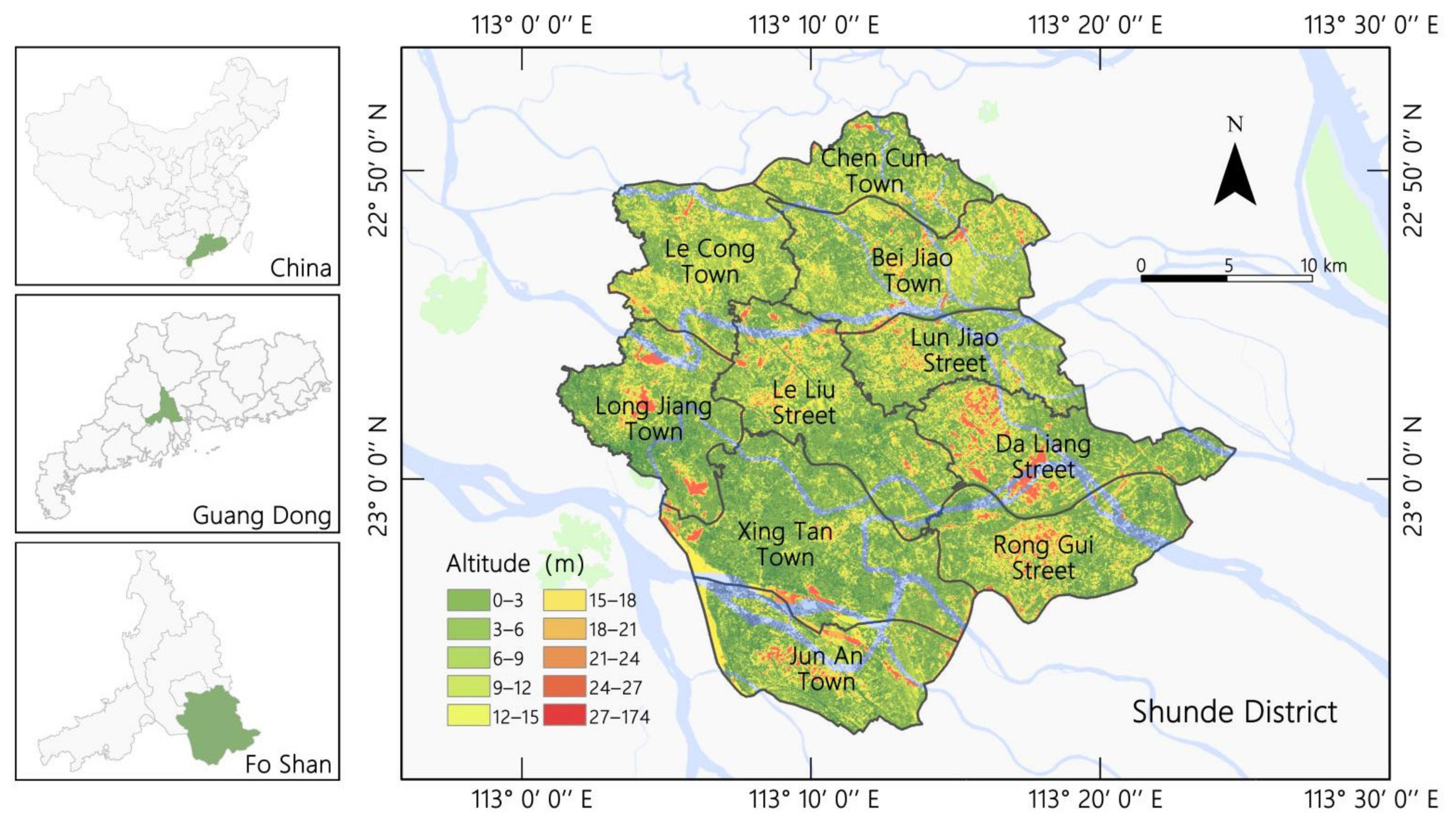
2.1. Study Area

Shunde, Foshan, is located in the middle of the Pearl River Delta estuary plain, south of Guangdong Province in China. It covers 806 km² and has a permanent resident population of approximately 3.22 million, consisting of four streets and seven towns. Most of the study area is located in the south of the Tropic of Cancer and has a south subtropical maritime monsoon climate, so it is always warm and humid, with an annual precipitation of >1600 mm [54]. In addition, most of Shunde District belongs to the estuarine delta plain, which is formed by an alluvial river system. The rivers crisscross one another forming an interwoven water network, and dike-ponds are widely distributed throughout (Figure 1). It has some of the most concentrated and complete dike-pond landscapes in the Pearl River Delta region [55]. Dike-pond agriculture used to be the main source of income for Shunde District residents, and the large areas of dike-ponds maintained the ecological balance of the region. In recent years, with rapid urbanization, the dike-pond areas in Shunde have shrunk, and their production function has been significantly degraded [56]. Therefore, it is necessary to explore the changing pattern of the dike-pond landscape in Shunde and simulate the future landscape pattern of dike-pond.

2.2. Data Source and Preprocessing

The data in this study consisted of five categories: land-use/land-cover (LULC), natural environmental data, socioeconomic data, road distribution data, and local master plan data. LULC data were obtained from supervised classification of Landsat multispectral remote sensing images. First, to avoid the influence of clouds on classification accuracy, five remote sensing images of the study area with <5% cloud cover were downloaded from USGS Earth Explorer (http://www.usgs.gov/ (accessed on 12 December 2020);

Table 1. Remote sensing image information.

Collecting Time	Satellite	Sensor	Spatial Resolution (m)	Path/Row
6 November 1979	Landsat3	MSS	60	131–44
13 October 1990	Landsat5	TM	30	122–44
1 March 2001	Landsat5	TM	30	122–44
6 March 2010	Landsat5	TM	30	122–44
18 February 2020	Landsat8	OLI	30	122–44

). TM images from 2001 and 2010 as well as OLI images from 2020 were collected from the pre-monsoon period. Since the MSS and TM images from 1990 have no pre-monsoon data with <5% cloud cover, the post-monsoon images were used, and we checked that the study area was less affected by monsoons in 1979 and 1990, according to The Shunde Statistical Yearbook. However, the MSS image resolution was 60 m, so it was resampled. Potential resampling methods included nearest-neighbor interpolation, bilinear interpolation, and cubic convolution interpolation. Referring to previous research [57], the nearest neighbor method was chosen to resample the MSS image resolution to 30 m as this scale is efficient, simple, and more suitable for land-use classification. The images were preprocessed for atmospheric correction, radiation correction, and tailoring.

Finally, the Shunde landscape types were divided into dike-pond, forest, water, farmland, construction land, and unused land through SVM supervision classification and visual interpretation, referring to The National Standard of Land Use Classification (GB/T21010-2017) and combining the characteristics of the Shunde landscape type and considering the research purpose and image spatial resolution (

Table 2. Classification and basis of landscape types in the study area.

Serial Number	Landscape Type	Land Use Types and Codes Included
1	Dike-pond	Pit-pond water (1104), Garden (0201–0204)
2	Forest	Woodland (0301–0307), Grassland (0401–0404)
3	Water	Water area (1101–1103, 1105–1108, 1110)
4	Farmland	Farmland (0101–0103)
5	Construction	Commercial service land (0501–0507), Industrial and mining storage land (0601–0604), Residential land (0701–0702), Public management and public service land (0801–0810), Special use of land (0901–0906), Transportation land (1001–1009), Hydraulic construction land (1109), Facility agricultural land (1202),
6	Unused	Other land (1201, 1203, 1204–1207)

). There is little grassland scattered over a large area of forest and a few gardens scattered across a large area of farmland. However, because these scattered grassland and garden patches are too small to be accurately identified and extracted at 30 m spatial resolution, the grassland was categorized as forest and the gardens as arable land. The scattered landscape foundation dike-ponds within the green space on construction land were not extracted separately. For the visual discrimination of remote sensing images with reference to Local Space Viewer, 240 points were randomly sampled to verify the accuracy of the classification. The overall accuracy of the five periods (Table 1) was 90.2, 88.3, 91.7, 92.7, and 92.1%, and the Kappa coefficients were 0.87, 0.84, 0.84, 0.89, 0.90, and 0.90, respectively; the accuracy of the classification results met the requirements.

The natural environmental data included elevation and slope. The elevation was derived from ASTER GDEM 30 m resolution digital data from the Geospatial Data Cloud Platform (http://www.gscloud.cn/ (accessed on 8 December 2020). The slope data were calculated using the Slope Module of ArcGIS 10.8 based on the DEM. The socioeconomic data, including GDP and population, were derived from the WorldPop 100 resolution raster map (https://www.worldpop.org/ (accessed on 22 December 2020) and corrected using The Shunde Statistical Yearbook. The GDP and population data were also resampled using the nearest-neighbor method. Road distribution data were downloaded from the Open Street Map (https://www.openstreetmap.org/ (accessed on 28 December 2020), and the data were classified as railway, highway, primary road, secondary road, tertiary road, and other roads. The local master planning data included prohibited and restricted construction areas, historical protection areas, and built-up areas, which were extracted according to The Master Plan of Shunde District of Foshan City (2009–2020) and The Master Plan of Territorial Space of Foshan City (2020–2035).

2.3. Research Methods

2.3.1. Derivation of Spatial Metrics

Spatial metrics refers to a simple quantitative index that can highly concentrate landscape pattern information, reflecting its structural composition and certain characteristics of spatial configuration [58,59,60]. Based on the principle of landscape ecology, nine spatial metrics were selected using FRAGSTATS (V4.2, Kevin McGarigal & Eduard Ene, Amherst, MA, USA). At the class level, the largest patch index (LPI), mean patch size (MPS), area-weighted mean patch fractal dimension (AWMPFD), and patch cohesion index (COHESION) were calculated. At the landscape level, the number of patches (NP), contagion index (CONTAG), LPI, area-weighted mean patch fractal dimension (AMPFD), and Shannon diversity index (SHDI) were calculated. Details of the spatial metrics are presented in

Table 3. Spatial metrics selected in this study.

Metrics	Abbreviation	Description
Largest Patch Index	LPI	The proportion of total landscape that is made up by the largest patch.
Mean Patch Size	MPS	The area occupied by a particular patch type divided by a number of patches of that type.
Area-Weighted Mean Patch Fractal Dimension	AWMPFD	The sum of the perimeters and area ratios of each patch in a patch type multiplied by the sum of their area weights under the fractal dimension theory.
Patch Cohesion Index	COHESION	It characterizes the connectedness of patches belonging to class i. It can be used to assess if patches of the same class are located aggregated or rather isolated and thereby COHESION gives information about the configuration of the landscape.
Number of Patches	NP	Total number of patches in the landscape.
Contagion Index	CONTAG	The degree of agglomeration or extension of different patch types in the landscape.

.

2.3.2. CA-Markov Model

1.

Cell automata

The cellular automata (CA) model is a dynamic system that is discrete in terms of time and space. A cell is the basic unit of the system. The state of a cell at t + 1 depends on the state of itself and its neighbors at t. The CA model can effectively explain and define spatial variables, plot interactions, and driving forces in the process of landscape change, and represent the state transition rules of cellular unit interactions [61], expressed as follows:

$$C_{(t+1)}=f(S_t,N)$$

(1)

where t and t + 1 are the before and after moments of the cell, C_(t+1) is the state of the cell at time t + 1, f is the cellular transformation rule, S_t is the set of states of the cells at time t, and N is the cell’s neighborhood.

2.

Markov chain

The Markov chain is used to predict the occurrence probability of events based on the Markov process theory. It is often used to predict geographical events without aftereffects. Landscape evolution is a Markov process and landscape types correspond to the “possible state” within the Markov process, while the area and proportion of the transformation between landscape types are the transition probability, which is often expressed as a transition matrix [62]. This is expressed as follows:

$$\begin{array}{c}{T}_{(t+1)}=P_{ij}\times S_t\\ P_{ij}=\left[\begin{array}{cccc}{P}_{11}& P_{12}& \cdots & P_{1n}\\ P_{21}& P_{22}& \cdots & P_{2n}\\ \cdots & \cdots & \cdots & \cdots \\ P_{n1}& P_{n2}& \cdots & P_{nn}\end{array}\right]\end{array}$$

(2)

$$\left(0\le P_{ij}<1, {\displaystyle \sum }_{j=1}^n{P}_{ij}=1\left(i,j=1,2,\cdots ,n\right)\right)$$

(3)

where t and t + 1 are the before and after moments of the landscape type, T_(t+1) is the state at time t + 1, i is the i landscape type, j is the j landscape type, S_t is the state set of landscape types at time t, and P_ij is the transition probability matrix between i and j.

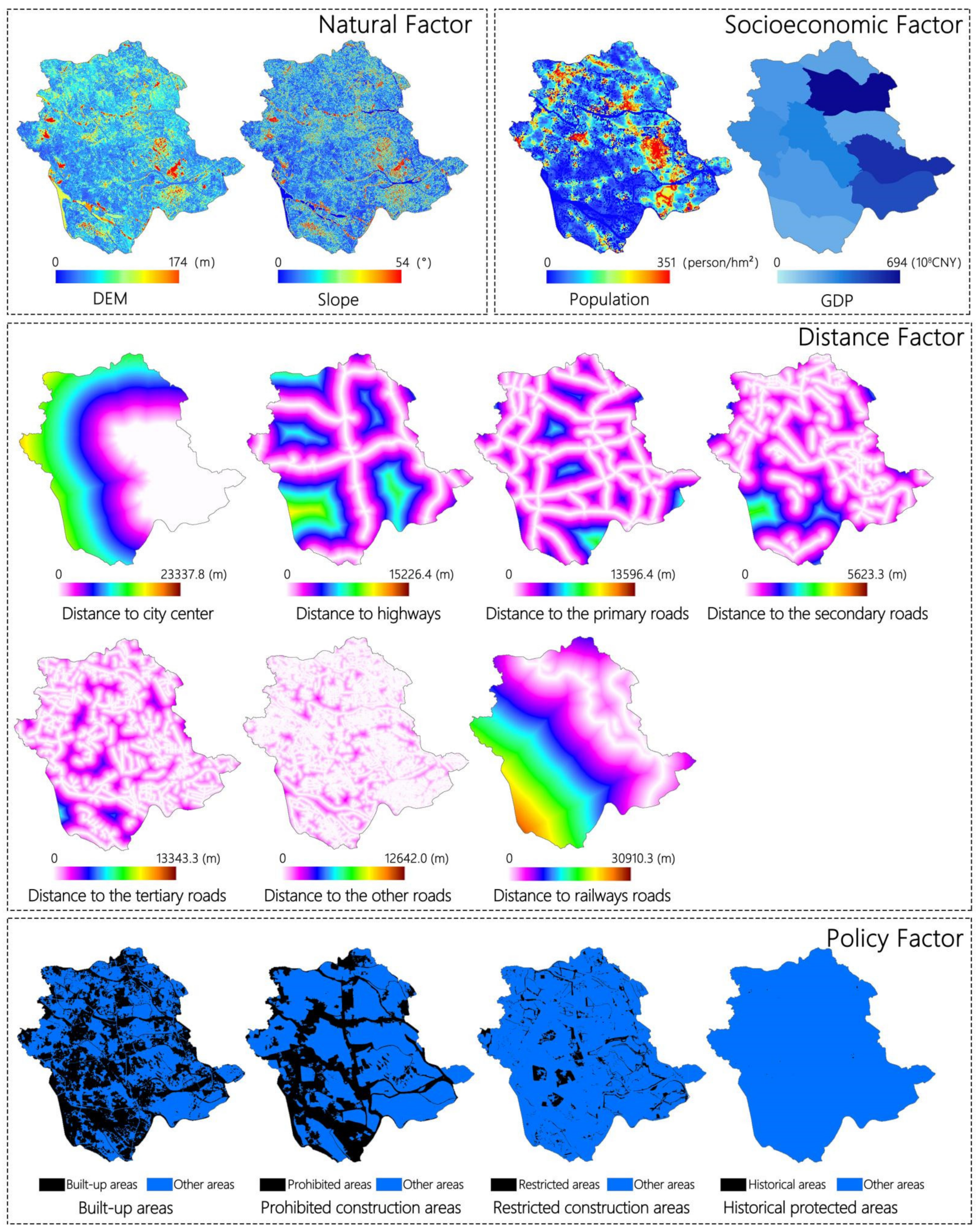
2.3.3. Multi-Criteria Evaluation

The conversion rule is central to the CA model. Multi-criteria evaluation (MCE) can transform various drivers into a transfer suitability atlas and then drive the transfer of cells, making the simulation more realistic. The accurate selection of the drivers of landscape pattern changes is key to the simulation. According to previous experience combined with regional development characteristics [63,64,65], 15 factors in four categories were selected as drivers of landscape pattern change (

Table 4. Driving factors of the suitability atlas for multi-criteria evaluation.

Driving Form	Type of Driving Factor	Data	Unit
Bottom-up	Natural	Slope	degree
		Altitude	m
	Socioeconomic	Population	pp/km2
		GDP	100 million
	Accessibility	Distance from the city center	m
		Distance from highways	m
		Distance from the primary roads	m
		Distance from the secondary roads	m
		Distance from the tertiary roads	m
		Distance from the other roads	m
		Distance from railways	m
Top-down	Policy	Prohibited construction areas	km2
		Restricted construction areas	km2
		Historical protected areas	km2
		Built-up areas	km2

). Bottom-up drivers include natural, socioeconomic, and accessibility factors, whereas top-down policy factors include extracting prohibited construction areas, restricted construction areas, historical protected areas, and built-up areas, according to the upper planning text.

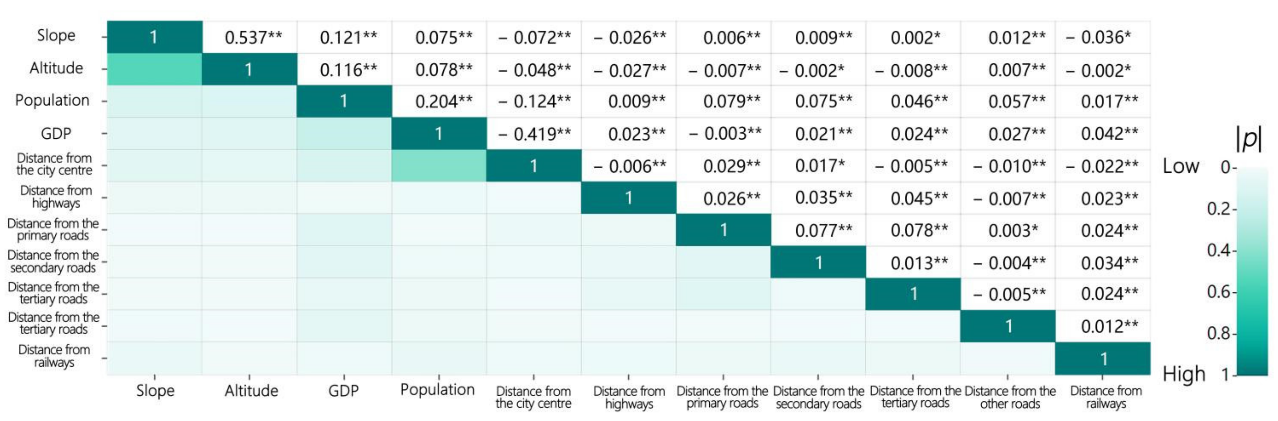
2.3.4. Evaluating Correlation

We computed Pearson’s correlation coefficients between the 11 top-down driving factors to evaluate their concordance. The Pearson’s correlation coefficient is calculated as follows [66]:

$$P=\frac{n({\displaystyle \sum xy})-({\displaystyle \sum x})({\displaystyle \sum y})}{\sqrt[]{\left[n{\displaystyle \sum x^2-{({\displaystyle \sum x^2})}^2}\right]\left[n{\displaystyle \sum y^2-{({\displaystyle \sum y})}^2}\right]}}$$

(4)

where P is the Pearson’s correlation coefficient between x and y, n is the number of pairs of variables, ∑xy is the sum of the products of the paired variables, ∑x is the sum of x, ∑y is the sum of y, ∑x² is the sum of x-squared, and ∑y² is the sum of y-squared. The Pearson’s correlation coefficients range from −1 to 1. A value of −1 indicates a strong negative relationship, 0 indicates no relationship, and 1 indicates a strong positive relationship.

2.3.5. Ecosystem Services Assessment

Based on the MA framework, Xie Gaodi et al. constructed a dynamic equivalent factor method for ESV assessment [67], which is widely used in large-scale ecosystem service assessments. Considering the regional differences and spatial heterogeneity of ESV, corrections were made in combination with the actual situation of Shunde District, based on the ESV scale [68] of Foshan city and Shunde District established by previous authors. Thus, the coefficient of ecosystem service value per unit area of Shunde District was obtained (

Table 5. Ecosystem service value coefficient per unit area in Shunde District (CNY/hm²).

Service Type	Service Index	Dike-Pond	Farmland	Forest	Water	Construction	Unused
Provisioning service	Food production	1532.53	4150.61	582.21	2460.31	37.56	88.69
	Raw material production	785.04	2610.56	1333.45	1371.01	112.68	177.37
	Water supply	8780.75	−4901.85	694.90	20,433.76	−3436.93	0.00
Regulating service	Gas regulation	1901.89	3343.02	4413.54	5014.53	450.74	1901.89
	Climate regulation	4573.80	1746.64	13,203.06	11,062.02	375.62	4573.80
	Hydrological regulation	116,838.01	507.09	3737.42	17,184.64	1352.23	310.40
	Purify environment	6820.02	5615.53	6592.14	237,523.62	845.14	1152.92
Supporting service	Soil retention	2024.60	1953.23	5371.37	6085.06	525.86	753.83
	Nutrient cycling	211.60	582.21	413.18	469.53	37.56	0.00
	Biodiversity	3609.71	638.55	4883.07	19,569.83	488.30	1773.72
Cultural service	Aesthetic landscape	2452.80	281.72	2141.04	12,433.03	206.60	1064.23
Total		149,530.76	16,527.31	43,365.38	333,607.34	995.36	11,796.85

).

The dike-pond is a compound land-use type where fruit, mulberry, and sugarcane trees are often planted on the base surface. It is classified as garden land, while massive pond land is classified as a pit pond. A dike-pond ratio of 4:6 is common because it can provide both economic and ecological benefits. Therefore, the dike-pond ESV coefficient in this study was calculated by adding 40% of the garden and 60% of the pit pond ESV coefficient.

In order to analyze the impact of regional landscape type change on ESV, the ESV was divided into five levels based on the natural breakpoint method: low, relatively low, medium, relatively high, and high.

3. Results

3.1. Evaluation of the Correlation and Simulation Results

Pearson correlation coefficients were used to analyze the correlation between top-down driving factors; Figure 2 shows that each correlation between the 11 driving factors was significant, and therefore could be used for landscape pattern simulation. As shown in Figure 2, the correlation between slope and elevation was the greatest, while the correlation between slope and distance from tertiary roads was the lowest.

Using the 2010 landscape classification map of Shunde District as the initial year, the CA-Markov model was used to simulate land use in 2020 (Figure 3b). The multi-criteria evaluation suitability atlas (Figure 4) was also added into the MCE-CA-Markov model to simulate land use in 2020 (Figure 3c). The simulation accuracy was evaluated by comparing the simulation classification results with the landscape remote sensing interpretation classification results (Figure 3a). The Kappa index using the CA-Markov model was 0.7711, while the index of the MCE-CA-Markov model was 0.8032, indicating that the MCE-CA-Markov model was more accurate and feasible. The MCE suitability atlas is sensitive to changes in construction land because it considers social and economic factors (Figure 3(a(1),a(3),c(1),c(3))) but the transformation of built-up areas to other land use types is restricted because of the influence of policy factors, which makes the simulation results more realistic (Figure 3(a(2),c(2))).

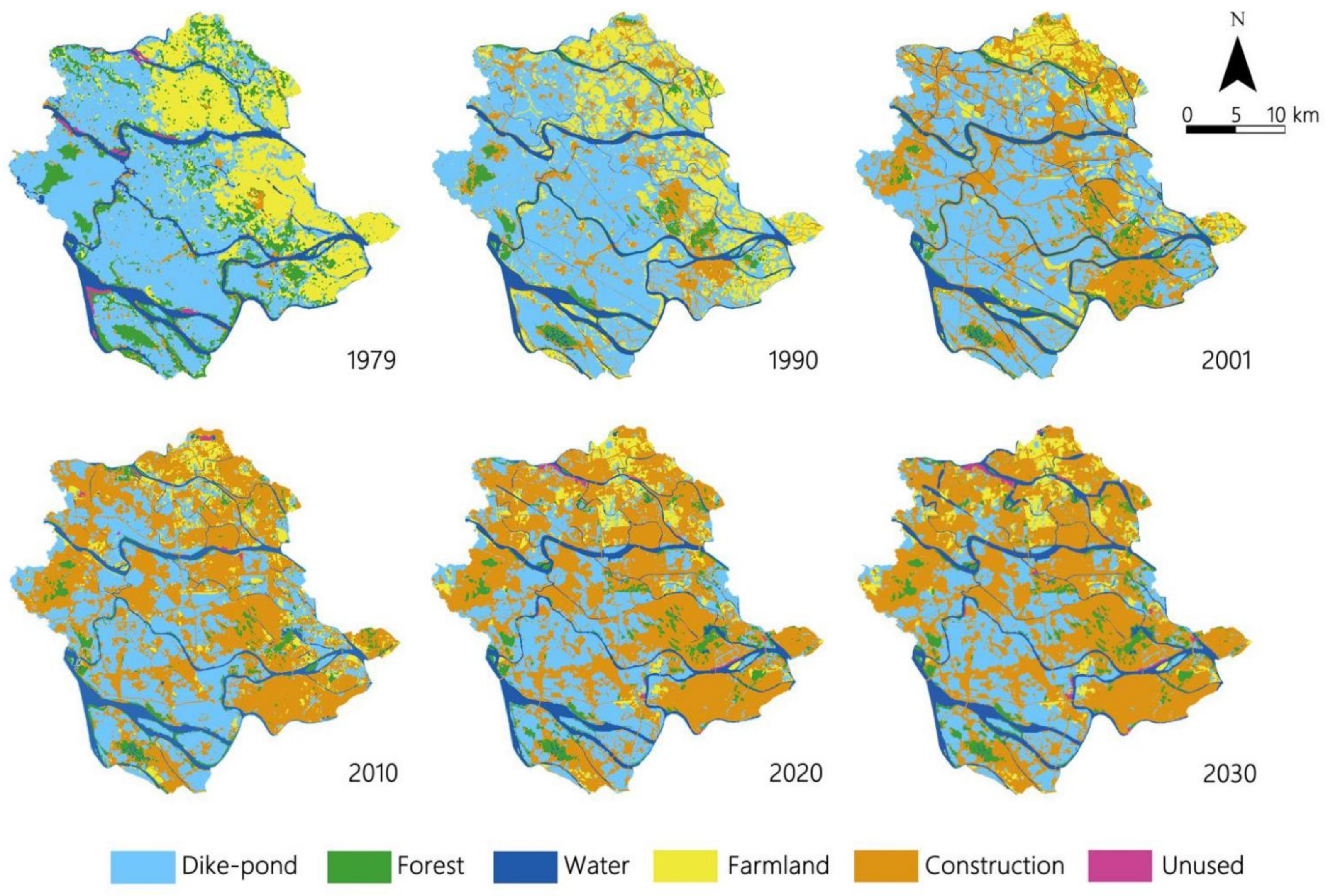
3.2. Spatio-Temporal Dynamics and Evolution of LUCC from 1979 to 2030

3.2.1. LUCC Process

From 1979 to 2030, the dike-pond area first increased then decreased (

Table 6. Area and proportion of dike-ponds in the study area from 1979 to 2030.

Year	Foundation Pond Area (km2)	Dike-Pond Area (%)
1979	368.79	45.61
1990	406.66	50.27
2001	362.39	44.80
2010	255.12	31.57
2020	219.47	27.16
2030	198.85	24.61

). Before 1990, the dike-pond area increased and spread from the central and western areas to Chen Cun Town and Bei Jiao Town in the north, and Lun Jiao and Da Liang streets in the east. From 2001 to 2020, the dike-pond area decreased rapidly, and construction land became the dominant land use type. The dike-pond in the north, east, and west shrank dramatically, leaving only sporadic distribution. By 2020, the dike-pond area was mainly distributed throughout central Le Liu Street, Xing Tan Town, and Jun An Town in the south. The simulated landscape pattern and data for 2030 show that the dike-pond area will continue to decrease in the future, but at a slightly slower rate (Figure 5).

3.2.2. Matrix Analysis of Land Use Change

To determine the specific transformation direction and quantity of dike-ponds, a Markov chain was used to calculate the area transfer matrix of the dike-ponds in the study area from 1979 to 2030 (

Table 7. Area transfer matrix of dike-pond land in the study area from 1979 to 2030.

Transfer Type	Transfer Direction	Land Area Transformed within Each Time Range (km2)
		1979–1990	1990–2001	2001–2010	2010–2020	2020–2030	Sum		Mean
Transformation from dike-pond	Dike-pond→Farmland	−16.3	−16.6	−21.8	−15.0	−6.3	−76.0	−466.4	−3.33 /year
	Dike-pond→Construction	−44.7	−97.6	−126.1	−50.3	−11.0	−329.7
	Dike-pond→Forest	−6.7	−7.1	−9.6	−6.9	−6.5	−36.8
	Dike-pond→Water	−6.3	−5.8	−4.6	-3.4	−1.0	−21.1
	Dike-pond→Unused	−0.6	−0.8	−0.7	−0.5	−0.2	−2.8
Transformation into dike-pond	Farmland→Dike-pond	31.9	67.6	11.2	4.7	0.3	115.7	296.5
	Construction→Dike-pond	9.1	19.3	19.9	25.1	3.6	77.0
	Forest→Dike-pond	62.5	6.4	4.0	5.1	1.2	79.2
	Water→Dike-pond	7.7	5.6	4.5	4.1	0.5	22.4
	Unused→Dike-pond	0.6	1.1	0.3	0.2	0.0	2.2
Sum		37.2	−27.9	−122.9	−36.9	−19.4	−169.9

). In this period, the most obvious conversion was from dike-pond to construction land. From 1979 to 2010, this conversion increased continuously and from 2001 to 2010, the area that had changed from dike-pond to construction land was the largest but this then decreased because Shunde District is at the forefront of the Chinese economic reform and its industry (including tertiary industry) developed vigorously from 1979 to 2001. Part of the dike-pond was used for urban construction and industrial development. From 2001 to 2010, with the intensification of competition among cities, Shunde began the strategic transformation of urbanization, with the rapid expansion of construction land, which was mainly transferred from dike-pond areas. After 2010, The Promulgate Plan for The Protection and Development of Pearl River Delta Dike-Pond Agricultural System in Foshan, Guangdong promoted ecological civilization in Foshan, and the area of dike-ponds converted into construction land decreased significantly.

Most land that was transformed into dike-pond from 1979 to 2030 began as farmland. From 1979 to 1990, a large area of forest land was transformed into dike-pond as agriculture in the area in 1979–2001 shifted from planting to breeding, and mulberry- and sugarcane-based dike-ponds developed vigorously and became pillars of the regional economy. Therefore, large areas of farmland and forest have been transformed into dike-pond in order to develop dike-pond agriculture. According to the simulation data, from 2020 to 2030, the amount of land transformed from dike-pond will slightly decrease, but the main conversion would remain dike-pond to construction, indicating that efforts to protect dike-ponds need to be increased. Overall, from 1979 to 2030, the total area of dike-pond is predicted to decrease by 169.9 km², and 3.33 km² of dike-pond will be converted to other land types each year.

3.3. Spatiotemporal Evolution Analysis of Landscape Patterns

3.3.1. Analysis of Spatial Metrics at the Class Scale

From 1979 to 1990, the LPI and AWMPFD of dike-pond areas showed an upward trend, while MPS significantly decreased, indicating that dike-pond was the most dominant landscape type. The degree of fragmentation increased sharply, indicating that, in addition to the original dike-ponds, a large number of new dike-ponds were artificially developed (Figure 6). Combined with Figure 4 and Table 5, farmland adjacent to dike-ponds was transformed into dike-ponds, particularly in Chen Cun Town and Bei Jiao Town in the northeast. From 1990 to 2001, the LPI, AWMPFD, and COHESION of dike-ponds decreased rapidly and the MPS increased significantly, while the LPI and MPS of construction land continued to rise. The construction land surpassed dike-ponds and became the largest dominant landscape type, indicating that the sprawl growth of buildings broke up the original blocks of dike-ponds, resulting in a sharp rise in fragmentation and a decline in COHESION. AWMPFD decreased significantly because during this period some natural dike-ponds were artificially altered to form a regular shape to improve their production efficiency for aquaculture.

From 2001 to 2010, the ecological value of dike-pond areas began to attract attention, and their LPI, AWMPFD, and COHESION increased, while the MPS decreased. At this stage, the dominance and COHESION of the dike-pond areas increased, and the impact of human activities decreased. From 2010 to 2020, the four indices decreased slightly, and the degrees of dominance, aggregation, and fragmentation decreased. In the simulation for 2020–2030, the four indexes did not change significantly, and the dominance of construction land decreased, showing that slower-paced urbanization and regional development tends to be stable.

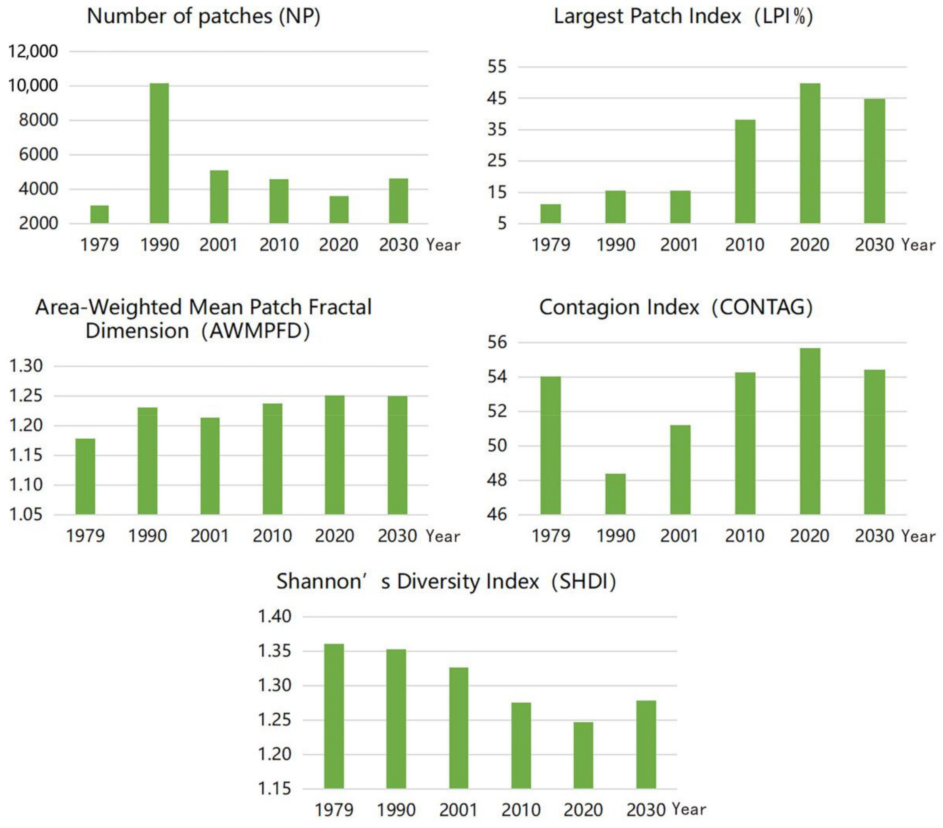
3.3.2. Analysis of the Spatial Metrics at the Landscape Scale

As shown in Figure 7, landscape fragmentation in Shunde increased from 1979 to 1990 and landscape connectivity and fragmentation decreased, connectivity increased, and spatial heterogeneity decreased. The LPI increased from 1979 to 2020, while the SHDI decreased, indicating that the area of the dominant landscape increased, and each type presented an unbalanced trend distribution within the landscape. The AWMPFD showed an overall increasing trend from 1979 to 2020, i.e., the complexity of the landscape shape increased. Combined with the decrease in NP from 1990 to 2020, this demonstrates that landscape fragmentation was the main cause of landscape pattern change from 1979 to 1990, and landscape shape complexity was the main cause of landscape pattern change from 1990 to 2020. The landscape index calculated by combining the simulation results shows that NP and SHDI increased while LPI, AWMPFD, and CONTAG decreased from 2020 to 2030, indicating that the dominance degree of the dominant landscape in the region decreased, while the overall landscape richness improved. Anthropogenic disturbance still increased, leading to a decrease in the degree of fragmentation and aggregation of the region. However, compared to the previous stage, the rate of decrease was significantly slower.

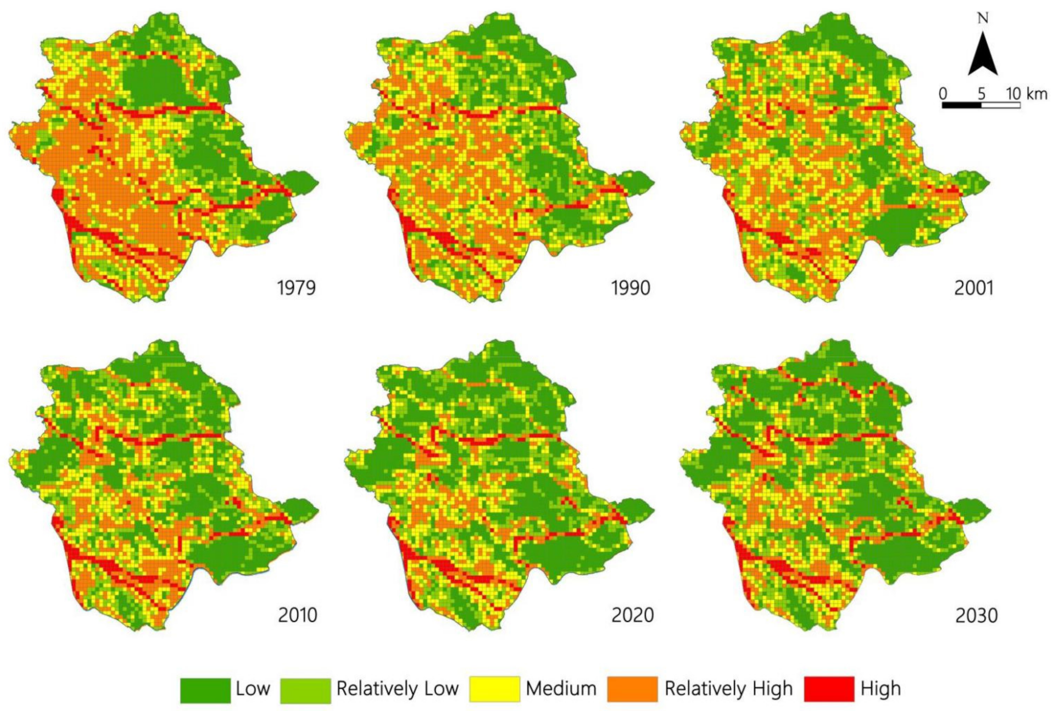
3.4. Spatio-Temporal Evolution of ESV

As shown in Figure 8, the dike-pond has always been the landscape type with the highest ESV contribution, and the change trend of the dike-pond ESV is consistent with that of the overall ESV. This indicates that the dike-pond is the main landscape type that maintains ecological balance in the study area. From 1979 to 2020, the ESV in Shunde showed a downward trend, with the largest decline from 2001 to 2010. Figure 9 shows the spatial evolution of ESV in the study area from 1979 to 2030. In 1979, the spatial distribution of ESV in Shunde District was clearly differentiated, showing a spatial pattern characteristic of high ESV in the south and west, and low ESV in the north and east. From 1979 to 2001, the ESV of the central and marginal areas in the south and west began to decline, and the high ESV area spread eastward, which was due to the development of construction land in the west and the increase in dike-pond in the east. In the following two decades, dike-pond agriculture was replaced by modern agriculture, and the ESV of the study area decreased significantly. The simulation results show that from 2020 to 2030, the ESV in Shunde declined on the whole, but at a slower rate than previous years. Simultaneously, the ESV along the river in the northern area will improve significantly, but the ESV of the dike-pond will continue to decrease. This means that dike-pond protection must be strengthened.

4. Discussion

4.1. Optimization of the MCE Module

In recent years, Foshan City has issued several plans and policies for dike-pond protection. When setting the driving factors in the MCE module in this study, in addition to the common bottom-top natural, socioeconomic, and accessibility factors [69,70], top-down policy factors were also considered; this was implemented to make the simulation results more realistic. In addition, the simulation results can reverse verify the completion of upper position planning in the study area. Previous studies mostly calculated multiple levels of roads uniformly when considering distance from roads as a driving factor [24,71]. However, different road levels often have different driving abilities for landscape pattern changes. Therefore, this study divided roads into highways, primary roads, secondary roads, tertiary roads, other roads, and railways. Different parameters were set for each type of road to make the model transfer rules more realistic and effective.

4.2. Dike-Pond Development Model Based on ESV and Landscape Patterns

The dike-pond is an important part of the rural land space in Shunde and the Pearl River Delta. Combined with the current spatial metrics and ESV, the corresponding development mode was proposed according to the different characteristics of the dike-pond (Figure 10):

(1)

Dike-pond ecological zone. The areas of the dike-pond with high ESV are usually distributed along the river, and the areas with high ESV are the dike-pond groups with a low landscape fragmentation degree, high degree of agglomeration, and obvious dominance degree. These areas can contribute high ecological value alone or in combination with the surrounding water system and they play a key role in maintaining regional ecological stability. Therefore, this zone should not be disturbed by human beings, and ecological protection red lines should be set to allow them to grow freely and restore their ecology.

(2)

Dike-pond development zone. The median ESV area of the dike-pond was generally distributed around the higher value area close to the construction land. These dike-ponds have a medium degree of fragmentation and general connectivity. With little artificial transformation, traditional dike-ponds can be transformed into high-standard modern dike-ponds, and the economic benefits of agricultural production can be maximized through high-tech means.

(3)

Dike-pond living zone. Areas with low ESV values were distributed outside the middle planting area or scattered within construction land, with a high degree of fragmentation and complex patch shape. These scattered dike-ponds can be repaired using aquatic plant communities and gentle slopes to build ecological parks or wetland parks with the added values of recreation, science popularization, and education.

Figure 10. Spatial distribution of dike-pond ESVs in 2020.

Figure 10. Spatial distribution of dike-pond ESVs in 2020.

4.3. Research Limitations and Future Development Direction

One limitation is that SVM-supervised classification is based on the spectral characteristics of ground objects. Due to the image resolution, narrow base surface of the ponds, and the similar spectral characteristics of the pond surface and water body, the classification results will not differentiate between ponds and water bodies, so it is necessary to manually adjust the classification results. In this study, nine landscape indices were used to analyze the spatial metrics of dike-ponds, according to previous studies [72]. However, whether these nine indices can fully grasp the characteristics of spatial metric changes within this particular region needs to be verified.

In the past 10 years, the research on LULC driving mechanism has been gradually deepened. At present, the methods of multiple linear regression, geographically weighted regression (GWR), GeoDetector analysis, and Cramer’s V analysis are widely used to quantitatively determine the explanatory power of factors on LULC [73,74,75]. In this paper, Pearson correlation coefficients were used to analyze the correlation between top-down driving factors. However, the current analysis cannot determine which factor is majorly controlling the LULC change statistically. In our future research, we will work out an appropriate method to quantitatively analyze the correlation between spatial metrics and driving factors and clarify the key controlling factors for the LULC change.

Based on the ESV coefficient of Foshan City and Shunde District provided by previous research, this study did not consider the influence of time or specific farmed animals; each year, the variable pond aquaculture fish market prices are responsible for the food production index, which means the ecological deterioration of ponds leads to differences in the food diversity index, and so on. This study analyzed the response of ESV to spatial metrics from the perspective of spatial pattern evolution. In the future, the response degree should be quantitatively analyzed through spatial autocorrelation analysis, clustering, and outlier analysis in order to guide the optimization of regional landscapes and urban planning.

5. Conclusions

Based on remote sensing images and the MCE-CA-Markov model combined with a transfer matrix and spatial metrics, the spatiotemporal evolution of dike-ponds in Shunde was simulated, and its landscape patterns were studied. Research shows that dike-ponds in Shunde have always been predominant, first increasing then decreasing in area. The aim of the study was to understand the spatial and temporal evolution process of dike-pond landscape patterns and ESV, to predict the dike-pond landscape in 2030, and to provide references for future development of the city. The main findings can be summarized as follows:

(1)

By integrating top-down and bottom-up driving factors, and setting different parameters according to different road grades, the MCE-CA-Markov model is feasible in land use simulation with high precision and good simulation effect.

(2)

In Shunde, from 1979 to 2020, in terms of LUCC, dike-pond, arable land, and forest land were transformed into construction land. In the simulation, dike-pond area continued to decrease until 2030, and the proportion of dike-pond converted into construction land was the largest, but the rate of decline slowed slightly.

(3)

The development of urbanization will lead to the change in dominant landscape and the increase in fragmentation of the dike-pond landscape. The change in landscape patterns in the study area can be divided into three stages at the class scale. From 1979 to 1990, dike-pond was the dominant landscape type in Shunde, with obvious dominance but a high degree of fragmentation. From 1990 to 2001, with the acceleration of urbanization, the dominance degree of the dike-pond and the degree of agglomeration decreased, but the degree of fragmentation and shape complexity also decreased. From 2001 to 2020, due to rapid urbanization, the dominance degree of dike-ponds decreased continuously, and the fragmentation degree and shape complexity increased. At the landscape scale, the overall landscape exhibited an unbalanced trend. Before 1990, landscape fragmentation dominated landscape pattern changes. After 1990, the change in landscape patterns was reflected in the complexity of the landscape patch shape. From 2020 to 2030, the decline rate of the fragmentation degree and degree of aggregation slowed significantly, and the overall landscape richness increased.

(4)

For agricultural countries and regions, agroecosystem accounts for a large proportion in regional ecosystem services. In this study, for example, dike-pond contributes the most to ESV and is the main landscape type that maintains ecological balance in Shunde. Over the past four decades, the ESV in Shunde has decreased significantly, with the largest decline from 2001 to 2010. Therefore, dike-pond protection should be further strengthened in rural planning and regional development should improve the regional ecosystem service value and maintain the stability of rural landscapes in the future.

References

1. Gu, C.; Hu, L.; Cook, I.G. China’s urbanization in 1949–2015: Processes and driving forces. Chin. Geogr. Sci. 2017, 27, 847–859. [Google Scholar] [CrossRef]
2. Long, H.; Liu, Y.; Hou, X.; Li, T.; Li, Y. Effects of land use transitions due to rapid urbanization on ecosystem services: Implications for urban planning in the new developing area of China. Habitat Int. 2014, 44, 536–544. [Google Scholar] [CrossRef]
3. Zhong, G.F. Mulberry Fish Pond in The Pearl River Delta:an artificial ecosystem with interaction between land and water. J. Geogr. 1980, 35, 200–208. [Google Scholar]
4. Lo, C.P. Environmental impact on the development of agricultural technology in China: The case of the dike-pond (‘jitang’) system of integrated agriculture-aquaculture in the Zhujiang Delta of China. Agric. Ecosyst. Environ. 1996, 60, 183–195. [Google Scholar] [CrossRef]
5. Xi, Q.; Guo, W. Study on vernacular landscape in Sangyuanwei area from the perspective of landscape architectur. Chin. Archit. Cult. 2015, 12, 169–171. [Google Scholar]
6. Guo, S. The value and Utilization of Mulberry-Dike-Fish-Pond in the Pearl River Delta Perspective of the Agricultural Heritage. Trop. Geogr. 2010, 30, 452–458. [Google Scholar]
7. Huang, S.R. Yue zhong can sang chu yan and “Sang Ji Yu Tang” in the delta of the Pearl River. China Hist. Mater. Sci. Technol. 1990, 11, 83–87. [Google Scholar]
8. Zhong, G. Characteristics and practical significance of dike-pond system. Sci. Geogr. Sin. 1988, 12, 12–17. [Google Scholar]
9. Korn, M. The dike-pond concept: Sustainable agriculture and nutrient recycling in China. Ambio Swed. 1996, 25, 6–13. [Google Scholar]
10. Zhong, G.F. The mulberry dike-fish pond complex: A Chinese ecosystem of land-water interaction on the Pearl River Delta. Hum. Ecol. 1982, 10, 191–202. [Google Scholar]
11. Hu, W.W.; Wang, G.X.; Deng, W. Advance in research of the relationship between landscape patterns and ecological processes. Prog. Geogr. 2008, 27, 18–24. [Google Scholar]
12. Nie, C.R.; Luo, S.M.; Zhang, J.E. Degradation and ecological restoration of dike-pond system under modern intensive agriculture. Acta Ecol. Sin. 2003, 23, 1851–1860. [Google Scholar]
13. Guo, C.X.; Xu, S.J. Research progress and new perspective of Dike-pond system in China. Wetl. Sci. 2011, 9, 75–81. [Google Scholar]
14. Jiao, M.; Hu, M.M.; Xia, B.C. Spatiotemporal dynamic simulation of land-use and landscape pattern in the Pearl River Delta, China. Sustain. Cities Soc. 2019, 49, 101581. [Google Scholar] [CrossRef]
15. Hu, M.M.; Li, Z.T.; Wang, Y.F.; Jiao, M.Y.; Li, M.; Xia, B.C. Spatio-temporal changes in ecosystem service value in response to land-use/cover changes in the Pearl River Delta. Resour. Conserv. Recycl. 2019, 149, 106–114. [Google Scholar] [CrossRef]
16. Ding, J.H.; Wen, Y.M.; Shu, Q. Current situation, problems and countermeasures of sustainable development of dike-pond system. Chongq. Environ. Sci. 2001, 5, 12–14. [Google Scholar]
17. Nie, C.R.; Li, H.T. Dike-pond system: Current situation, problems and prospects. J. Foshan Univ. Sci. Technol. 2001, 1, 49–53. [Google Scholar]
18. Yang, H.F.; Zhong, X.N.; Deng, S.Q.; Nie, S.N.; Godron, M. Impact of LUCC on landscape pattern in the Yangtze River Basin during 2001–2019. Ecol. Inf. 2022, 69, 101631. [Google Scholar] [CrossRef]
19. Abdullah, S.A.; Nakagoshi, N. Changes in landscape spatial pattern in the highly developing state of Selangor, peninsular Malaysia. Landsc. Urban Plan. 2006, 77, 263–275. [Google Scholar] [CrossRef]
20. Soto, M.R.; Clavé, S.A. Second homes and urban landscape patterns in Mediterranean coastal tourism destinations. Land Use Policy 2017, 68, 117–132. [Google Scholar] [CrossRef]
21. Aguilera, F.; Valenzuela, L.M.; Botequilha-Leitão, A. Landscape metrics in the analysis of urban land use patterns: A case study in a Spanish metropolitan area. Landsc. Urban Plan. 2011, 99, 226–238. [Google Scholar] [CrossRef]
22. Shukla, A.; Jain, K. Analyzing the impact of changing landscape pattern and dynamics on land surface temperature in Lucknow city, India. Urban For. Urban Green. 2020, 58, 126877. [Google Scholar] [CrossRef]
23. Ramachandra, T.V.; Aitha, B.H.; Sanna, D.D. Insights to urban dynamics through landscape spatial pattern analysis. Int. J. Appl. Earth Obs. Geoinf. 2012, 18, 329–343. [Google Scholar]
24. Fu, F.; Deng, S.; Wu, D.; Liu, W.W.; Bai, Z.H. Research on the spatiotemporal evolution of land use landscape pattern in a county area based on CA-Markov model. Sustain. Cities Soc. 2022, 80, 103760. [Google Scholar] [CrossRef]
25. Yohannes, H.; Soromessa, T.; Argaw, M.; Dewan, A. Impact of landscape pattern changes on hydrological ecosystem services in the Beressa watershed of the Blue Nile Basin in Ethiopia. Sci. Total Environ. 2021, 793, 148559. [Google Scholar] [CrossRef]
26. Su, W.Z.; Gu, C.L.; Yang, G.S.; Chen, S.; Zhen, F. Measuring the impact of urban sprawl on natural landscape pattern of the Western Taihu Lake watershed, China. Landsc. Urban Plan. 2010, 95, 61–67. [Google Scholar] [CrossRef]
27. Ripple, W.J.; Bradshaw, G.A.; Spies, T.A. Measuring forest landscape patterns in the cascade range of Oregon, USA. Biol. Conserv. 1991, 57, 73–88. [Google Scholar] [CrossRef]
28. Lin, W.P.; Cen, J.W.; Xu, D.; Du, S.Q.; Gao, J. Wetland landscape pattern changes over a period of rapid development (1985–2015) in the ZhouShan Islands of Zhejiang province, China. Estuar. Coast. Shelf Sci. 2018, 213, 148–159. [Google Scholar] [CrossRef]
29. Bai, J.H.; Ouyang, H.; Cui, B.S.; Wang, Q.G.; Chen, H. Changes in landscape pattern of alpine wetlands on the Zoige Plateau in the past four decades. Acta Ecol. Sin. 2008, 28, 2245–2252. [Google Scholar]
30. Ye, C.S. Change characteristics and spatial types of dike-pond in pearl River Delta. J. China Inst. Technol. 2013, 36, 315–322. [Google Scholar]
31. Liu, K.; Wang, S.G.; Xie, L. Spatial pattern evolution of Dike-pond system in Foshan City. Trop. Geogr. 2008, 28, 513–517. [Google Scholar]
32. Han, X.L.; Yu, K.J.; Li, D.H. Construction of dike-urban landscape security pattern: A case study of Magang District, Shunde District, Foshan City. Reg. Res. Dev. 2008, 27, 107–110. [Google Scholar]
33. Pontius, R.G., Jr.; Huffaker, D.; Denman, K. Useful techniques of validation for spatially explicit land-change models. Ecol. Model. 2004, 179, 445–461. [Google Scholar] [CrossRef]
34. Zhao, X.; Yi, P.; Xia, J. Temporal and spatial analysis of the ecosystem service values in the Three Gorges Reservoir area of China based on land use change. Environ. Sci. Pollut. Res. 2021, 21, 17827. [Google Scholar] [CrossRef] [PubMed]
35. Hu, B.; Zhang, H.; Li, Y. Spatiotemporal variation analysis of driving forces of urban land spatial expansion using logistic regression: A case study of port towns in Taicang City, China. Habitat Int. 2014, 43, 181–190. [Google Scholar]
36. Esgalhado, C.; Guimares, H.; Debolini, M. A holistic approach to land system dynamics–The Monfurado case in Alentejo, Portugal. Land Use Policy 2020, 95, 104607. [Google Scholar] [CrossRef]
37. Ibarra-Bonilla, J.S.; Villarreal-Guerrero, F.; Prieto-Amparán, J.A.; Santellano-Estrada, E.; Pinedo-Alvarez, A. Characterizing the impact of Land-Use/Land-Cover changes on a Temperate Forest using the Markov model. Egypt. J. Remote Sens. Space Sci. 2021, 24, 1013–1022. [Google Scholar] [CrossRef]
38. Xun, L.; Qga, B.; Kcc, C. Mixed-cell cellular automata: A new approach for simulating the spatio-temporal dynamics of mixed land use structures. Landsc. Urban Plan. 2021, 205, 103960. [Google Scholar]
39. Liu, X.; Xun, L.; Xia, L. A future land use simulation model (FLUS) for simulating multiple land use scenarios by coupling human and natural effects. Landsc. Urban Plan. 2017, 168, 94–116. [Google Scholar] [CrossRef]
40. Wang, Y.A.; Shen, J.B.; Yan, W.C. Backcasting approach with multi-scenario simulation for assessing effects of land use policy using GeoSOS-FLUS software. MethodsX 2019, 6, 1384–1397. [Google Scholar] [CrossRef]
41. Yirsaw, E.; Wu, W.; Shi, X.; Temesgen, H.; Bekele, B. Land use/land cover change modeling and the prediction of subsequent changes in ecosystem service values in a coastal area of China, the Su-Xi-Chang Region. Sustainability 2017, 9, 1204. [Google Scholar] [CrossRef]
42. Gashaw, T.; Tulu, T.; Argaw, M.; Worqlul, A.W.; Tolessa, T.; Kindu, M. Estimating the impacts of land use/land cover changes on Ecosystem Service Values: The case of the Andassa watershed in the Upper Blue Nile basin of Ethiopia. Ecosyst. Serv. 2018, 31, 219–228. [Google Scholar] [CrossRef]
43. Wang, Q.; Wang, H.; Chang, R. Dynamic simulation patterns and spatiotemporal analysis of land-use/land-cover changes in the Wuhan metropolitan area, China. Ecol. Model. 2022, 464, 109850. [Google Scholar] [CrossRef]
44. Arasteh, R.; Abbaspour, R.A.; Salmanmahiny, A. A modeling approach to path dependent and non-path dependent urban allocation in a rapidly growing region. Sustain. Cities Soc. 2018, 44, 378–394. [Google Scholar] [CrossRef]
45. Hao, W.; Yha, B.; Yla, B. Simulation and spatiotemporal evolution analysis of biocapacity in Xilingol based on CA-Markov land simulation-ScienceDirect. Environ. Sustain. Indic. 2021, 11, 100136. [Google Scholar]
46. Drobyshev, I.; Ryzhkova, N.; Niklasson, M. Marginal imprint of human land use upon fire history in a mire-dominated boreal landscape of the Veps Highland, North-West Russia. For. Ecol. Manag. 2022, 507, 120007. [Google Scholar] [CrossRef]
47. Loomes, R.; O’Neill, K. Nature’s services: Societal dependence on natural ecosystems. Pac. Conserv. Biol. 1997, 6, 220–221. [Google Scholar] [CrossRef]
48. Mla, B.; Yja, B.; Jza, B. Revegetation projects significantly improved ecosystem service values in the agro-pastoral ecotone of northern China in recent 20 years. Sci. Total Environ. 2021, 788, 147756. [Google Scholar]
49. Jing, L.; Jiaxin, L.; Yue, W. Quantitative evaluation of ecological cumulative effect in mining area using a pixel-based time series model of ecosystem service value. Ecol. Indic. 2021, 120, 106873. [Google Scholar]
50. Zheng, D.; Wang, Y.; Hao, S. Spatial-temporal variation and tradeoffs/synergies analysis on multiple ecosystem services: A case study in the Three-River Headwaters region of China-ScienceDirect. Ecol. Indic. 2020, 116, 106494. [Google Scholar] [CrossRef]
51. Lin, Y.P.; Chen, C.J.; Lien, W.Y.; Chang, W.H.; Petway, J.R.; Chiang, L.C. Landscape conservation planning to sustain ecosystem services under climate change. Sustainability 2019, 11, 1393. [Google Scholar] [CrossRef]
52. Costanza, R.; d’Arge, R.; Groot, R.D. The value of the world’s ecosystem services and natural capital. Nature 1997, 387, 253–260. [Google Scholar] [CrossRef]
53. Guo, P.F.; Zhang, F.F.; Wang, H.Y. The response of ecosystem service value to land use change in the middle and lower Yellow River: A case study of the Henan section. Ecol. Indic. 2021, 140, 109019. [Google Scholar] [CrossRef]
54. Li, F.; Liu, K.; Tang, H.; Liu, L.; Liu, H. Analyzing trends of dike-ponds between 1978 and 2016 using multi-source remote sensing images in Shunde district of south China. Sustainability 2018, 10, 3504. [Google Scholar] [CrossRef]
55. Wei, Y.; Zhang, Z. Assessing the fragmentation of construction land in urban areas: An index method and case study in Shunde, China. Land Use Policy 2012, 29, 417–428. [Google Scholar] [CrossRef]
56. Song, C.; Sun, C.; Xu, J.; Fan, F. Establishing coordinated development index of urbanization based on multi-source data: A case study of Guangdong-Hong Kong-Macao Greater Bay Area, China. Ecol. Indic. 2022, 140, 109030. [Google Scholar] [CrossRef]
57. Das, D.N.; Chakraborti, S.; Saha, G.; Banerjee, A.; Singh, D. Analysing the dynamic relationship of land surface temperature and landuse pattern: A city level analysis of two climatic regions in India. City Environ. Indic. 2020, 8, 100046. [Google Scholar] [CrossRef]
58. McGarigal, K.; Marks, B.J. FRAGSTATS: Spatial Pattern Analysis Program for Quantifying Landscape Structure; USDA Forest Service-General Technical Report PNW; US Forest Service Pacific Northwest Research Station: Corvallis, OR, USA, 1995; Volume 351.
59. Okwuashi, O.; Ndehedehe, C.E. Integrating machine learning with Markov chain and cellular automata models for modelling urban land use change. Remote Sens. Appl. Soc. Environ. 2020, 21, 100461. [Google Scholar] [CrossRef]
60. Deng, J.S.; Ke, W.; Yang, H. Spatio-temporal dynamics and evolution of land use change and landscape pattern in response to rapid urbanization. Landsc. Urban Plan. 2009, 92, 187–198. [Google Scholar] [CrossRef]
61. Ghalehteimouri, K.J.; Shamsoddini, A.; Mousavi, M.N.; Ros, F.B.C.; Khedmatzadeh, A. Predicting spatial and decadal of land use and land cover change using integrated cellular automata Markov chain model based scenarios (2019–2049) Zarriné-Rūd River Basin in Iran. Environ. Chall. 2020, 21, 100461. [Google Scholar] [CrossRef]
62. Girma, R.; Fürst, C.; Moges, A. Land use land cover change modeling by integrating artificial neural network with cellular Automata-Markov chain model in Gidabo river basin, main Ethiopian rift. Environ. Chall. 2021, 6, 100419. [Google Scholar] [CrossRef]
63. Fu, X.; Wang, X.H.; Yang, Y.J. Deriving suitability factors for CA-Markov land use simulation model based on local historical data. J. Environ. Manag. 2017, 206, 10. [Google Scholar] [CrossRef]
64. Zzab, C.; Bha, B.; Wjd, E. Identification and scenario prediction of degree of wetland damage in Guangxi based on the CA-Markov model. Ecol. Indic. 2021, 127, 107764. [Google Scholar]
65. Zhang, Y.; Chang, X.; Liu, Y.; Lu, Y.; Wang, Y.; Liu, Y. Urban expansion simulation under constraint of multiple ecosystem services (MESs) based on cellular automata (CA)-Markov model: Scenario analysis and policy implications. Land Use Policy 2021, 108, 105667. [Google Scholar] [CrossRef]
66. Wu, H.; Fang, S.M.; Yang, Y.Y.; Cheng, J. Changes in habitat quality of nature reserves in depopulating areas due to anthropogenic pressure: Evidence from Northeast China, 2000–2018. Ecol. Indic. 2022, 138, 108844. [Google Scholar] [CrossRef]
67. Qiu, J.; Huang, T.; Yu, D. Evaluation and optimization of ecosystem services under different land use scenarios in a semiarid landscape mosaic. Ecol. Indic. 2022, 135, 108516. [Google Scholar] [CrossRef]
68. Li, L.; Wu, D.F.; Wang, F. Ecosystem service value prediction and tradeoff in rapidly urbanizing regions of China: A case study of Foshan City. Acta Ecol. Sin. 2020, 40, 14. [Google Scholar]
69. Yang, D.; Zhang, P.Y.; Jiang, L.; Zhang, Y.; Liu, Z.Y.; Rong, T.Q. Spatial change and scale dependence of built-up land expansion and landscape pattern evolution—Case study of affected area of the lower Yellow River. Ecol. Indic. 2022, 141, 109123. [Google Scholar] [CrossRef]
70. Geng, J.; Shen, S.; Cheng, C.; Dai, K. A hybrid spatiotemporal convolution-based cellular automata model (ST-CA) for land-use/cover change simulation. Int. J. Appl. Earth Obs. Geoinf. 2022, 110, 102789. [Google Scholar] [CrossRef]
71. Zhang, F.; Chen, Y.; Wang, W.W.; Jim, C.Y.; Zhang, Z.M. Impact of land-use/land-cover and landscape pattern on seasonal in-stream water quality in small watersheds. J. Clean. Prod. 2022, 357, 131907. [Google Scholar] [CrossRef]
72. Yl, A.; Jhab, C.; Jja, C. Responses of flood peaks to land use and landscape patterns under extreme rainstorms in small catchments-A case study of the rainstorm of Typhoon Lekima in Shandong, China. Int. Soil Water Conserv. Res. 2022, 10, 228–239. [Google Scholar]
73. Wang, Q.; Wang, H.J. Spatiotemporal dynamics and evolution relationships between land-use/land cover change and landscape pattern in response to rapid urban sprawl process: A case study in Wuhan, China. Ecol. Eng. 2022, 182, 106716. [Google Scholar] [CrossRef]
74. Zhang, B.; Li, W.D.; Zhang, C.R. Analyzing land use and land cover change patterns and population dynamics of fast-growing US cities: Evidence from Collin County, Texas. Remote Sens. Appl. Soc. Environ. 2022, 27, 100804. [Google Scholar] [CrossRef]
75. Li, J.; Wang, J.L.; Zhang, J.; Liu, C.L.; He, S.L.; Liu, L.F. Growing-season vegetation coverage patterns and driving factors in the China-Myanmar Economic Corridor based on Google Earth Engine and geographic detector. Ecol. Indic. 2022, 136, 108620. [Google Scholar] [CrossRef]
Figure 1. Location of the study area.
Forests 13 01241 g001
Figure 2. Correlation evaluation of driving factors. * and ** indicate significant correlations.
Forests 13 01241 g002
Figure 3. Comparison between predicted land use classification maps for 2020 (a), CA-Markov simulation map (b) and MCE-CA-Markov simulation map (c); a(1), a(2) and a(3) are local enlarged images of (a); b(1), b(2) and b(3) are local enlarged images of (b); c(1), c(2) and c(3) are local enlarged images of (c).
Forests 13 01241 g003
Figure 4. Suitability atlas of the multi-criteria evaluation.
Forests 13 01241 g004
Figure 5. Spatial evolution of land use change from 1979 to 2020 and simulation of 2030 in Shunde District.
Forests 13 01241 g005
Figure 6. Spatial metric evolution at the class scale from 1979 to 2030.
Forests 13 01241 g006
Figure 7. Landscape index changes in the study area at the landscape scale from 1979 to 2030.
Forests 13 01241 g007
Figure 8. ESV of the study area from 1979 to 2030.
Forests 13 01241 g008
Figure 9. Spatial pattern of ESV in the study area from 1979 to 2030.
Forests 13 01241 g009