An Automated Hemispherical Scanner for Monitoring the Leaf Area Index of Forest Canopies

Abstract

The leaf area index (LAI) is an important structural parameter of plant canopies used in terrestrial biosphere models. Optical methods are commonly used for measuring LAI due to their non-destructive nature, convenience, and rapidity. In the present study, a novel instrument, named the Automated Hemispherical Scanner (AHS), was developed to measure plant area index (PAI) for monitoring daily changes in LAI in forest ecosystems. In the AHS, an optical sensor driven by a pair of servomotors is used to observe hemispherical light transmission continuously at adjustable intervals, and a blue filter is used to reduce the multiple scattering effect of light on the measured transmission. A set of algorithms was developed to screen the direct radiation transmitted through the canopy and to compute the transmissions from the diffuse radiation at seven zenith (0–60) and seven azimuth (0–150) angles for calculating PAI. Field experiments were conducted to verify the reliability of the AHS in three forests of Northeast China against an existing instrument named the LAI-2200 Plant Canopy Analyzer. The PAI values obtained using the AHS agreed well (R² = 0.927, root mean square error = 0.41) with those from the LAI-2200. Since both instruments use the same gap fraction theory for calculating the PAI from diffuse radiation transmissions obtained from multiple angles, the agreement of these two instruments means that the AHS can reliably measure the transmittance of diffuse radiation and the theory has been implemented correctly. Compared with LAI-2200, the AHS has the advantage of automated and continuous measurements, and therefore it is suitable for monitoring variations in PAI over extended periods, such as the whole growing season. Compared with widely used digital photographic techniques, the AHS also avoids the requirement of determining a suitable photographic exposure, which is often problematic in the field with variable sky conditions. With these advantages, the AHS could be deployed in forest growth monitoring networks.

1. Introduction

The leaf area index (LAI), defined as one-half of the total leaf area per unit of ground surface area [1], is one of the most important structural parameters of plant canopies and is linked closely with carbon, water, and energy fluxes between the canopy and the atmosphere [2,3,4,5]. The LAI is therefore an important variable in process-based canopy photosynthesis models [6,7,8]. High-frequency monitoring of LAI dynamics is essential for studying seasonal canopy development and phenology, which are useful for improving our understanding of the ecological processes in plant canopies and process-based ecosystem models [9,10,11].

The LAI can be determined by direct and indirect methods in the field [12]. Direct LAI measurements can be achieved through destructive sampling, litter collection, allometric relationships, or direct harvesting of the vegetation [13,14]. Though they are capable of providing accurate LAI measurements, the direct methods are time-consuming and are often not repeatable, and thus are not suitable for continuous LAI observations [15]. To overcome these limitations, instruments using optical techniques to acquire LAI have been developed, such as the Tracing Radiation and Architecture of Canopies (TRAC) instrument, the LAI-2000 Plant Canopy Analyzer and its updated version (LAI-2200) (LI-COR, Lincoln, NE, USA), and digital hemispherical photography (DHP). Indirect measurements are fast and non-destructive [15]. However, these existing optical instruments are still labor-intensive to use to monitor seasonal changes in LAI [10,16,17]. In ecosystem research, LAI data at high temporal resolutions are of great value.

To obtain frequent LAI data, ground-based remote sensing methods using digital cameras [18,19] and light-emitting diodes [20], which are mounted on towers over vegetation canopies, have been developed to monitor spectral properties. In these studies, a vegetation index was derived from the spectral measurement and the LAI was retrieved using the relationship between the vegetation indices and LAI; however, the vegetation indices incorporate certain features that are unrelated to canopy structure. The use of several automatic instruments has increased rapidly with technological progress. For example, LAI has been continuously observed using radiometric sensors (e.g., PASTIS-57) [21]. However, these instruments cannot carry out clumping correction strategies because they involve single measurements [22]. In addition, downward-looking or upward-pointing digital cameras have been used to obtain the LAI based on gap fraction theory. In tall vegetation canopies, such as forest stands, the use of downward-looking cameras is limited by the availability of a tall enough tower for mounting a camera, and therefore, upward-looking cameras would be a good alternative for monitoring the LAI. In particular, digital hemispherical photography has been one of the most reliable techniques due to its accurate spatial sampling of transmittance, its low sensitivity to the conditions of illumination, and its ability to retrieve the canopy gap fraction (GF) and the clumping index (CI) [23,24,25,26]. The passive optical system is a fixed sensor. In recent years, a type of in situ scanning lidar instrument has been developed for monitoring the vertical vegetation structure, which provides stable measurement data [27]. We developed a new monitoring instrument based on the advantages of these successful instruments.

In this study, we report a novel upward-looking instrument based on gap fraction theory, named the Automated Hemispherical Scanner (AHS), which is a low-cost instrument that is capable of continuously monitoring seasonal changes in the plant area index (PAI) of forest ecosystems. PAI values are converted to the LAI, which is obtained using long-term observation data by subtracting the wood area index (the leaf-off state) (WAI). This study had several purposes: (1) to describe the design and technical details of the AHS, (2) to provide the theory for data processing and LAI estimation from AHS measurements, and (3) to evaluate the performance of the AHS against a widely used instrument (LAI-2200).

2. Materials and Methods

2.1. Theory

Many optical instruments for PAI estimation are based on the concept of the “gap fraction”, obtained by measuring light transmission through the canopy. It is hypothesized that the light transmission through canopies obeys Beer’s law:

$$P(\theta )=e^{-G(\theta ){\mathrm{PAI}}_e/\cos \theta }$$

(1)

where θ is the light transmission angle, P(θ) is the gap fraction, G(θ) is the foliage projection coefficient characterizing the foliage’s angular distribution, and PAI_e is the effective PAI including leafy and non-leafy material [28,29]. Scholars [29,30] have simplified the inversion of Equation (1) by showing that:

$${\displaystyle \underset{0}{\overset{\mathsf{\pi }/2}{\int }}G(\theta )\sin \theta \mathrm{d}\theta =0.5}$$

(2)

A method for calculating the effective PAI (PAI_e) by optical methods can be applied [31]:

$${\mathrm{PAI}}_e=-2{\displaystyle \underset{0}{\overset{\pi /2}{\int }}\ln P(\theta )\cos \theta \sin \theta \mathrm{d}\theta }$$

(3)

where P(θ) is derived from multiple observations.

From the estimates of gap fraction in each ring and cell, the PAI_e can be derived as a discretization of Miller’s [32,33] integral, accounting for the effects of foliage clumping using the method of Lang and Yueqin [31], such that:

$${\mathrm{PAI}}_e=2{\displaystyle \sum _{i=1}^n-\overline{\ln P({\theta }_i)}}\cos {\theta }_i{w}_i$$

(4)

where P(θ_i) is the gap fraction in ring i, θ_i is its central zenith angle, and w_i is its weight. The weights are calculated to sum to 1, accounting for the restricted range of the sampled zenith angles, such that:

$$w_i=\frac{\sin {\theta }_{i}d{\theta }_i}{{\displaystyle {\sum }_{i=1}^n\sin {\theta }_{i}d{\theta }_i}}$$

(5)

Optical instruments obtain the effective plant area index (PAI_e) by measuring the light transmitted through the canopy, which is influenced by both foliage and branches. PAI_e values are converted to the effective LAI (LAI_e) by subtracting the effective wood area index (the leaf-off state) (WAI_e). Extensive research has been conducted on the relationship between LAI_e and LAI [23,25]. The focus of this study was on the measurement of LAI_e, which can be converted into LAI if the clumping index is known [6,22].

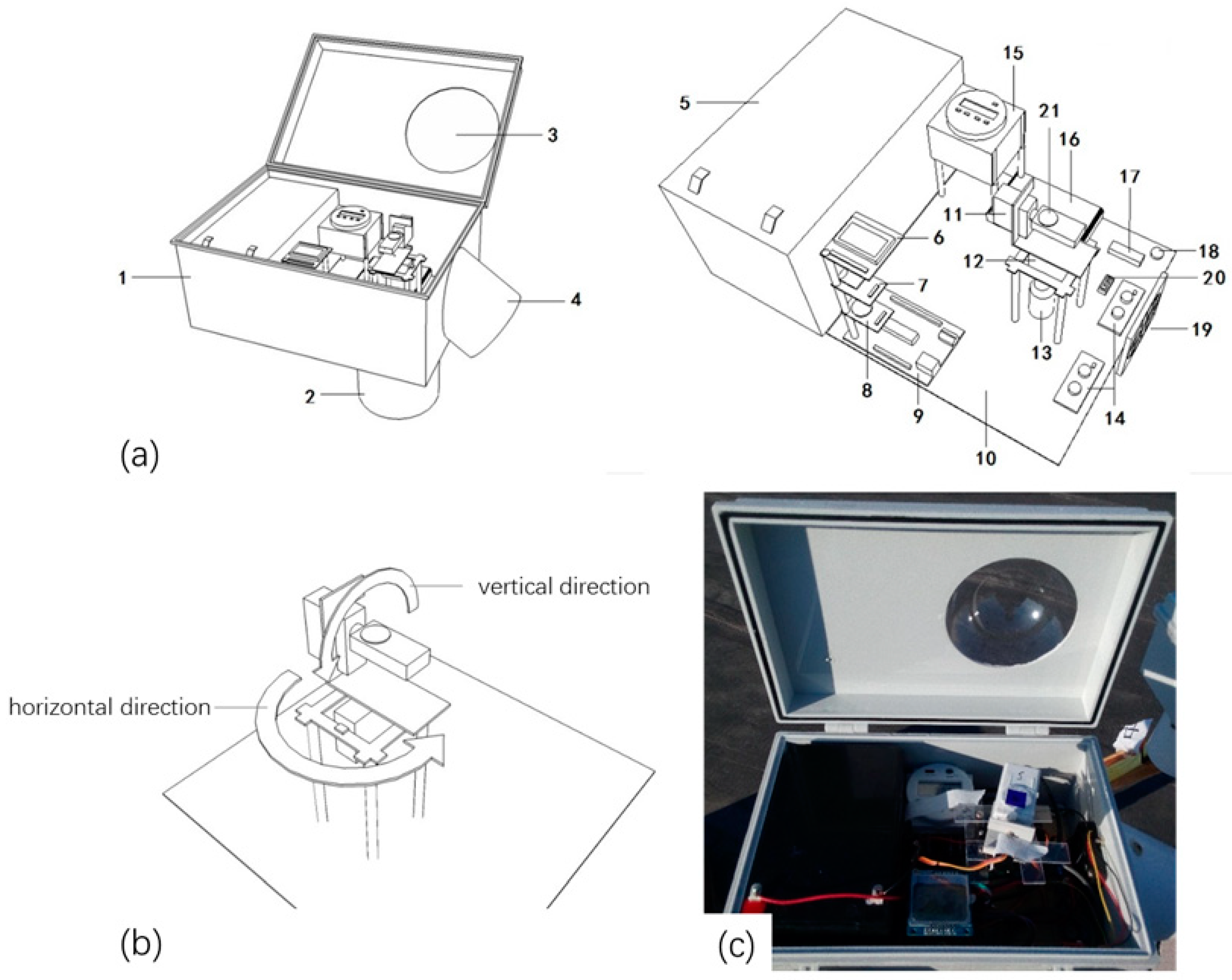
2.2. Instrument Design

The AHS consists of three main parts: the solar energy system, the timer module, and a controlling system. The diagram of the AHS is shown in Figure 1a. The solar energy system consists of a 50 W solar panel (GHM-50, GUANGHE Ltd., Changsha, China), a 12 AH accumulator battery (GHY6012, GUANGHE Ltd., Changsha, China), and a solar charge controller (GH808, GUANGHE Ltd., Changsha, China). The power supplement period of the accumulator battery is controlled by a timer (CN102A, SoarJin Co., Ltd., Wenzhou, China) to decrease the power consumption when the AHS is in standby mode. A chip (Arduino UNO R3, Arduino, MONZA, Italy) is the core component of the central system for controlling the movement of the servomotor, the function of the optical sensor, and other modules. There are some other auxiliary components, such as the screen module (Nokia 5110 LCD, Nokia Corp., Espoo, Finland), the SD card module (MicroSD Card Adapter module, CATALEX Co., Ltd., Shenzhen, China), the clock module (DS1307, CATALEX Co., Ltd., Shenzhen, China), and temperature/humidity sensors (AM2305, LEXIANG Co., Ltd., Conton, China). An ambient light sensor (BH1750FVI, ROHM Co., Ltd., Kyodo, Japan) is rotated hemispherically by a pair of PWM digital servomotors (DS215MG, KST Ltd., Meizhou, China), which are stepper motors. The single chip was programmed using the ArduinoIDE programming language so that after the vertical servomotor rotates to the specified angle, the horizontal servomotor rotates in seven directions, and the vertical servomotor enters the next cycle. The ambient light sensor, which can achieve enough multi-directional scanning of the incoming light intensity to cover the entire hemisphere, was used instead of a fisheye optical sensor. Temperature and humidity are detected every time the light intensity is observed for further analyses, such as carbon fixation, climate change, and feedback to the climate system. The data are stored in the SD card in a txt file labeled with the time (i.e., MMDDHHMM.txt).

To calculate light penetration through the canopy based on Beer’s law (Equation (1)), foliage is treated as a black body. Since foliage strongly absorbs blue light, it can be considered to be optically black in the visible wavelength range, although weak blue light scattering could induce the underestimation of PAI by up to 15%. An optical low-pass filter (<500 nm) for the blue band (QB29, Yongxing Information Sensing Technology Co., Ltd., Beijing, China) was thus placed above the chamber containing the ambient light sensor in the AHS. The azimuth angle ranged from 0 to 150° at 25° intervals, and the zenith angle ranged from 0 to 60° at 10° intervals (Figure 1b).

When used to obtain the gap fraction, one AHS was placed under the canopy to observe the transmitted light intensity through the canopy (named the “below-canopy” value hereafter). The other one was placed in an open field near the forest to detect the original light intensity (named the “above-canopy” value hereafter). By taking the ratio of the below-canopy value to the above-canopy value, the gap fraction of the canopy can be directly obtained. Compared with digital hemispherical photography, the AHS avoids the need for setting the photographic exposure and post-image classification, both of which can create considerable errors in differentiating between sky and foliage pixels.

2.3. Proof-of-Concept Experiment

Four AHSs were made to detect the PAI_e continuously. The spatial light intensity scanned by the ambient light sensor was driven by two servomotors, which were programmed by a single chip. One servomotor rotated horizontally within the azimuth angle range from 0 to 150° at 25° intervals (seven readings were made within one rotation). The other rotated vertically within the zenith angle range from 0 to 60° at 10° intervals immediately after the horizontal rotation was completed. A complete hemispherical scan therefore created a 7 × 7 data matrix. The measurement of the 7 × 7 matrix took 50 s. The georeferenced value depends on the azimuth angle of the instrument. No noise was generated by the motors, but other factors may have caused noise, such as leaves shaking when the servomotors completed the measurement rotation, which was small and negligible during the test. All the AHSs were placed on the tripod and maintained in a horizontal position.

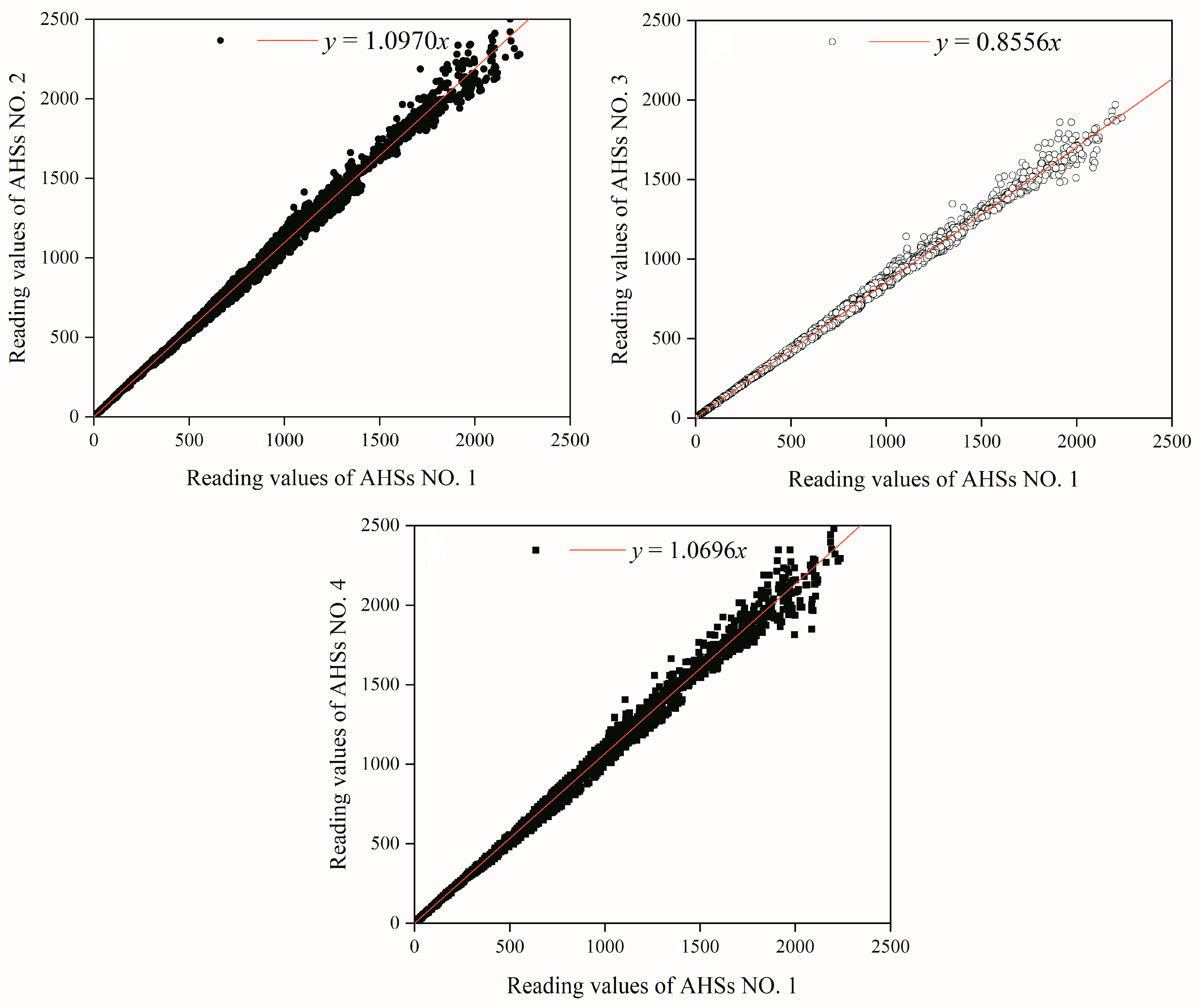
2.3.1. Instrument Calibration

In order to obtain the gap fraction (P(θ)) for calculating PAI_e (Equation (3)), at least two AHSs are required to measure the light intensity above and below the canopy simultaneously. However, differences between the light sensors on different AHSs can influence the accuracy of the measurement, which should be eliminated by mutual calibration of the instruments before the field measurement. To remove the differences between AHSs, four AHSs were placed side by side in an open field and operated simultaneously. Taking the readings from one AHS as the standard, the readings from the other three AHSs were corrected to the standard through linear regression.

2.3.2. Investigation of Observation Conditions

According to Beer’s law, PAI_e can be accurately calculated by the canopy gap fraction only under a diffuse sky with moderate irradiance conditions. A clear sky with strong direct radiation casts sunflecks that enhance the spatial heterogeneity in the radiation transferred through the forest canopy, while low irradiance causes erroneous gap fraction estimates.

The effects of different sky conditions and solar radiation intensities on the PAI_e observations made by the AHS were studied through a series of field experiments in Northeast Forestry University’s Urban Forestry Demonstration Research Base. One experiment was conducted to investigate the influence of spatial heterogeneity on PAI_e estimations. One AHS was placed under the canopy with an observation direction of 45° from north to east to detect the below-canopy value, and the other one was set on open land in the same observation direction to detect the above-canopy value. The radiation intensities were logged every 30 min for 3 days, i.e., 30 April to 2 May; 30 April and 1 May were sunny days with high spatial heterogeneity in the beam radiation, and 2 May was cloudy with relatively homogeneous beam radiation.

Another experiment was conducted to investigate the influence of irradiance intensity on the PAI_e measurements. One AHS was placed under a potted plant tree to simulate the below-canopy value, and the other one was placed in an open field near the first one to detect the above-canopy value under different irradiance intensities. Thus, a series of PAI_e values could be calculated. As the radiance intensity varied with time, the relationship between PAI_e and radiance intensity could be obtained.

As hypothesized, the PAI_e tended to be unstable with a decrease in radiance intensity. By comparing the ratios of the below-canopy to the above-canopy values of light intensity in different irradiance environments, the sensitivity of the gap fraction to irradiance intensity can be quantified.

2.3.3. Comparison with the Commercial LAI-2200 Instrument

In order to test the performance of the AHS, it was used together with an LAI-2200 to measure the PAI_e on 24 plots of a forest plantation in Northeast Forestry University’s Urban Forestry Demonstration Research Base. The main tree species in the plantation are Larix gmelinii (Rupr.) Kuzen, Pinus tabuliformis var. mukdensis Uyeki, Pinus sylvestris var. mongholica Litv., Fraxinus mandshurica Rupr., and Juglans mandshurica Maxim. The PAI_e of the tree canopy was measured using two LAI-2200 sensors. A reference sensor was placed on the roof of a building to log the above-canopy values over the canopy at 10 s intervals. The other was placed under the canopy to measure the below-canopy values. A 180° view cap was used for both LAI-2200 instruments.

2.4. Field Data

2.4.1. Study Sites

The study site was Maoershan Experimental Forest Farm of Northeast Forestry University in northeastern China (45°20′–25′ N, 127°30′–34′ E) (Figure 2e). It represents typical deciduous forests in northeastern China, with an average altitude of 300 m above sea level and an average slope of 10°–15°. The mean annual precipitation (1989–2009) is 629 mm, of which about 50% occurs between June and August. The mean annual air temperature is 3 °C. The frost-free period spans between 120 days and 140 days, with an early frost in September and a late frost in May. The study was conducted using three plots of mixed deciduous broadleaf plantations numbered Plots 1–3. Figure 2b–d present field photos of Plots 1–3.

Table 1. General characteristics and species composition of the three deciduous broadleaf forest plots.

Forest Plot	Major Species	Tree Density (ha−1)	Mean DBH (cm)	Height (m)	Slope
1	Juglans mandshurica (78.96%) Betula dahurica (17.19%)	867	16.08	17	2.7°
2	Quercus mongolica (97.61%) Ulmus japonica (1.71%)	900	19.48	21	17°
3	Quercus mongolica (47.86%) Ulmus japonica (12.69%)	1017	18.72	18	22°

Values in parentheses show the dominance of the species (i.e., the proportion of the total basal area of all species in the plot represented by the basal area of major species). DBH stands for diameter at breast height. Height is the canopy height of the dominant species in each plot.

presents detailed information about the forests studied here.

2.4.2. Data Collection

Four AHSs were used for the continuous measurement of PAI_e. Three AHSs were placed in three plots with different forest types to detect the below-canopy values, and the other was mounted in an open field near the sample plots (shown in Table 1) to measure the above-canopy values. These AHSs were all installed at 1.2 m above the ground (Figure 2b–d) on 26 April 2015. The measurements were taken at half-hourly intervals. The linear distance between the plots was less than 1 km.

2.4.3. Data Processing

The standard method implemented in the AHS is based on Equation (3). The data we obtained were not angularly continuous, so the method used in the LAI-2000 plant canopy analyzer (i.e., computing PAI_e from Equation (3) by discrete summation over the five zenith view angles) was adopted for data processing. LAI-2200 was used in the same data collection campaigns. The difference was that the AHS has seven rather than five zenith view angles. Compared with LAI-2000, the view did not cover the full 90° range to meet the conditions of Equations (4) and (5).

As the AHS is designed to operate continuously for a whole growing season and to log data every 30 min, the amount of data to be stored is large. All the processes of data collection, data matching the above-canopy and below-canopy values, selecting the transmittance values, and calculation were automatically completed by programming in MATLAB. The list of experiments described above is presented in

Table 2. Experiment descriptions.

Experiment	Experimental Place	Comments
Influence of the spatial heterogeneity of radiation on PAIe estimation	Northeast Forestry University’s Urban Forestry Demonstration Research Base	Investigation of observation conditions
Influence of radiation intensity on estimations of PAIe	Northeast Forestry University’s Urban Forestry Demonstration Research Base	Investigation of observation conditions
Comparison with the LAI-2200 plant canopy analyzer	Northeast Forestry University’s Urban Forestry Demonstration Research Base	Accuracy verification
Field experiment	Maoershan Experimental Forest Farm	Monitoring the leaf area index of forest canopies

.

3. Results

3.1. Lab Experiment

3.1.1. Instrument Calibration

In total, 3235 groups of data ranging from 0 to 2600 (no unit) were obtained to analyze the variations among the four instruments we assembled. Taking the data from AHS No. 1 as the reference, the data from AHS No. 2, No. 3, and No. 4 are shown in Figure 3. The deviation between the different AHSs showed a significant linear trend, with all R² values being above 0.99. When a canopy gap fraction was calculated by the ratio of below-canopy to above-canopy values, the data from different AHSs were calibrated according to the linear regression results shown in Figure 3.

3.1.2. Influence of the Spatial Heterogeneity of Radiation on PAI Estimation

An experiment to study the influence of the spatial heterogeneity of radiation on PAI_e was conducted at a plot at the Northeast Forestry University in April and May of 2014. Data from 3 days (30 April, 1 May, and 2 May) were chosen from 2 months of data to explore the influence of the spatial heterogeneity of irradiance on PAI_e estimation; 30 April and 1 May were sunny days, and 2 May was a cloudy day with diffuse sky conditions. The PAI_e obtained during this period is shown in Figure 4a. The PAI_e from 2 May was substantially more stable than that from the other two sunny days. According to previous research by Hyer and Goetz [34], the PAI_e obtained from multi-angled methods is relatively accurate when detected under diffuse sky conditions. Here, we demonstrated that strong beam radiation and sunflecks enhanced the spatial heterogeneity of ambient forest light and caused fluctuations in the PAI_e on 30 April and 1 May.

The data for the above-canopy values were chosen for further analysis. The standard deviations of seven azimuth radiation intensities from the same zenith angle and the same batch were calculated. The mean value of the standard deviations from the seven zenith angles and the mean value of all 49 radiation intensities were calculated and are shown in Figure 4b. This figure shows that the mean intensity reached a peak at noon and that the standard deviations of 30 April and 1 May (both sunny days) were substantially higher than that of the cloudy day. These conclusions could guide the choice of transmittance values for accurate calculations of PAI_e in subsequent algorithms.

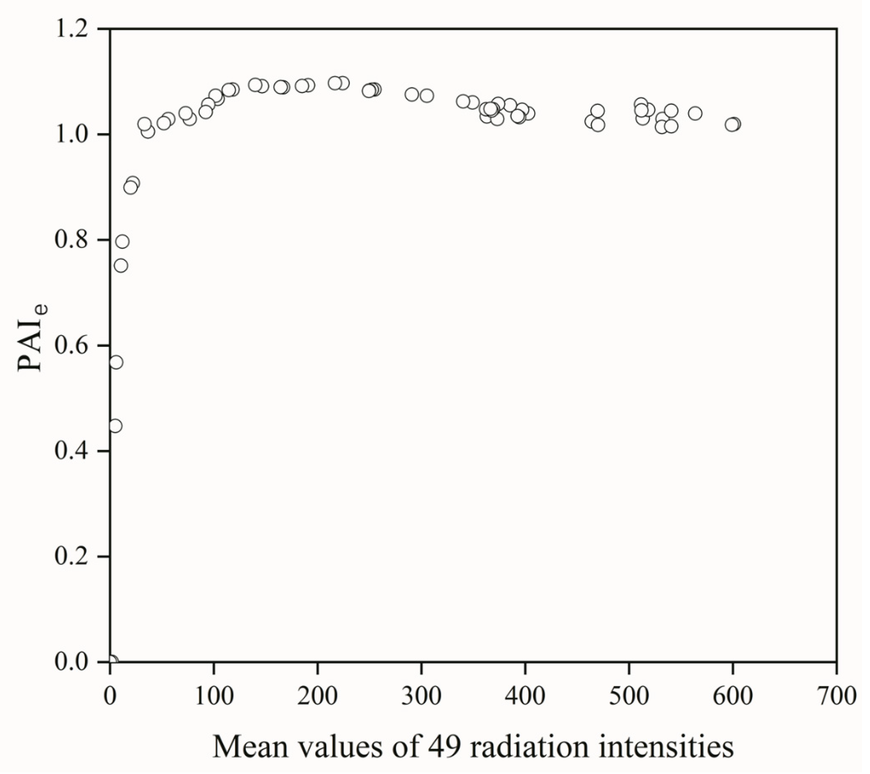
3.1.3. Influence of Radiation Intensity on Estimations of PAI_e

Gap fraction measurements under low irradiance are generally inaccurate. An experiment to detect the sensitivity of PAI_e to irradiance intensity was conducted on 24 September 2014 in overcast conditions to guarantee low spatial heterogeneity in a light environment. One AHS was placed on open land, and the other was settled under the potted plant tree to simulate the light transmitted through foliage in the forest. The light intensity was observed every 5 min. The PAI_e values under different light intensities were calculated, and the relationships between the mean values of light intensity and the corresponding PAI_e are shown in Figure 5. It is obvious that the PAI_e tends to be unstable with decreasing radiation intensity. Therefore, during the calculation of seasonal PAI_e, irradiance intensity should be considered to select transmittance values for accurate PAI_e estimation. Moreover, randomly distributed foliage is seldom encountered in real situations, but such uncertainty is still controlled because the light intensity has a greater impact on the experiment.

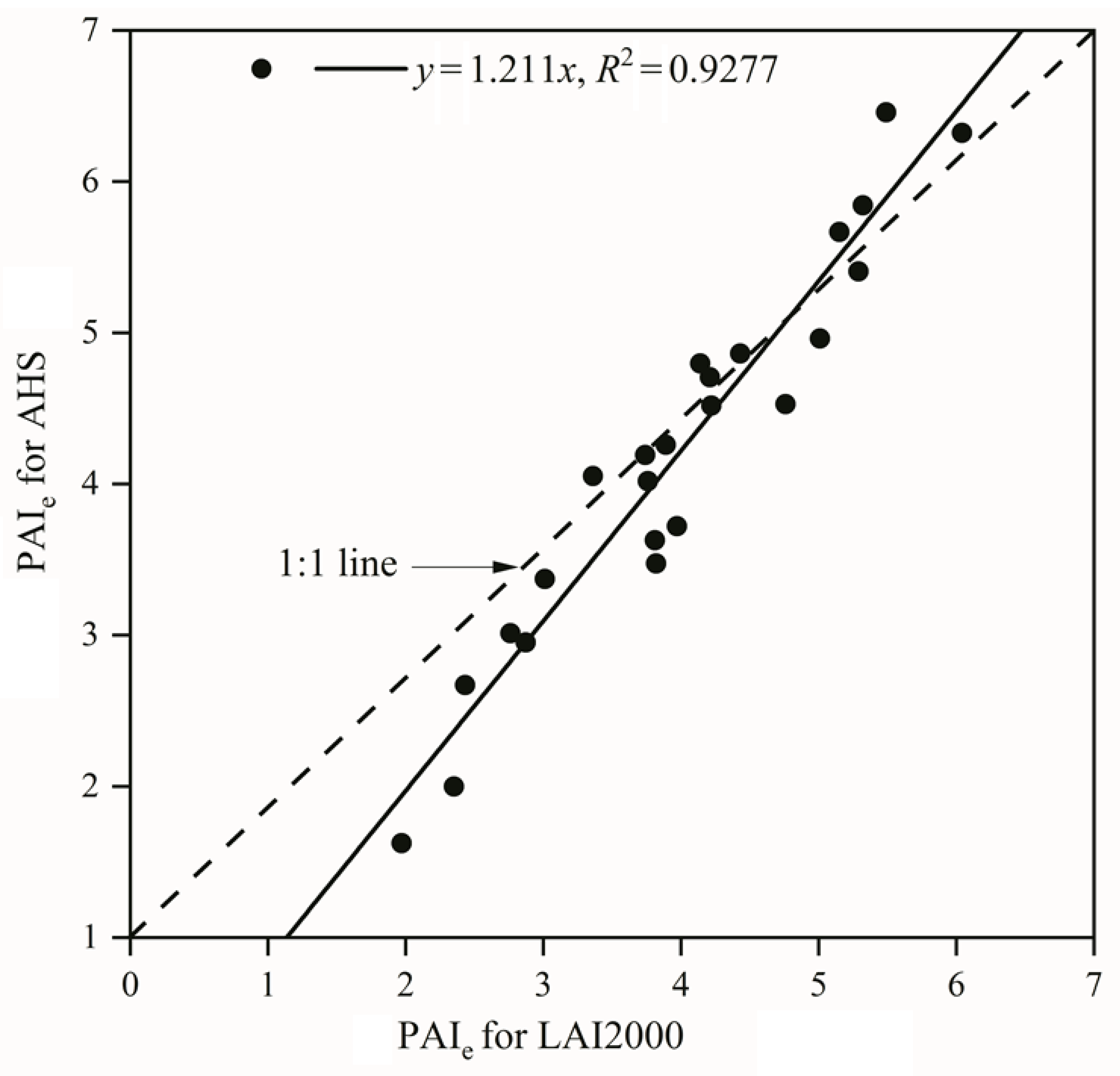
3.1.4. Comparison with the LAI-2200 Plant Canopy Analyzer

A commercial product (LAI-2200) for PAI_e detection was applied in our experiment and compared with the results of the AHS. These two instruments were both placed in 24 plots and kept in the same observation direction. The comparison of these results is shown in Figure 6. PAI_e ranged from 1.5 to 6.5, the correlation between the PAI_e from the LAI-2200 and the PAI_e from the AHS was high with an R² of 0.9277, and the root mean square error was 0.41.

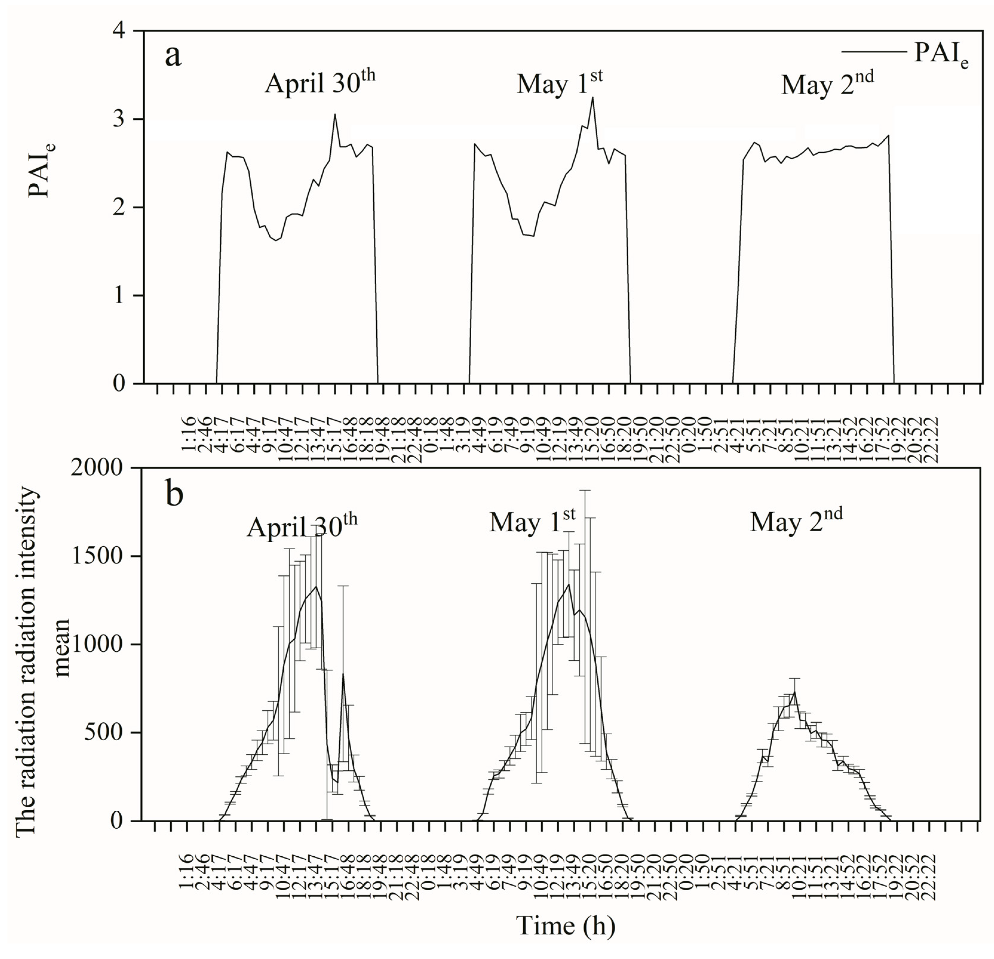
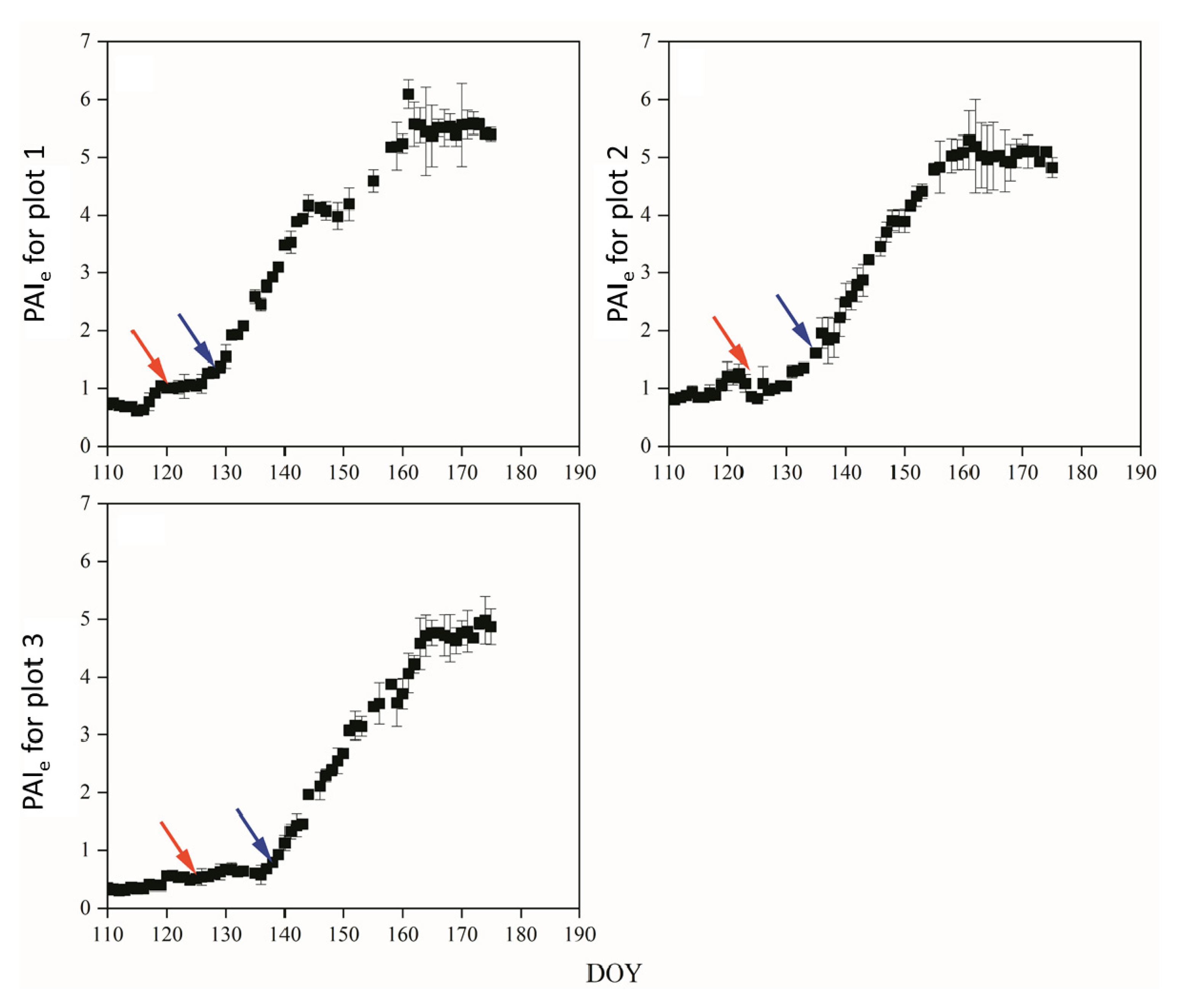
3.2. Field Experiment

Four AHSs were placed in Maoershan Experimental Forest Farm in the spring of 2015 before leaf-out. Three of them were placed in plots with three forest types, and one AHS was placed in open land to measure the radiation intensity as the above-canopy value. Forty-eight groups of data could be obtained from one AHS every day. The transmittance values were chosen according to the principles mentioned in Section 3.1.2 and Section 3.1.3 and applied to calculate the PAI_e by the gap fraction method. The mean and standard deviation of PAI_e calculated from the transmittance values are shown in Figure 7. Data for day of year (DOY) 139, 150, 159, and 162 were missed owing to continuous rain, and the data for DOY 153, 155, 158, and 161 were missed owing to the battery being low. The proportion of missing data for the three AHSs was 11.9%, 5.9%, and 5.9%. At the initial stage of observation, the PAI_e we obtained was mainly caused by the branches and trunks, because the trees had not sprouted; this could be interpreted as the effective woody area index (WAI_e). The WAI_e values of Plots 1, 2, and 3 were stable at around 0.353, 0.724, and 0.864, respectively. The first increase seen in the three sample plots (detected when the shrubs spread their leaves, shown as red arrows) occurred on DOY 125, 121, and 124, respectively. The second increase seen in the three sample plots (shown as blue arrows) occurred on DOY 142, 133, and 137, respectively. The full leaf-out dates were DOY 171, 167, and 166 with peak PAI_e values of 5.57, 5.3, and 4.93 in the three experiment plots, respectively.

4. Discussion

Leaf area index (LAI) products are now routinely generated by remote sensing and are widely used in most land surface process models. Assessing the uncertainties associated with these LAI products is essential for their proper application [34,35,36,37]. LAI can be determined by direct methods in the field [12]. The advantage of direct methods such as the LAI-2000 Plant Canopy Analyzer or its updated version (LAI-2200) is that they can obtain accurate results, while their disadvantages are that measurements are time-consuming, costly, and not repeatable in some circumstances [10,15]. During our experiment, a novel instrument, the AHS, was developed to measure PAI_e for monitoring daily changes in LAI in forest ecosystems. In contrast to previous studies, the AHS can achieve non-destructive measurements that are inexpensive, convenient, and rapid.

The design of the AHS was studied. An optical sensor driven by a pair of servomotors was used to observe hemispherical light transmission continuously at adjustable intervals, and a blue filter was used to reduce the multiple scattering effect of light on the transmission measurements. Moreover, a set of algorithms was developed. The measurements of the AHS are based on Beer’s law. The incident irradiance, canopy structure, and optical properties all influence the total amount of radiation intercepted by canopy layers [15]. When Beer’s law is applied to model light extinction in vegetation canopies [38], foliage elements are considered to be absolutely absorbing (the black body assumption) [39]. Blue light seems to be the optimal light due to its high transmittance through the atmosphere and its low reflectance through foliage [40]. Therefore, a blue filter was placed in front of the sensor to improve the accuracy of detection. Obtaining the optimal daily PAI_e data is the key point in obtaining the seasonal PAI_e during long-term detection. According to our previous experience with optical instruments, two light conditions were mainly considered in order to reduce noise in the daily PAI_e estimations. In our experiment, one condition was diffuse sky conditions, because the heterogeneity of light could increase the light intensity in certain directions and lead to an inaccurate PAI_e. The deviation in radiation density should be lower than 150. The other was a moderate irradiance condition, because too little irradiance could decrease the sensitivity of gap fraction estimates, and the mean values of radiation density should be higher than 80. The PAI_e could be estimated under these circumstances.

The PAI data for typical days were used to study the influence of the spatial heterogeneity of radiation on effective PAI detection. One AHS was settled horizontally in the plot; the other was settled on a rooftop near the plot in the same observation direction. The PAI_e from 2 May (a cloudy day) was significantly more stable than that from the other two days (30 April and 1 May, which were sunny days with high spatial heterogeneity of radiation) because of the diffuse illuminance. Most PAI_e values were above zero, and the average and standard deviation were 2.64 and 0.75, respectively. As illustrated in Figure 4a, most data from 30 April and 1 May, with strong sunlight, were significantly different from those of 2 May. This led to a larger gap fraction and a lower PAI_e than the real values. Under these conditions, the estimated PAI_e observed on 30 April and 1 May could be 38.59% and 36.67% lower than that under diffuse conditions at the largest extent, respectively. However, when the beam direction is within the scanning scope of the instrument, the above-canopy value would be significantly higher, making the ratio of the below-canopy value to the above-canopy value much lower compared with that under diffuse sky conditions. In this situation, the estimated gap fraction would be lower and the PAI_e would be higher than their real values.

The mean and standard deviation of light intensity above the canopy from different directions are shown in Figure 4b. The difference in the light intensity from different directions was more substantial under strong sunshine than on cloudy days or under weak sunshine. Thus, the standard deviation was chosen as an index to distinguish diffuse sky conditions. The influence of low irradiance on PAI_e detection is shown in Figure 5. The PAI_e became unstable with decreasing light intensity. Low ambient light intensity could intensify the error of the gap fraction and result in a low PAI_e. The PAI_e of 2 May at 4:20 (24 h) in the last experiment considering the spatial heterogeneity of radiation was low because of the low ambient light intensity when the sun rose on a cloudy day.

The PAI_e data for Maoershan Experimental Forest Farm from the leaf-out to full-leaf period were detected and are shown in Figure 7. The gap fractions obtained by the AHS were based on an optical sensor, so the contributions of leaves and branches were involved. At the initial stage after the AHSs were placed, the data we obtained could be considered as the woody area index (WAI_e). It is worth mentioning that during our studies, the woody materials were assumed to stop growing during a year, or the variation in WAI_e is negligible. In real situations, such uncertainties should be taken into consideration. The PAI_e data after leaf-out minus WAI_e could easily eliminate the error in the LAI_e calculations caused by tree branches [41]. The PAI_e for three plots on DOY 125, 121, and 124 increased significantly. As reported in other temperate deciduous forests, the understory canopy unfolded leaves earlier than the overstory canopy [42,43]. We speculate that the increase in PAI_e during this period was caused by the new leaves unfolding in the understory canopy. This increasing trend lasted for 3 to 4 days at a relatively slow rate. The PAI_e exhibited another significant increase (more than 3) on DOY 171, 167, and 166 and reached peaks of 4.93, 5.57, and 5.3 for the three plots, respectively. This increasing trend was caused by the unfolding of the overstory canopy.

High-frequency daily PAI_e from the three plots during the spring were obtained and used to analyze the phenological metrics. On the basis of the observed data, we found that the phenological properties varied in the three plots. This finding highlights the importance of quantifying uncertainty in phenological metrics through high-frequency observations. Auto-observation instruments could obtain high-frequency data and reduce errors caused by duplicated measurements compared with manual operations [44]. There are advantages and disadvantages for all kinds of instruments. Thus, it was important to use multiple instruments and compare their PAI estimates [20]. The AHS could inspire some other novel instrument designs as a reference or provide the basic data for LAI intercomparisons with other instruments.

Overall, the LAI-2200 and the AHS obtained similar PAI_e estimations. The PAI_e values measured by the LAI-2200 were higher than those of the AHS when the values were lower than 4 (Figure 6). Moreover, a complete scan takes about 50 s, and the accuracy will be affected by the cause of any variance in the field measurement, such as wind moving the branches during a scan; this was also one of the uncertainties in our field experiment. Furthermore, dust accumulating on the instrument could potentially affect the measurements. During our experiment, a protective dark shell with a steering gear control on the outermost layer was added to the new instrument, which was only opened during the measurements. The above-canopy sensor may degrade at a faster rate than the below-canopy one, which has less UV exposure due to shading by the canopy, especially in coniferous forests, and pine oil drops also affected the measurements. Therefore, our improvement plan is to overcome these setbacks, which would be very practical for deploying such methods.

PAI estimations based on the gap fraction require the light intensity from a particular direction (e.g., 57°) or multiple directions [9]. Fisheye photography is commonly used in multi-direction observations [45,46,47]. As far as we know, no study has reported servomotors driving a passive optical sensor for continuous multi-angle PAI observations, followed by calculating the PAI. We believe that our instrument is the first servomotor-driven optical sensor for continuous multiple-angled LAI observation. Compared with photographic techniques, there are some advantages of the AHS: (1) the optical sensor has a lower cost than a camera; (2) the data from the AHS are significantly smaller than those of a camera and are more efficient for wireless transmission (this advantage could be more obvious if applied with GPRS transmission in the future); (3) the scanning track controlled by a single chip is more flexible and not limited to several zenith angles or points; (4) AHS based on a single chip could be implemented to assemble more modules to detect more indices besides LAI, such as temperature and humidity. In the future, a GPRS internet module could be added to achieve the synchronous transmission of data.

Webcam-based phenology monitoring networks have advanced in recent years [34,38]. Most webcams are mounted on towers, resulting in oblique or horizontal views to include maximum canopy coverage in the images [48,49,50,51,52,53,54]. This setting has merits when monitoring canopy phenology. The low cost, small data size, simple arithmetic, and possibility for flexible modification of the AHS are suitable for ground-based phenology monitoring networks designed to determine the phenological characteristics of more types of forest, and thus the AHS has high potential for commercial applications. In future research, the scanning system, which only extends to an azimuth of 150 degrees, could be limited in terms of angular observations; therefore, a full 360-degree azimuth range should be developed to obtain more accurate results.

5. Conclusions

A novel instrument, the AHS, for monitoring the phenology of forest canopies was designed. The optical sensor driven by a pair of servomotors was able to obtain the light intensity from multiple directions to calculate the gap fraction and LAI. Proof-of-concept experiments were designed to improve the accuracy of LAI measurements from the perspectives of diffusion sky conditions and moderate irradiance intensity. After correction of the differences between the AHSs and the addition of a blue filter, the gap fraction became more accurate. The research results for the AHS agreed well with the results obtained using the LAI-2200 plant canopy analyzer. The AHS was applied in a field test of three forest types, and it proved to be a high-frequency, automated, low-cost, stable, easily constructed, and flexibly modified instrument for phenological studies. In future research, instruments with a wider range of view angles should be developed to obtain more accurate results, and instrument protective shells should be added to obtain long-term and accurate monitoring LAI data.

References

1. Chen, J.M.; Black, T.A. Foliage area and architecture of clumped plant canopies from sunfleck size distributions. Agric. For. Meteorol. 1992, 60, 249–266. [Google Scholar] [CrossRef]
2. Asner, G.P.; Scurlock, J.M.O.; Hicke, J.A. Global synthesis of leaf area index observations: Implications for ecological and remote sensing studies. Glob. Ecol. Biogeogr. 2003, 12, 191–205. [Google Scholar] [CrossRef]
3. Ryu, Y.; Fang, H.L.; Claverie, M.; Myneni, R.; Zhu, Z. Inconsistencies of interannual variability and trends in long-term satellite leaf area index products. Glob. Chang. Biol. 2017, 23, 4133–4146. [Google Scholar]
4. Leuning, R.; Kelliher, F.M.; Pury, D.G.G.D.; Schulze, E.D. Leaf nitrogen, photosynthesis, conductance and transpiration: Scaling from leaves to canopies. Plant Cell Environ. 1995, 18, 1183–1200. [Google Scholar] [CrossRef]
5. Lindner, S.; Wei, X.; Nay-Htoon, B.; Choi, J.; Ege, Y.; Lichtenwald, N.; Fischer, F.; Ko, J.; Tenhunen, J.; Otieno, D. Canopy scale CO2 exchange and productivity of transplanted paddy and direct seeded rainfed rice production systems in S. Korea. Agric. For. Meteorol. 2016, 228–229, 229–238. [Google Scholar] [CrossRef]
6. Chen, J.M.; Liu, J.; Cihlar, J.; Goulden, M.L. Daily canopy photosynthesis model through temporal and spatial scaling for remote sensing applications. Ecol. Model. 1999, 124, 99–119. [Google Scholar] [CrossRef]
7. Fotis, A.T.; Morin, T.H.; Fahey, R.T.; Hardiman, B.S.; Bohrer, C. Forest structure in space and time: Biotic and abiotic determinants of canopy complexity and their effects on net primary productivity. Agric. For. Meteorol. 2018, 250–251, 181–191. [Google Scholar] [CrossRef]
8. Savoy, P.; Mackay, D.S. Modeling the seasonal dynamics of leaf area index based on environmental constraints to canopy development. Agric. For. Meteorol. 2015, 200, 46–56. [Google Scholar] [CrossRef]
9. Gonsamo, A.; Walter, J.M.; Chen, J.M.; Pellikka, P.; Schleppi, P. A robust leaf area index algorithm accounting for the expected errors in gap fraction observations. Agric. For. Meteorol. 2017, 248, 197–204. [Google Scholar] [CrossRef]
10. Liu, Z.; Chen, J.M.; Jin, G.; Qi, Y. Estimating seasonal variations of leaf area index using litterfall collection and optical methods in four mixed evergreen–deciduous forests. Agric. For. Meteorol. 2015, 209–210, 36–48. [Google Scholar] [CrossRef]
11. Ryu, Y.; Verfaillie, J.; Macfarlane, C.; Kobayashi, H.; Sonnentag, O.; Vargas, R.; Ma, S.; Baldocchi, D.D. Continuous observation of tree leaf area index at ecosystem scale using upward-pointing digital cameras. Remote Sens. Environ. 2012, 126, 116–125. [Google Scholar] [CrossRef]
12. Küssner, R.; Mosandl, R. Comparison of direct and indirect estimation of leaf area index in mature Norway spruce stands of eastern Germany. Can. J. For. Res. 2000, 30, 440–447. [Google Scholar] [CrossRef]
13. Breda, N.J. Ground-based measurements of leaf area index: A review of methods, instruments and current controversies. J. Exp. Bot. 2003, 54, 2403–2417. [Google Scholar] [CrossRef]
14. Chen, J.M.; Plummer, P.S.; Rich, M.; Gower, S.T.; Norman, J.M. Leaf area index measurements. J. Geophys. Res. 1997, 102, 29429–29443. [Google Scholar] [CrossRef]
15. Jonckheere, I.; Fleck, S.; Nackaerts, K.; Muys, B.; Coppin, P.; Weiss, M.; Baret, F. Review of methods for in situ leaf area index determination: Part I. Theories, sensors and hemispherical photography. Agric. For. Meteorol. 2004, 121, 19–35. [Google Scholar] [CrossRef]
16. Sprintsin, M.; Cohen, S.; Maseyk, K.L.; Rotenberg, E.; Grünzweig, J.; Karnieli, A.; Berliner, P.; Yakir, D. Long term and seasonal courses of leaf area index in a semi-arid forest plantation. Agric. For. Meteorol. 2011, 151, 565–574. [Google Scholar] [CrossRef]
17. Wang, R.; Chen, J.M.; Liu, Z.; Arain, A. Evaluation of seasonal variations of remotely sensed leaf area index over five evergreen coniferous forests. ISPRS J. Photogramm. Remote Sens. 2017, 130, 187–201. [Google Scholar] [CrossRef]
18. Fan, X.; Kawamura, K.; Xuan, T.D.; Yuba, N.; Lim, J.; Yoshitoshi, R.; Minh, T.N.; Kurokawa, Y.; Obitsu, T. Low-cost visible and near-infrared camera on an unmanned aerial vehicle for assessing the herbage biomass and leaf area index in an Italian ryegrass field. Grassl. Sci. 2017, 64, 145–150. [Google Scholar] [CrossRef]
19. Richardson, A.D.; O’Keefe, J. Phenological Differences between Understory and Overstory; Springer: New York, NY, USA, 2009; pp. 87–117. [Google Scholar]
20. Brown, L.A.; Ogutu, B.O.; Dash, J. Tracking forest biophysical properties with automated digital repeat photography: A fisheye perspective using digital hemispherical photography from below the canopy. Agric. For. Meteorol. 2020, 287, 107944. [Google Scholar] [CrossRef]
21. Qu, Y.; Han, W.; Fu, L.; Li, C.; Song, J.; Zhou, H.; Bo, Y.; Wang, J. LAINet–A wireless sensor network for coniferous forest leaf area index measurement: Design, algorithm and validation. Comput. Electron. Agric. 2014, 108, 200–208. [Google Scholar] [CrossRef]
22. Brede, B.; Gastellu-Etchegorry, J.; Lauret, N.; Baret, F.; Clevers, J.G.P.W.; Verbeselt, J.; Herold, M. Monitoring Forest Phenology and Leaf Area Index with the Autonomous, Low-Cost Transmittance Sensor PASTiS-57. Remote Sens. 2018, 10, 1032. [Google Scholar] [CrossRef] [Green Version]
23. Niu, X.; Fan, J.; Luo, R.; Fu, W.; Yuan, H.; Du, M. Continuous estimation of leaf area index and the woody-to-total area ratio of two deciduous shrub canopies using fisheye webcams in a semiarid loessial region of China. Ecol. Indic. 2021, 215, 107549. [Google Scholar] [CrossRef]
24. Toda, M.; Richardson, A.D. Estimation of plant area index and phenological transition dates from digital repeat photography and radiometric approaches in a hardwood forest in the Northeastern United States. Agric. For. Meteorol. 2018, 249, 457–466. [Google Scholar] [CrossRef]
25. Chianucci, F.; Bajocco, S.; Ferrara, C. Continuous observations of forest canopy structure using low-cost digital camera traps. Agric. For. Meteorol. 2021, 307, 108516. [Google Scholar] [CrossRef]
26. Ryu, Y.; Baldocchi, D.D.; Verfaillie, J.; Ma, S.; Falk, M.; Ruiz-Mercado, I.; Hehn, T.; Sonnentag, O. Testing the performance of a novel spectral reflectance sensor, built with light emitting diodes (LEDs), to monitor ecosystem metabolism, structure and function. Agric. For. Meteorol. 2011, 150, 1597–1606. [Google Scholar] [CrossRef]
27. Culvenor, D.S.; Newnham, G.J.; Mellor, A.; Sims, N.C.; Haywood, A. Automated In-Situ Laser Scanner for Monitoring Forest Leaf Area Index. Sensors 2014, 14, 14994–15008. [Google Scholar] [CrossRef]
28. Chen, J.M.; Black, T.A. Defining leaf area index for non-flat leaves. Plant Cell Environ. 1992, 15, 421–429. [Google Scholar] [CrossRef]
29. Leblanc, S.G.; Chen, J.M.; Fernandes, R.; Deering, D.W.; Conley, A. Methodology comparison for canopy structure parameters extraction from digital hemispherical photography in boreal forests. Agric. For. Meteorol. 2005, 129, 187–207. [Google Scholar] [CrossRef]
30. Ryu, Y.; Sonnentag, O.; Nilson, T.; Vargas, R.; Kobayashi, H.; Wenk, R.; Baldocchi, D.D. How to quantify tree leaf area index in an open savanna ecosystem: A multi-instrument and multi-model approach. Agric. For. Meteorol. 2010, 150, 63–76. [Google Scholar] [CrossRef]
31. Liang, A.R.G.; Yueqin, X. Estimation of leaf area index from transmission of direct sunlight in discontinuous canopies. Agric. For. Meteorol. 1986, 37, 229–243. [Google Scholar] [CrossRef]
32. Miller, J.B. A formula for average foliage density. Aust. J. Bot. 1967, 15, 141–144. [Google Scholar] [CrossRef]
33. Welles, J.M.; Norman, J.M. Instrument for Indirect Measurement of Canopy Architecture. Agron. J. 1991, 83, 818–825. [Google Scholar] [CrossRef]
34. Hyer, E.J.; Goetz, S.J. Comparison and sensitivity analysis of instruments and radiometric methods for LAI estimation: Assessments from a boreal forest site. Agric. For. Meteorol. 2004, 122, 157–174. [Google Scholar] [CrossRef]
35. Woodgate, W.; Jones, S.D.; Suarez, L.; Hill, M.J.; Armston, J.D.; Wilkes, P.; Soto-Berelov, M.; Haywood, A.; Mellor, A. Understanding the variability in ground-based methods for retrieving canopy openness, gap fraction, and leaf area index in diverse forest systems. Agric. For. Meteorol. 2015, 205, 83–95. [Google Scholar] [CrossRef]
36. Yin, Y.; Ma, D.; Wi, S.; Dai, E.; Zhu, Z.; Myneni, R.B. Nonlinear variations of forest leaf area index over China during 1982–2010 based on EEMD method. Int. J. Biometeorol. 2016, 61, 977–988. [Google Scholar] [CrossRef] [PubMed]
37. Gonsamo, A.; Pellikka, P. The sensitivity based estimation of leaf area index from spectral vegetation indices. ISPRS J. Photogramm. Remote Sens. 2012, 70, 15–25. [Google Scholar] [CrossRef]
38. Verger, A.; Filella, I.; Baret, F.; Peñuelas, J. Vegetation baseline phenology from kilometric global LAI satellite products. Remote Sens. Environ. 2016, 178, 1–14. [Google Scholar] [CrossRef]
39. Palmeri, L.; Barausse, A.; Jorgensen, D.S.E. Ecological Processes Handbook; CRC Press: Boca Raton, FL, USA, 2013; pp. 87–117. [Google Scholar]
40. Garrigues, S.; Shabanov, N.V.; Swanson, K.; Morisette, J.T.; Baret, F.; Myneni, R.B. Intercomparison and sensitivity analysis of Leaf Area Index retrievals from LAI-2000, AccuPAR, and digital hemispherical photography over croplands. Agric. For. Meteorol. 2008, 148, 1193–1209. [Google Scholar] [CrossRef]
41. Brusa, A.; Bunker, D.E. Increasing the precision of canopy closure estimates from hemispherical photography: Blue channel analysis and under-exposure. Agric. For. Meteorol. 2014, 195–196, 102–107. [Google Scholar] [CrossRef]
42. Chen, J.M. Optically-based methods for measuring seasonal variation of leaf area index in boreal conifer stands. Agric. For. Meteorol. 1996, 80, 135–163. [Google Scholar] [CrossRef]
43. Richardson, A.D.; Jenkins, J.P.; Braswell, B.H.; Hollinger, D.Y.; Ollinger, S.V.; Smith, M.L. Use of digital webcam images to track spring green-up in a deciduous broadleaf forest. Oecologia 2007, 152, 323–334. [Google Scholar] [CrossRef] [PubMed]
44. Seiwa, K. Advantages of early germination for growth and survival of seedlings of Acer mono under different overstorey phenologies in deciduous broad-leaved forests. J. Ecol. 2010, 86, 219–228. [Google Scholar] [CrossRef]
45. Ryu, Y.; Lee, G.; Jeon, S.; Song, Y.; Kimm, H. Monitoring multi-layer canopy spring phenology of temperate deciduous and evergreen forests using low-cost spectral sensors. Remote Sens. Environ. 2014, 149, 227–238. [Google Scholar] [CrossRef]
46. Macfarlane, C.; Ryu, Y.; Ogden, G.N.; Sonnentag, O. Digital canopy photography: Exposed and in the raw. Agric. For. Meteorol. 2014, 197, 244–253. [Google Scholar] [CrossRef]
47. Yin, G.; Li, A.; Jin, H.; Zhao, W.; Bian, J.; Qu, Y.; Zeng, Y.; Xu, B. Derivation of temporally continuous LAI reference maps through combining the LAINet observation system with CACAO. Agric. For. Meteorol. 2017, 233, 209–221. [Google Scholar] [CrossRef]
48. Brown, L.A.; Ogutu, B.O.; Camacho, F.; Fuster, B.; Dash, J. Deriving Leaf Area Index Reference Maps Using Temporally Continuous In Situ Data: A Comparison of Upscaling Approaches. IEEE J. Sel. Top. Appl. Earth Obs. Remote Sens. 2021, 14, 624–630. [Google Scholar] [CrossRef]
49. Sonnentag, O.; Hufkens, K.; Teshera-Sterne, C.; Young, A.M.; Friedl, M.; Braswell, B.H.; Milliman, T.; O’Keefe, J.; Richardson, A.D. Digital repeat photography for phenological research in forest ecosystems. Agric. For. Meteorol. 2012, 152, 159–177. [Google Scholar] [CrossRef]
50. Leblanc, S.G.; Chen, J.M. A practical scheme for correcting multiple scattering effects on optical LAI measurements. Agric. For. Meteorol. 2001, 110, 125–139. [Google Scholar] [CrossRef]
51. Wang, C.; Han, Y.; Chen, J.; Wang, X.; Zhang, Q.; Bond-Lamberty, B. Seasonality of soil CO2 efflux in a temperate forest: Biophysical effects of snowpack and spring freeze–thaw cycles. Agric. For. Meteorol. 2013, 177, 83–92. [Google Scholar] [CrossRef]
52. Weiss, M.; Baret, F.; Smith, G.J.; Jonckheere, I.; Coppin, P. Review of methods for in situ leaf area index (LAI) determination: Part II. Estimation of LAI, errors and sampling. Agric. For. Meteorol. 2004, 121, 37–53. [Google Scholar] [CrossRef]
53. Keenan, T.F.; Felts, B.D.; Sonnentag, O.; Friedl, M.A.; Hufkens, K.; O’Keefe, J.; Klosterman, S.; Munger, J.W.; Toomey, M.; Richardson, A.D. Tracking forest phenology and seasonal physiology using digital repeat photography: A critical assessment. Ecol. Indic. 2014, 24, 1478–1489. [Google Scholar] [CrossRef] [PubMed] [Green Version]
54. Brown, L.A.; Dash, J.; Ogutu, B.O.; Richardson, A.D. On the relationship between continuous measures of canopy greenness derived using near-surface remote sensing and satellite-derived vegetation products. Agric. For. Meteorol. 2017, 247, 280–292. [Google Scholar] [CrossRef] [Green Version]
Figure 1. AHS design drawing and physical drawing: (a) The diagram of the AHS with all components labeled. (b) Schematic of obtaining data from multiple directions; the horizontal and vertical arrows indicate the direction of rotation of the servomotors. (c) A photos of the AHS in the field test. (1) Waterproof case of instrument, (2) waterproof case of temperature/humidity sensor, (3) high anti-reflecting hemispherical shell, (4) waterproof radiator, (5) the accumulator battery, (6) the screen module, (7) the SD card module, (8) the clock module, (9) Arduino UNO R3, (10) the waterproof layer, (11) vertical rotary servomotor, (12) horizontal rotary servomotor, (13) temperature/humidity sensor, (14) power converter (step-down voltage regulator), (15) timer, (16) solar charge controller, (17) FUSE, (18) AMD standard aviation plugs connected with solar panel, (19) ventilating fan, (20) push switch, (21) the ambient light sensor with low-pass filter.
Forests 13 01355 g001
Figure 2. Study area: (a) remote sensing image of Ecosystem Research Station area in Maoershan Experimental Forest Farm; (bd) field photos of Plots 1–3; (e) Maoershan Experimental Forest Farm of Northeast Forestry University in northeastern China. The A point stands for the place where the above-canopy value of an open field was measured.
Forests 13 01355 g002
Figure 3. Comparison of values read by the four AHSS, No. 1 instrument measuring above-canopy values was used as a reference.
Forests 13 01355 g003
Figure 4. PAIe data observed every 30 min for 3 days (a). Mean value of the standard deviations from seven zenith angles (b).
Forests 13 01355 g004
Figure 5. The relationship between the mean values of light intensity and the corresponding PAIe.
Forests 13 01355 g005
Figure 6. Comparison of the results from the LAI-2200 and the AHS.
Forests 13 01355 g006
Figure 7. Time series of PAIe from the AHS in three plots of Maoershan Experimental Forest Farm. The red arrows show the shrubs spread their leaves, the blue arrows show the second increase.
Forests 13 01355 g007