Article

Comparison of Multiple Machine Learning Models for Estimating the Forest Growing Stock in Large-Scale Forests Using Multi-Source Data

1
College of Mathematics and Computer Science, Zhejiang A&F University, Hangzhou 311300, China
2
Key Laboratory of State Forestry and Grassland Administration on Forestry Sensing Technology and Intelligent Equipment, Hangzhou 311300, China
3
Key Laboratory of Forestry Intelligent Monitoring and Information Technology of Zhejiang Province, Hangzhou 311300, China
*
Author to whom correspondence should be addressed.
Forests 2022, 13(9), 1471; https://doi.org/10.3390/f13091471
Submission received: 6 August 2022 / Revised: 5 September 2022 / Accepted: 8 September 2022 / Published: 13 September 2022
(This article belongs to the Special Issue Remote Sensing Application in Forest Biomass and Carbon Cycle)

Abstract

:
The forest growing stock is one of the key indicators in monitoring forest resources, and its quantitative estimation is of great significance. Based on multi-source data, including Sentinel-1 radar remote sensing data, Sentinel-2 optical remote sensing data, digital elevation model (DEM), and inventory data for forest management planning and design, the Lasso feature selection method was used to remove the non-significant indicators, and three machine learning algorithms, GBDT, XGBoost, and CatBoost, were used to estimate forest growing stock. In addition, four category features, forest population, dominant tree species, humus thickness, and slope direction, were involved in estimating forest growing stock. The results showed that the addition of category features significantly improved the performance of the models. To a certain extent, radar remote sensing data also could improve estimating accuracy. Among the three models, the CatBoost model (R2 = 0.78, MSE = 0.62, MAE = 0.59, MAPE = 16.20%) had the highest estimating accuracy, followed by XGBoost (R2 = 0.75, MSE = 0.71, MAE = 0.62, MAPE = 18.28%) and GBDT (R2 = 0.72, MSE = 0.78, MAE = 0.68, MAPE = 20.28%).

1. Introduction

The forest growing stock is one of the key indicators of forest resource monitoring, and its quantitative estimation is of great significance [1]. In China, two traditional methods of surveying large-area forest resources are available: national forest inventory (NFI), which is repeated every five years, and inventory for forest management planning and design, which is conducted at 10-year intervals. Although the traditional survey methods provide objective and accurate information for forest resource monitoring and management [2], this requires a lot of manpower and time costs. Plus, the long time span makes these traditional methods unable to effectively provide an accumulated amount of information in a dynamic trend [3]. To provide a timelier scientific basis for forest resource management decision making, scholars have been working to find other reliable data sources [4] and use effective predictive models to quickly and accurately estimate the forest growing stock [5,6] in order to grasp the dynamic changes in the forest.
Satellite remote sensing images constitute an important data source for extracting forest stand attributes (such as biomass, forest growing stock, etc.) on different spatial and temporal scales [7]. At present, satellite remote sensing combined with other auxiliary data has been widely used in the quantitative estimation of forest stock [8,9,10].
Due to its rich spectral information, optical remote sensing images represent a frequently used data resource to estimate forest growing stock. Based on optical remote sensing images, scholars have been trying to utilize various methods (such as band calculation, gray level co-occurrence matrix (GLCM), etc.) to extract various spectral features, which include single-band characteristics, vegetation indexes, and texture characteristics. The method of principal component analysis is an available algorithm for recombining the original features into independent components, which might improve the performance in estimating the forest growing stock [11,12,13,14,15]. Insufficiently, the optical remote sensing data might be interfered by clouds. Furthermore, the echo signal of optical remote sensing is highly blocked by the forest density, so it is difficult to obtain the three-dimensional parameters of the forest, such as tree height [16]. Fortunately, radar remote sensing has the ability to penetrate the forest canopy to obtain the forest spatial structure parameters, and it is not susceptible to atmospheric conditions. Therefore, radar remote sensing data are also commonly used to estimate the forest growing stock and biomass. In general, long-wave radar (L-band and P-band) has a stronger ability to penetrate the forest canopy and can capture more spatial structure information, such as L-band data generated by the sensor of PALSAR, which is carried by the Advanced Land Observing Satellite (ALOS) [17,18]. Short-wave radar (X-band and C-band) can also be used to reflect the spatial structure of a forest, such as the C-band data that came from Sentinel-1 [19,20]. The S-band frequency (3.1–3.3 GHz) lies between the longer L-band (1–2 GHz) and the shorter C-band (5–6 GHz), and S-band backscatter was found to have high sensitivity to the forest canopy characteristics across all polarizations and incidence angles [21]. Experimental S-band radar data were observed to have varying sensitivities to field-estimated forest properties, and forest AGB shows sensitivity with S-band backscatter particularly for co-polarizations at 25 m resolution (stand level) [21]. Furthermore, different SAR wavelengths were gradually introduced in the interest of SAR’s missions. As early as 2012, China launched the Environment and Disaster Monitoring Satellite Huan Jing-1 Constellation (HJ-1C) [22] with a resolution of 5 m in the single-view mode. the U.K. also designed a low-cost mission satellite, NovaSAR-S, for maritime surveillance, forestry, disaster monitoring, and agriculture [23]. In addition, a SAR satellite called NISAR [24], being jointly developed by NASA and the Indian Space Research Organization (ISRO), will accommodate two fully capable synthetic aperture radar instruments: NASA’s 24 cm wavelength L-band Synthetic Aperture Radar (L-SAR) and a 10 cm wavelength S-band Synthetic Aperture Radar (S-SAR) provided by ISRO. NISAR has a ~240 km swath with 7 m resolution along track and 2–8 m resolution cross-track (depending on mode). In this way, SAR beats the resolution limits of what can physically be put in space to provide images and science of much higher quality than would be possible if the antenna size was used as is. NISAR’s data can help people worldwide better manage natural resources and hazards, as well as provide information for scientists to better understand the effects and pace of climate change [25]. However, the problem with radar remote sensing is that when the biomass reaches a certain level, the backscattering signal will reach a saturated state so that its intensity will no longer increase. Evidently, both optical remote sensing and radar remote sensing have their own advantages and disadvantages. By integrating the advantages of different remote sensing sources, the limitations of a single remote sensing source can be overcome or supplemented, and the forest growing stock estimation accuracy can be improved [26]. Therefore, the combination of multiple remote sensing sources has become a preference for current researchers to estimate the forest factors, such as forest growing stock. These combined remote sensing data have achieved better prediction performance than single remote sensing data [27,28,29,30]. Plus, topographic factors and soil conditions may also affect the growth of vegetation [31], so other auxiliary data, such as DEM data and soil survey data, are also being used to supplement remote sensing data to assist the prediction of forest factors.
To further improve the estimation accuracy, finding more suitable data sources and more effective estimation algorithms are two important topics that forest growing stock scholars have long been studying [32]. Due to their free availability and high resolution, the remote sensing data generated by Sentinel series satellites are often used to monitor changes in oceans, lands, and forests. The optical remote sensing images from Sentinel-2A and Sentinel-2B satellites provide 13 multi-spectral bands, in which the resolution of band 2-Blue, band 3-Green, band 4-Red, and band 8-NIR band even reached 10 m [33]. Compared with the Landsat satellites, Sentinel satellites have a greater application potential [34,35] in many fields, such as tree species identification [36,37] and land cover classification [38,39]. In addition to Sentinel-2 optical remote sensing data, the c-band radar remote sensing data provided by the Sentinel-1 satellite are also frequently used to estimate the forest growing stock.
In practice, the relationship between forest growing stock and remote sensing variables might be too complex to be captured by parametric algorithms, such as simple or multiple linear regression algorithms [1]. Conversely, nonparametric algorithms, such as machine learning algorithms, determine the model structure in a data-driven manner rather than an explicitly predefined manner. Since machine learning algorithms overcome the shortcomings of spatial autocorrelation and non-linearity that are usually unavoidable in parametric statistical methods, they have increasingly replaced traditional regression models as a means of estimating forest growing stock [40,41]. Common machine learning algorithms include random forest (RF) [42], backpropagation (BP) neural network (NN) [43], K-nearest neighbors (K-NN) [8], etc. Due to their flexibility, these algorithms are often used for creating complex nonlinear models to estimate forest growing stock.
Gradient Boosting is a machine learning algorithm that generates a strong prediction model by iterating a set of weak prediction models (usually decision trees). Based on the idea of Gradient Boosting, the algorithms of Gradient Boosting Decision Tree (GBDT) [44] and XGBoost [45] have been developed and widely used in the field of prediction with better performance than RF and BPNN [46,47]. However, to estimate forest growing stock, the algorithm should be able to process not only quantitative features, such as age of trees, but also categorical features, such as tree species. Usually, if there are category features in independent variables, one approach, according to certain rules, is to convert their values into discrete numerical values artificially and input them into the model for processing. Another is to divide the experimental data into several categories based on category features artificially, build corresponding models according to the divided categories, and estimate the dependent variable. Obviously, the disadvantage is that these two methods increase the data preprocessing workload [48,49]. To overcome this shortcoming, Dorogush et al. [50] proposed a new gradient boosting algorithm in 2018, CatBoost, which can not only automatically process category features in the training process but also has a strong anti-overfitting ability. Thus, the combination of high-precision remote sensing data and efficient machine learning algorithms (such as CatBoost) is likely to pave the way for a more accurate estimation of forest growing stock.
Based on multi-source data, including Sentinel-1 radar remote sensing data, Sentinel-2 optical remote sensing data, digital elevation model (DEM), and inventory data for forest management planning and design, we used the least absolute shrinkage and selection operator (Lasso) [51] method to select essential features as independent variables, and established three models (GBDT, XGBoost, and CatBoost) to estimate forest growing stock. Finally, we compared various performance indicators to determine the best combination of multi-source data and the best estimation algorithm.
The rest of this paper is sectioned as follows. Section 2 presents the used materials and methods, while Section 3 gives the experimental results. Section 4 analyzes and discusses the performance of the proposed contribution. Finally, we conclude this work in Section 5.

2. Materials and Methods

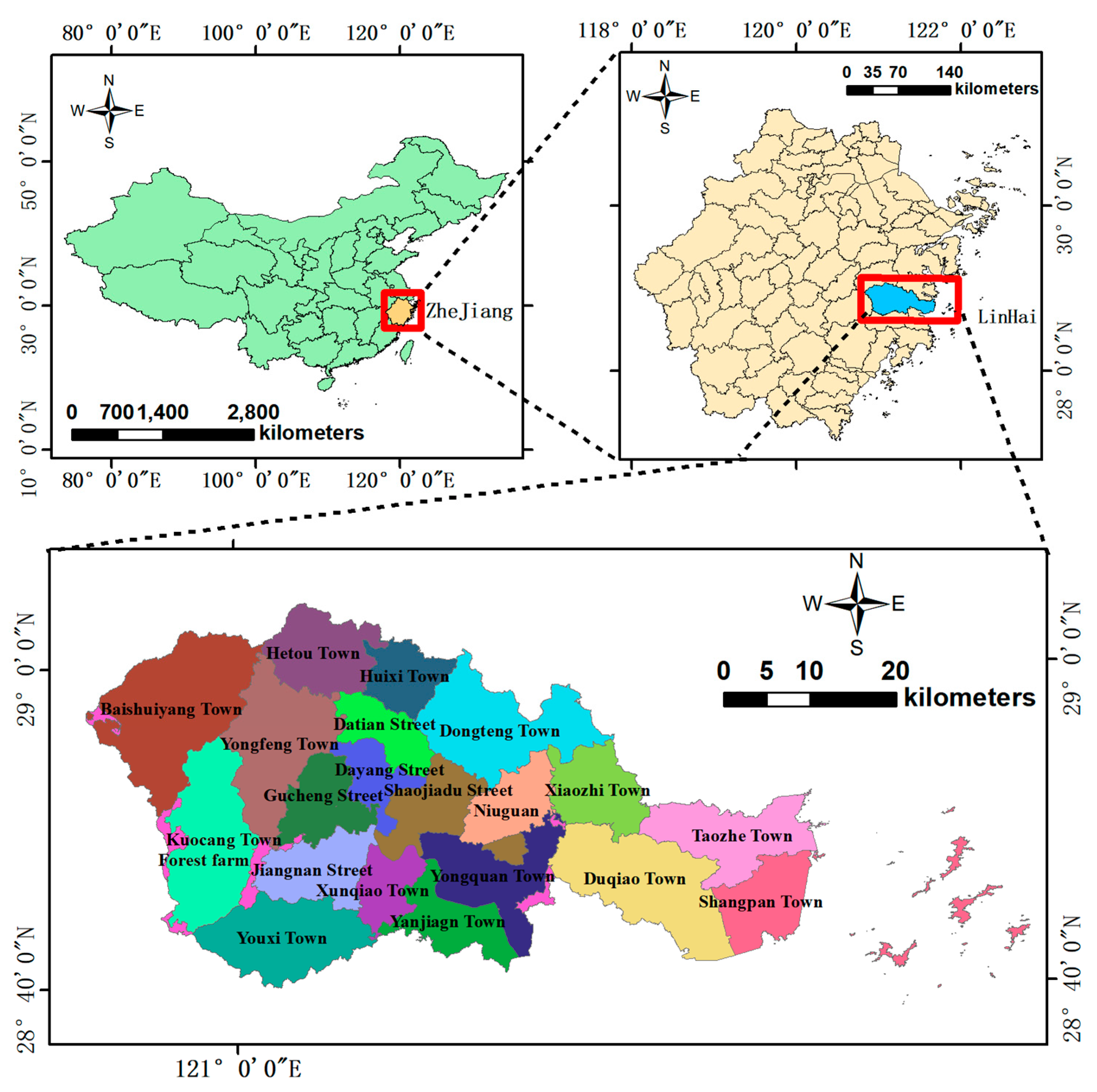
2.1. Overview of the Research Area

Linhai City (shown in Figure 1) is located on the southeast coast of Zhejiang Province, at 28°40′~29°04′ N and 120°49′~121°41′ E. The maximum distance between east and west is 85 km, and the maximum distance between north and south is 44 km. The total land area is 2203 km2. The territory is dominated by mountains and hills and has a subtropical monsoon climate. Linhai City is a key forestry county in Zhejiang Province, with a forest area of 150,396 ha, a total forest growing stock of 4,280,000 m3, and a forest coverage rate of 58.6%.

2.2. Research Data

2.2.1. Remote Sensing Data

The optical remote sensing data with four-scene images generated by the satellite Sentinel-2 on 27 November 2017 and 31 October 2017 were used in this study. The radar remote sensing data with two-scene images were generated by the satellite Sentinel-1 in October 2017. The remote sensing data were obtained from the European Space Agency (ESA) website (https://scihub.copernicus.eu/ (accessed on 15 December 2020)), and the details with specifications and dates of acquisition are shown in Table 1.
From the Sentinel-2B level 1-C product, the atmospheric correction is performed by the plug-in software of Sen2cor to eliminate the radiation errors caused by the atmosphere, and resampling is performed by SNAP software. Furthermore, ENVI software is used to convert the image coordinate system from the Global Navigation Satellite System (GNSS) to the China Geodetic Coordinate System 2000 (CGCS2000) and perform a mosaic to fuse the four-scene optical images into a complete image. Finally, based on the administrative vector map of Linhai City, the mosaic remote sensing image is cropped. Therefore, an optical remote sensing image consistent with the boundary of the study area is obtained.
The propagation and scattering of electromagnetic waves are both vector phenomena, and polarization is used to study the vector characteristics of electromagnetic waves. The radar can transmit horizontal (H) or vertical (V) electric field vectors, and can also receive horizontal (H) or vertical (V) signals. HH, VV, HV, and VH are four polarization modes commonly used in the Sentinel-1 radar remote sensing system. VV–VH is mainly used to observe land, while HH–HV and HH are usually used to monitor polar environments. The Sentinel-1 radar remote sensing image obtained in this study is a ground distance multi-view product in IW GRD interference wide mode (TOPS Mode), with rising orbit and two polarization modes of VV and VH. To eliminate or reduce the errors by noise, radiation, and terrain fluctuations from the original product, the radar remote sensing images are preprocessed by SNAP software using the following operations: thermal noise removal, radiation correction, speckle filtering, radiometric calibration, and terrain correction [9]. Furthermore, the radar remote sensing images are preprocessed by the operations of transformation of the coordinate system, mosaic, and crop.

2.2.2. Ground Data

The ground data used in this paper are DEM (Figure 2) and the inventory data for forest management planning and design in 2017.
The DEM data with 30 m resolution and the World Geodetic System 1984 (WGS84), including four-scene images, are supplied by the International Scientific & Technical Data Mirror Site, Computer Network Information Center, Chinese Academy of Sciences (www.gscloud.cn (accessed on 15 December 2020)). The preprocessing operations of transformation of the coordinate system, mosaic, and crop for the DEM images are described in Section 2.2.1.
The inventory data for forest management planning and design, containing 59,636 sub-compartments, were provided by the Forestry Bureau of Linhai in 2017. In order to eliminate erroneous and incorrect data, the following two steps are implemented: the first step is to remove the samples with non-forest, zero-volume, or zero-canopy density sub-compartments; the second step is to further remove the samples according to the principle of three times the standard deviation [43]. Finally, 18,987 valid samples were involved in the following research, including 10 dominant tree species (mixed broadleaf forest, mixed coniferous and broadleaf forest, other hard wide class, Pinus massoniana, mixed coniferous forest, Chinese fir, Camphor, Schima superba, other soft broad class, cedar). The sub-compartments ranged in size from 2000 m2 to 359,333 m2, and the distribution of the stock volume per hectare is shown in Figure 3.

2.3. Independent Variable Factor Extraction

2.3.1. The Independent Variable Factors from Optical Remote Sensing Images

The independent variables from optical remote sensing images of Sentinel-2 include two types of factors: original factors (Band 1, Band 2, Band 3, Band 4, Band 5, Band 6, Band 7, Band 8, Band 8A, Band 9, Band 10, Band 11, Band 12) and derivational factors (vegetation indices, shown in Table 2), which are calculated by the original factors.
Of the thirteen bands originating from Sentinel-2 remote sensing images, there are four (Band 2, Band 3, Band 4, and Band 8) with a higher resolution of 10 m. After combining the four bands [63], the principal component analysis (PCA) method is utilized to eliminate collinearity and calculate important principal components [64], and from the first important principal component, eight texture-independent variable factors are obtained: mean, variance, homogeneity, contrast, dissimilarity, entropy, angular second moment, and correlation.

2.3.2. The Independent Variable Factors from Radar Remote Sensing Images

From radar remote sensing images, four independent variable factors are obtained, which are the backscatter coefficient VV, VH, the polarization ratio VV/VH, and the polarization difference VV–VH.

2.3.3. The Independent Variable Factors from Ground Data

From the inventory data for forest management planning and design, there are nine independent variable factors involved in the research, which include slope direction (PO_XIANG), slope position (PO_WEI), soil thickness (TU_CENG_HD), humus thickness (FU_ZHI_HD), vegetation coverage (ZB_FGD), forest population (QUN_LUO), dominant tree species (YOU_SHI_SZ), tree age (NL), and canopy density (YU_BI_DU). In the nine independent variables, the slope direction (PO_XIANG), humus thickness (FU_ZHI_HD), forest population (QUN_LUO), and dominant tree species (YOU_SHI_SZ) are the categorical characteristic factors. Furthermore, we extract three independent variable factors of elevation (ELEVATION), slope (SLOPE), and aspect angle (ASPECT) from DEM data.

2.3.4. Data Integration

To summarize all factors from Section 2.2.1 to Section 2.2.2, there are 34 independent variable factors and four characteristic variables (Table 3). In ArcGIS 10.2 (Environmental Systems Research Institute, Redlands, CA, USA), the DEM data and remote sensing data were extracted based on each sub-compartment. For modeling and prediction, all the preprocessed data, including the inventory data for forest management planning and design, DEM data, and remote sensing images from Sentinel-2B and Sentinel-1A, were integrated into the same relational database. The remaining 18,987 samples were randomly divided into a training set and tested set according to the ratio of 7:3.

2.4. Methods

2.4.1. Gradient Boosting Decision Tree (GBDT)

GBDT [40] is an integrated machine learning (ML) algorithm that uses multiple decision trees (DTs) as basic learners. Each decision tree (DT) is not independent because the newly added DT increases the emphasis on the misclassification samples obtained by the previous DTs. The GBDT algorithm takes the residual of the previous DTs as the input of the next DT. Thereby, the added DT is used to reduce the residual so that the loss decreases following the negative gradient direction in each iteration.

2.4.2. eXtreme Gradient Boosting (XGBoost)

XGBoost [45] is an integrated ML algorithm based on GBDT. The basic idea of the XGBoost algorithm is to first establish a base classifier/regressor and then gradually add new classifiers/regressors. After each classifier/regressor is added, the value of the objective function is calculated again to continuously improve the expression effect of the model. This algorithm has strong generalization performance and can reduce over-fitting by introducing the regularization term in the objective function, which is significantly different from the GBDT.

2.4.3. Categorical Boosting (CatBoost)

CatBoost [50] is derived from “Category” and “Boosting”, and is also a kind of boosting algorithm. The CatBoost algorithm overcomes the shortcomings of the original boosting algorithm, such as data offset problems, and is used in the processing of prediction offsets and categorical features. The following improvements have been made:
  • To predict the offset: Traditional gradient enhancement depends on the sample itself for gradient calculation, and noise points will bring prediction offsets and eventually lead to overfitting. CatBoost first sorts the entire dataset several times and then removes the i-th data item for the first i-1 pieces of data, calculates the loss function and gradient, builds a residual tree, and finally adds the residual tree to the original model, which effectively avoids the prediction offset and reduces overfitting.
  • To process the category features: The CatBoost algorithm can automatically process categorical features and combine the original category features according to the inherent relationship of the features, which enriches the feature dimensions to improve the accuracy of the prediction results. In addition, the automatic processing of category features also greatly improves efficiency.
Suppose the observation dataset S = {(X1, Y1), (X2, Y2),…, (Xn, Yn)}, where Xi = (xi1, xi2,…, xin) is the n-dimensional vector of a set of numerical features and categorical features, and Yi is the labeled value.
Firstly, the CatBoost algorithm binarizes all numerical features: the oblivious tree is used as the base predictor to binarize the floating point features, statistical information, and codes by one-hot encoding. Secondly, the categorical features are transformed into digital features. The specific steps are as follows.
(1)
To randomly arrange the categorical features to generate multiple random sequences.
(2)
To replace each sequence’s value with the average label value of the training dataset (shown in Formula (1)).
x i k = j = 1 n [ x j k = = x i k ] * Y j j = 1 n [ x j k = = x i k ]
where if xjk == xik, then [xjk = xik] = 1; otherwise, xjk = 0.
(3)
To convert the sequence’s value into a numerical value (shown in Formula (2)).
x θ p , k = j = 1 p 1 [ x θ j , k = x θ p , k ] + a * P j = 1 p 1 [ x θ j , k = x θ p , k ] + a
where θ = ( θ 1 ,     θ 2 , θ n ) n T , P is the prior value, and a is the coefficient of the weight for the prior of P.
A relatively novel algorithm with very powerful prediction ability, the CatBoost model was developed in 2018, and it is worth applying to estimate forest growing stock.

2.4.4. Least Absolute Shrinkage and Selection Operator (Lasso)

Lasso [51] is an embedded feature selection method. By adding the L1 penalty term, Lasso reduces the value to 0 to the coefficients of those nonsignificant features, so as to remove them from the independent variables. Compared with other variable selection methods, the Lasso method has the advantages of higher effectiveness and better stability.

2.5. Model Performance Indicators

We chose a 10-fold cross-validation method to evaluate the accuracy of the model. The performance indicators include the coefficient of determination (R-squared, R2), mean square error (MSE), mean absolute error (MAE), mean absolute percentage error (MAPE), root mean square error (RMSE), and relative root mean square error (RMSEr), calculated by Formulas (3)–(8).
R 2 = i = 1 N ( y i   y - ) 2 i = 1 N ( y i   y - ) 2
MSE = 1 N i = 1 N ( y i y i ) 2
MAE = 1 N i = 1 N | ( y i y i ) |
MAPE = 1 N i = 1 N | ( y i y i ) | y i
RMSE = MSE
RMSE r = RMSE   y -
where N represents the number of samples, y i is the i-th measured value, y i ^ is the estimated value,   y - is the mean of all y i , and the expression for calculating   y - is   y - = 1 N i = 1 N y i .

3. Results

Based on whether to add category features and whether to add Sentinel-1 remote sensing data, four data schemes are designed: A, B, C, and D (as shown in Table 4).

3.1. Screening for Independent Variable Factors

3.1.1. Variable Screening for Data Schemes A and B

Based on data schemes A and B, which include the data sources of Sentinel-2, DEM, and inventory data for forest management planning and design, a total of 30 initial numerical features are extracted. Furthermore, the Lasso method is used to select more critical independent variable factors from the 30 numerical features. After parameter tuning for the Lasso, the value of alpha is set to 0.0005, and the value of the threshold coefficient is set to 0.02. Finally, the remaining independent variables (Figure 4a) include five factors, namely, canopy density (YU_BI_DU), correlation, tree age (NL), variance, and entropy.

3.1.2. Variable Screening for Data Schemes C and D

Based on the data schemes C and D, which include the data sources of Sentinel-2, Sentinel-1, DEM, and inventory data for forest management planning and design, a total of 34 initial numerical features are extracted. Using the same feature selection method and parameter values as in Section 3.1.1, seven independent variables (Figure 4b) remain, namely, canopy density (YU_BI_DU), polarization ratio (VV/VH), variance (VARIANCE), tree age (NL), backscatter coefficient (VV), entropy (ENTROPY), and correlation (CORRELATION).

3.2. Result Analysis

3.2.1. Analysis for Data Schemes A and B

From the data schemes A and B, with the five remaining factors of canopy density (YU_BI_DU), correlation (Correlation), tree age (NL), variance (VARIANCE), and entropy (ENTROPY) as independent variables, and the forest growing stock per hectare as the dependent variable, the models based on GBDT, XGBoost, and CatBoost are developed. The performance indicators of models to estimate the forest growing stock based on data schemes A and B are shown in Table 5.
The models based on data scheme B have four more category features than data scheme A. The performance indicators are evidently improved, with R2 increases of 9.20–11.76%. The MSE, MAE, and MAPE decrease by 17.40–26.47%, 9.20–16.20%, and from 24.70–27.02% to 21.03–24.64%, respectively. It can also be seen from the performance indicators that the CatBoost algorithm is the best model to estimate forest growing stock. In the model of CatBoost, when using data scheme A, the highest value of R2 is 0.68, and the lowest MAPE is 24.70%. When using data scheme B, the highest value of R2 is 0.76, and the lowest MAPE is 21.03%.

3.2.2. Analysis for Data Schemes C and D

The models based on data scheme D have four more category features than data scheme C. The performance indicators are also evidently improved, with R2 increases of 14.29–20.00%. The MSE, MAE, and MAPE decrease by 25.71–40.38%, 12.82–23.38%, and from 21.03–23.71% to 16.20–20.28%, respectively. It can also be seen from the performance indicators that the CatBoost algorithm is the best model to estimate forest growing stock. In the model of CatBoost, when using data scheme C, the highest value of R2 is 0.65, and the lowest MAPE is 21.63%. When using data scheme D, the highest value of R2 is 0.78, and the lowest MAPE is 16.20%. Furthermore, comparing scheme C with scheme A, there is only a slight gap for the three indicators of R2, MSE, and MAE. However, the MAPE significantly decreased by 11.96–12.43% for the models XGBoost, GBDT, and CatBoost. The comparative study of scheme D and scheme B also shows that the MAPE significantly decreased by 17.70–22.97% for the models GBDT, XGBoost, and CatBoost.
Figure 5 depicts a comprehensive and intuitive comparison of the performance indicators generated by the models GBDT, XGBoost, and CatBoost, showing that CatBoost is the best model to estimate forest growing stock. Regarding the data sources, data scheme D is the best scheme. The introduction of category features effectively improves the performance, and the radar remote sensing factors can also be used to improve the estimation accuracy with a significant decrease in the MAPE.
In detail, Figure 6 shows a scatter plot of the estimated values (values calculated by models) and measured values (values from the inventory data) for the sub-compartments based on the four data schemes (schemes A, B, C, and D) and the three models (GBDT, XGBoost, and CatBoost). It has been experimentally proven that the performance indicators of R2 and MAPE with category features (in data schemes B and D) are significantly better than those without category features (in data schemes A and C). Furthermore, the introduction of radar remote sensing factors efficiently reduces the MAPE so that a higher accuracy can be obtained for estimating forest growing stock. Additionally, the scattered points generated by CatBoost are closer to sub-diagonal (the diagonal from bottom left to top right) than the ones generated by GBDT and XGBoost.

4. Discussion

4.1. Principal Findings

From the research results, we can make the following points. (1) The Lasso feature selection method can effectively remove non-significant indicators. (2) Compared with other machine learning models, the CatBoost model has obvious advantages in estimating the forest growing stock. (3) The addition of category features significantly improves the performance of the models.

4.2. Comparison with Other Studies

Among the performance indicators, R2 represents the fitting degree between the measured values and estimated values, and RMSEr (%) and MAPE (%) represent the model’s estimated deviation degree of the measured values. Because the three indicators reflect the relative relationship between measured data and estimated data rather than absolute deviation, they can avoid being affected by the measurement unit of sample data, so they are more suitable for performance comparison between different studies. Accordingly, we compared our study with existing relevant studies in the performance indicators of R2, RMSEr (%), and MAPE (%) (shown in Table 6).
Table 6 shows that the performance indicators of RMSEr (%) and MAPE (%) in our study are significantly improved compared with previous studies [43,65,66]; the R2 is also maintained at a relatively higher level than in the research by Mauya (2019) and Ruyi Zhou (2018).
The estimation accuracy of this study is 83.8%, which is slightly lower than the 84.5% estimation accuracy of Huang Yuling et al. [67], who used only 4002 experimental samples, which is far lower than our study with 18,987 data samples. The R2 in this study is 0.78, which is less than 0.84, the value of R2 in the study by Jingjing Zhou (2020). While comparing the study area between our study and that of Jingjing Zhou, an indisputable fact is that the former is 150,396 ha, which is much larger than the latter’s 7600 ha. This shows that the CatBoost algorithm used in this study has relatively high accuracy and generalization ability to estimate forest growing stock, even in the case of a larger amount of data and larger study area size than previous studies.

4.3. Strengths and Limitations of This Study

We utilized multi-source data, which include the optical remote sensing data from the satellite of Sentinel-2, radar remote sensing data from the satellite of Sentinel-1, DEM, and inventory data for forest management planning and design. An initial independent variable set is established, which includes spectral features from Sentinel-2, texture features from Sentinel-2, polarization features from Sentinel-1, topographic features (elevation, slope, and aspect angle) from DEM, and ground factors from the inventory data for forest management planning and design. Based on whether to add category features and whether to add Sentinel-1 remote sensing data, we designed four data schemes: A, B, C, and D. Additionally, the Lasso algorithm was used to select relatively important features from the initial independent variables. Finally, three models, GBDT, XGBoost, and CatBoost, were involved in the study. The main contributions are as follows:
(1)
A total of 34 independent variable factors are obtained, and the Lasso algorithm effectively reduces the number of independently variable factors so as to speed up the training process of the model and improve the generalization ability of the model.
(2)
The addition of category features significantly improves the performance of the models. This mainly depends on contributions of two aspects. One is the category features of forest population and dominant species; the addition of these category features gives more targeted estimation results according to different categories. The other is for the category features of humus thickness and aspect direction; the addition of these category features further reflects the relationship between the plant growth and the environmental factors, e.g., plants with thicker humus or on sunny slopes tend to grow better. Therefore, the model inclines to obtain a higher accuracy after adding category features.
(3)
It is easier to obtain the vertical structure parameters of vegetation by radar remote sensing data, which can overcome the shortcomings of optical remote sensing data to a certain extent. Thus, the combination of radar remote sensing data and optical remote sensing data can be used to estimate forest growing stock more accurately than single remote sensing data.
(4)
When adding the radar remote sensing data and the category features, the performance of the model improved significantly. Compared with data scheme A (without radar remote sensing data and without category features), for scheme D (with radar remote sensing data and with category features), the R2 increased by 10.76–14.71%, while MSE, MAE, and MAPE decreased by 28.44–39.22%, 10.53–20.27%, and from 24.70–27.02% to 16.20–20.28%, respectively.
(5)
CatBoost first sorts the entire dataset several times and then removes the i-th data item, and builds residual trees and adds them to the original model step by step, which effectively avoids the prediction offset and reduces overfitting. Furthermore, the CatBoost algorithm can automatically process categorical features and combines the original category features according to the inherent relationship of the features, which enriches the feature dimensions to improve the accuracy of the prediction results. Thus, CatBoost is the best of the three models GBDT, XGBoost, and CatBoost. When based on data scheme D, the performance indicators of the CatBoost model are R2 of 0.78, MSE of 0.62 m3/ha, MAE of 0.59 m3/ha, and MAPE of 16.20%. Moreover, the estimation accuracy is close to 85%, which has practical significance and benefit in estimating the forest growing stock.
Different from existing studies, we performed label encoding and one-hot encoding on category features and applied them to model estimation. In addition, we also attempted to use the CatBoost model to estimate large-scale forest growing stock. This is also the main innovation of this paper.
However, due to the limitations of experimental conditions, the following points need to be optimized and improved:
(1)
The texture features of remote sensing images can effectively improve the estimation accuracy to estimate forest growing stock. However, we only extracted the texture features from optical remote sensing images. If various window sizes, asynchronous lengths, and combinations from various bands are used to extract the texture features of radar remote sensing images, it would be helpful to explore the impact of texture features to improve the estimating accuracy [11].
(2)
The imaging date of remote sensing images used in this study is between October and November. There are some inconsistencies with the tree growth period. In the autumn and winter, some tree species are entering dormancy, which may lead to yellowing and even falling leaves. The vegetation information reflected from the remote sensing images, especially the optical remote sensing images, may not correctly reflect the sincere information of trees, which would reduce the estimation accuracy of the models. If remote sensing images with an imaging date consistent with the growth period of trees can be found in the future, the estimating accuracy may be further optimized.
(3)
It is necessary to verify the generality of the model through a more extensive range of the estimation of forest growing stock volume. Santoro et al. [68]’s research on global biomass estimates will provide us with a validation set.

5. Conclusions

In this study, optical remote sensing data, radar remote sensing data, DEM data, and inventory data for forest management planning and design were used to estimate the forest growing stock of 18,987 sub-compartments in Linhai City using three machine learning algorithms. Our specific conclusions are as follows:
(1)
The Lasso algorithm effectively reduced the number of independent variable factors and retained the main features, speeding up the training process of the model and improving the generalization ability of the model.
(2)
Radar remote sensing waves more easily penetrate the forest surface to obtain the vertical parameters of the forest, which makes up for the shortcomings of optical remote sensing data sources to a certain extent and could improve the estimation accuracy of forest growing stock.
(3)
The addition of category features led to more targeted estimation and significantly improved the performance of the models.
(4)
To estimate the forest growing stock, the CatBoost algorithm is the best model among the three models GBDT, XGBoost, and CatBoost. Distinguished from the common artificial classification methods which established different models according to various category characteristics, the CatBoost model is more efficient and convenient.

Author Contributions

Conceptualization, D.W.; Formal analysis, D.W.; Funding acquisition, L.F.; Methodology, X.Z.; Resources, L.F.; Writing—original draft, H.H. All authors have read and agreed to the published version of the manuscript.

Funding

This work was financially supported by the Zhejiang Provincial Key Science and Technology Project (2018C02013).

Data Availability Statement

Remote sensing data can be found here: [https://scihub.copernicus.eu/], accessed on 3 August 2022. DEM data can be found here: [www.gscloud.cn], accessed on 3 August 2022. The ground survey data are not publicly available due to [For policy reasons, this data is kept confidential].

Conflicts of Interest

The authors declare no conflict of interest.

References

  1. Lu, D.; Chen, Q.; Wang, G. A survey of remote sensing-based aboveground biomass estimation methods in forest ecosystems. Int. J. Digit. Earth. 2014, 9, 63–105. [Google Scholar] [CrossRef]
  2. Scrinzi, G.; Marzullo, L.; Galvagni, D. Development of a neural network model to update forest distribution data for managed alpine stands. Ecol. Model. 2007, 206, 331–346. [Google Scholar] [CrossRef]
  3. Santoro, M.; Cartus, O.; Fransson, J. Estimates of forest growing stock for Sweden, Central Siberia, and Québec Using Envisat Advanced Synthetic Aperture Radar Backscatter Data. Remote Sens. 2013, 5, 4503–4532. [Google Scholar] [CrossRef]
  4. Tanaka, S.; Takahashi, T.; Nishizono, T. Stand Volume Estimation Using the k-NN Technique Combined with Forest Inventory Data, Satellite Image Data and Additional Feature Variables. Remote Sens. 2015, 7, 378–394. [Google Scholar] [CrossRef]
  5. Mohammadi, Z.; Mohammadi Limaei, S.; Lohmander, P. Estimation of a basal area growth model for individual trees in uneven-aged Caspian mixed species forests. J. For. Res. 2017, 29, 1205–1214. [Google Scholar] [CrossRef]
  6. Wu, D.; Ji, Y. Dynamic Estimation of Forest Volume Based on Multi-Source Data and Neural Network Model. J. Agric. Sci. 2015, 7, 18. [Google Scholar] [CrossRef]
  7. Maselli, F.; Chiesi, M.; Mura, M. Combination of optical and LiDAR satellite imagery with forest inventory data to improve wall-to-wall assessment of growing stock in Italy. Int. J. Appl. Earth Obs. Geoinf. 2014, 26, 377–386. [Google Scholar] [CrossRef]
  8. Chirici, G.; Barbati, A.; Corona, P. Non-parametric and parametric methods using satellite images for estimating growing stock volume in alpine and Mediterranean forest ecosystems. Remote Sens. Environ. 2008, 112, 2686–2700. [Google Scholar] [CrossRef]
  9. Tomppo, E.; Halme, M. Using coarse scale forest variables as ancillary information and weighting of variables in k-NN estimation: A genetic algorithm approach. Remote Sens Environ. 2004, 92, 1–20. [Google Scholar] [CrossRef]
  10. Boisvenue, C.; Smiley, B.P.; White, J.C. Integration of Landsat time series and field plots for forest productivity estimates in decision support models. For. Ecol. Manag. 2016, 376, 284–297. [Google Scholar] [CrossRef]
  11. Wang, K.N.; Lv, J.; Li, C.G. Inversion of Growing Stock Volume Using Satellite Image Multiscale Texture Feature. J. Cent. South Univ. 2017, 37, 84–89. (In Chinese) [Google Scholar]
  12. Hao, L.; Liu, H.; Chen, Y.F. Remote Sensing Estimation of forest growing stock Based on Spectral and Texture Information. J. Mt. Sci. 2017, 35, 246–254. (In Chinese) [Google Scholar]
  13. Chrysafis, I.; Mallinis, G.; Siachalou, S. Assessing the relationships between growing stock volume and Sentinel-2 imagery in a Mediterranean forest ecosystem. Remote Sens. Lett. 2017, 8, 508–517. [Google Scholar] [CrossRef]
  14. Sothe, C.; Almeida, C.; Liesenberg, V. Evaluating Sentinel-2 and Landsat-8 Data to Map Successional Forest Stages in a Subtropical Forest in Southern Brazil. Remote Sens. 2017, 9, 838. [Google Scholar] [CrossRef]
  15. Mura, M.; Bottalico, F.; Giannetti, F. Exploiting the capabilities of the Sentinel-2 multi spectral instrument for predicting growing stock volume in forest ecosystems. Int. J. Appl. Earth Obs. Geoinf. 2018, 66, 126–134. [Google Scholar] [CrossRef]
  16. Wang, Z.M.; Yue, C.Y.; Liu, Q. Study on Model of Forest Volume Estimation Based on Optical and Microwave Remote Sensing Data. Southwest China J. Agric. Sci. 2018, 31, 1722–1726. (In Chinese) [Google Scholar]
  17. Chowdhury, T.A.; Thiel, C.; Schmullius, C. Growing stock volume estimation from L-band ALOS PALSAR polarimetric coherence in Siberian forest. Remote Sens. Environ. 2014, 155, 129–144. [Google Scholar] [CrossRef]
  18. Thiel, C.; Schmullius, C. The potential of ALOS PALSAR backscatter and InSAR coherence for forest growing stock estimation in Central Siberia. Remote Sens. Environ. 2016, 173, 258–273. [Google Scholar] [CrossRef]
  19. Yang, M.S.; Xu, T.S.; Niu, X.H. Estimation of Pinus Kesiya var. Langbianensis Forest Stock Volume Based on Sentinel-1A SAR Image. J. West China For. Sci. 2019, 48, 52–58. (In Chinese) [Google Scholar]
  20. Laurin, G.V.; Balling, J.; Corona, P. Above-ground biomass prediction by Sentinel-1 multitemporal data in central Italy with integration of ALOS2 and Sentinel-2 data. J. Appl. Remote Sens. 2018, 12, 016008. [Google Scholar] [CrossRef]
  21. Ningthoujam, R.; Balzter, H.; Tansey, K.; Morrison, K.; Johnson, S.; Gerard, F.; George, C.; Malhi, Y.; Burbidge, G.; Doody, S.; et al. Airborne S-Band SAR for Forest Biophysical Retrieval in Temperate Mixed Forests of the UK. Remote Sens. 2016, 8, 609. [Google Scholar] [CrossRef]
  22. Du, J.; Shi, J.; Sun, R. The development of HJ SAR soil moisture retrieval algorithm. Int. J. Remote Sens. 2010, 31, 3691–3705. [Google Scholar] [CrossRef]
  23. Bird, R.; Whittaker, P.; Stern, B.; Angli, N.; Cohen, M.; Guida, R. NovaSAR-S a low cost approach to sar applications, synthetic aperture radar. In Proceedings of the IEEE 2013 Asia-Pacific Conference on Synthetic Aperture Radar (APSAR), Tsukuba, Japan, 23–27 September 2013; pp. 84–87. [Google Scholar]
  24. Jet Propulsion Laboratory (JPL). Mission to Earth: NASA-ISRO Synthetic Aperture Radar. Available online: http://www.Jpl.Nasa.Gov/missions/nasa-isro-synthetic-aperture-radar-nisar/ (accessed on 15 December 2015).
  25. Jet Propulsion Laboratory (JPL). Overview. Available online: https://nisar.jpl.nasa.gov/mission/get-to-know-sar/overview/ (accessed on 4 September 2022).
  26. Torbick, N.; Ledoux, L.; Salas, W. Regional Mapping of Plantation Extent Using Multisensor Imagery. Remote Sens. 2016, 8, 236. [Google Scholar] [CrossRef]
  27. Shao, Z.; Zhang, L. Estimating Forest Aboveground Biomass by Combining Optical and SAR Data: A Case Study in Genhe, Inner Mongolia, China. Sensors 2016, 16, 834. [Google Scholar] [CrossRef] [Green Version]
  28. Zhao, P.; Lu, D.; Wang, G. Forest aboveground biomass estimation in Zhejiang Province using the integration of Landsat TM and ALOS PALSAR data. Int. J. Appl. Earth Obs. Geoinf. 2016, 53, 1–15. [Google Scholar] [CrossRef]
  29. Fedrigo, M.; Meir, P.; Sheil, D. Fusing radar and optical remote sensing for biomass prediction in mountainous tropical forests. In Proceedings of the 2013 IEEE International Geoscience and Remote Sensing Symposium, IGARSS, Melbourne, Australia, 21–26 July 2013. [Google Scholar]
  30. Vafaei, S.; Soosani, J.; Adeli, K. Improving Accuracy Estimation of Forest Aboveground Biomass Based on Incorporation of ALOS-2 PALSAR-2 and Sentinel-2A Imagery and Machine Learning: A Case Study of the Hyrcanian Forest Area (Iran). Remote Sens. 2018, 10, 172. [Google Scholar] [CrossRef]
  31. Chirici, G.; Giannetti, F.; Mcroberts, R.E. Wall-to-wall spatial prediction of growing stock volume based on Italian National Forest Inventory plots and remotely sensed data. Int. J. Appl. Earth Obs. Geoinf. 2020, 84, 101959. [Google Scholar] [CrossRef]
  32. Lu, D.; Batistella, M.; Li, G. Land use/cover classification in the Brazilian Amazon using satellite images. Pesqui. Agropecu. Bras. 2012, 47. [Google Scholar] [CrossRef]
  33. Drusch, M.; Bello, U.D.; Carlier, S. Sentinel-2: ESA’s Optical High-Resolution Mission for GMES Operational Services. Remote Sens. Environ. 2012, 120, 25–36. [Google Scholar] [CrossRef]
  34. Puliti, S.; Saarela, S.; Gobakken, T. Combining UAV and Sentinel-2 auxiliary data for forest growing stock estimation through hierarchical model-based inference. Remote Sens. Environ. 2018, 204, 485–497. [Google Scholar] [CrossRef]
  35. Zharko, V.O.; Bartalev, S.A.; Sidorenkov, V.M. Forest growing stock estimation using optical remote sensing over snow-covered ground: A case study for Sentinel-2 data and the Russian Southern Taiga region. Remote Sens. Lett. 2020, 11, 677–686. [Google Scholar] [CrossRef]
  36. Macintyre, P.; Niekerk, A.; Mucina, L. Efficacy of multi-season Sentinel-2 imagery for compositional vegetation classification. Int. J. Appl. Earth Obs. Geoinf. 2020, 85, 101980. [Google Scholar] [CrossRef]
  37. Grabska, E.; Hostert, P.; Pflugmacher, D. Forest Stand Species Mapping Using the Sentinel-2 Time Series. Remote Sens. 2019, 11, 1197. [Google Scholar] [CrossRef]
  38. Reis, M.S.; Dutra, L.V.; Sant’Anna, S.J.S. Multi-source change detection with PALSAR data in the Southern of Pará state in the Brazilian Amazon. Int. J. Appl. Earth Obs. Geoinf. 2020, 84, 101945. [Google Scholar] [CrossRef]
  39. Rumora, L.; Miler, M.; Medak, D. Impact of Various Atmospheric Corrections on Sentinel-2 Land Cover Classification Accuracy Using Machine Learning Classifiers. ISPRS Int. J. Geo-Inf. 2020, 9, 277. [Google Scholar] [CrossRef]
  40. Were, K.; Bui, D.T.; Dick, Ø.B.; Singh, B.R. A comparative assessment of support vector regression, artificial neural networks, and random forests for predicting and mapping soil organic carbon stocks across an Afromontane landscape. Ecol. Indic. 2015, 52, 394–403. [Google Scholar] [CrossRef]
  41. Dos Reis, A.A.; Carvalho, M.C.; Mello, J.M. Spatial prediction of basal area and volume in Eucalyptus stands using Landsat TM data: An assessment of prediction methods. N. Z. J. For. Sci. 2018, 48, 1. [Google Scholar] [CrossRef]
  42. Esteban, J.; Mcroberts, R.; Fernández-Landa, A. Estimating Forest Volume and Biomass and Their Changes Using Random Forests and Remotely Sensed Data. Remote Sens. 2019, 11, 1944. [Google Scholar] [CrossRef]
  43. Zhou, R.Y.; Wu, D.S.; Fang, L.M. A Levenberg-Marquardt Backpropagation Neural Network for Predicting Forest Growing Stock Based on the Least-Squares Equation Fitting Parameters. Forests 2018, 9, 757. [Google Scholar] [CrossRef]
  44. Friedman, J.H. Greedy Function Approximation: A Gradient Boosting Machine. Ann. Stat. 2001, 29, 1189–1232. [Google Scholar] [CrossRef]
  45. Chen, T.; Guestrin, C. XGBoost: A Scalable Tree Boosting System. In Proceedings of the 22Nd ACM SIGKDD International Conference on Knowledge Discovery and Data Mining, San Francisco, CA, USA, 13–17 August 2016; pp. 785–794. [Google Scholar]
  46. Yu, D.; Liu, Z.; Su, C. Copy number variation in plasma as a tool for lung cancer prediction using Extreme Gradient Boosting (XGBoost) classifier. Thorac. Cancer 2020, 11, 95–102. [Google Scholar] [CrossRef] [PubMed]
  47. Liang, W.; Luo, S.; Zhao, G. Predicting Hard Rock Pillar Stability Using GBDT, XGBoost, and LightGBM Algorithms. Mathematics 2020, 8, 765. [Google Scholar] [CrossRef]
  48. Liu, T.; Jiang, T.; Ang, L.I.; Guo, L. Remote sensing estimation of forest stock volume based on neural network and different site quality. J. Shandong Univ. Sci. Technol. Sci. 2019, 38, 25–35. (In Chinese) [Google Scholar] [CrossRef]
  49. Wang, Z.; Xu., T.S.; Yue, C.R. Application of Dummy Variable in the Research of Pinus densata Stock Volume Inversion Model. For. Resour. Manag. 2017, 75–81. (In Chinese) [Google Scholar] [CrossRef]
  50. Dorogush, A.V.; Ershov, V.; Gulin, A. CatBoost: Gradient boosting with categorical features support. arXiv 2018, arXiv:1810.11363. [Google Scholar]
  51. Tibshirani, R. Regression Shrinkage and Selection Via the Lasso. J. R. Stat. Soc. Ser. B Methodol. 1996, 58, 267–288. [Google Scholar] [CrossRef]
  52. Huete, A.R. A soil-adjusted vegetation index (SAVI). Remote Sens. Environ. 1988, 25, 295–309. [Google Scholar] [CrossRef]
  53. Jordan, C.F. Derivation of Leaf-Area Index from Quality of Light on the Forest Floor. Ecology 1969, 50, 663–666. [Google Scholar] [CrossRef]
  54. Goel, N.S.; Qin, W. Influences of canopy architecture on relationships between various vegetation indices and LAI and Fpar: A computer simulation. Remote Sens. Rev. 1994, 10, 309–347. [Google Scholar] [CrossRef]
  55. Rouse, J.W., Jr.; Hass, R.H. Monitoring Vegetation Systems in the Great Plains with ERTS; Texas A&M University: College Station, TX, USA, 1974; Volume 20, pp. 309–313. [Google Scholar]
  56. Sims, D.A.; Gamon, J.A. Relationships between leaf pigment content and spectral reflectance across a wide range of species, leaf structures and developmental stages. Remote Sens. Environ. 2002, 81, 337–354. [Google Scholar] [CrossRef]
  57. Hardisky, M.S.; Klemas, V. The influence of soil salinity, growth form, and leaf moisture on the spectral radiance of Spartina Alterniflora canopies. Photogramm. Eng. Remote Sens. 1983, 49, 77–84. [Google Scholar]
  58. Yang, W.; Kobayashi, H.; Wang, C.; Shen, M.G.; Chen, J.; Matsushita, B.; Tang, Y.H.; Kim, Y.W.; Bret-Harte, S.; Zona, D.; et al. A semi-analytical snow-free vegetation index for improving estimation of plant phenology in tundra and grassland ecosystems. Remote Sens. Environ. 2019, 228, 31–44. [Google Scholar] [CrossRef]
  59. Huete, A.R.; Liu, H.Q.; Batchily, K.; YanLeeuwen, W. A comparison of vegetation indices global set of TM images for EOS-MODIS. Remote Sens. Environ. 1997, 59, 440–451. [Google Scholar] [CrossRef]
  60. Richardson, A.J.; Wiegand, C.L. Distinguishing vegetation from soil background information. Photogramm. Eng. Remote Sens. 1977, 43, 1541–1552. [Google Scholar]
  61. Cao, L. Estimation of Forest Stock Volume in Yuqing District Based on Sentinel-2 Image. Master’s Thesis, Beijing Forestry University, Beijing, China, 2019. (In Chinese). [Google Scholar]
  62. Gitelson, A.A.; Merzlyak, M.N. Remote estimation of chlorophyll content in higher plant leaves. Int. J. Remote Sens. 1997, 18, 2691–2697. [Google Scholar] [CrossRef]
  63. Cao, L.; Peng, D.L.; Wang, X.J. Estimation of Forest Stock Volume with Spectral and Textural Information from the Sentinel-2A. J. Northeast For. Univ. 2018, 46, 54–58. (In Chinese) [Google Scholar]
  64. Liu, M.Y.; Wang, X.L.; Feng, Z.K. Estimation of Laotudingzi Nature Reserve Forest Volume Based on Principal Component Analysis. J. Cent. South Univ. 2017, 37, 80–83. (In Chinese) [Google Scholar]
  65. Mauya, E.W.; Koskinen, J.; Tegel, K. Modelling and Predicting the Growing Stock Volume in Small-Scale Plantation Forests of Tanzania Using Multi-Sensor Image Synergy. Forests 2019, 10, 279. [Google Scholar] [CrossRef]
  66. Zhou, J.; Zhou, Z.; Zhao, Q. Evaluation of Different Algorithms for Estimating the Growing Stock Volume of Pinus massoniana Plantations Using Spectral and Spatial Information from a SPOT6 Image. Forests 2020, 11, 540. [Google Scholar] [CrossRef]
  67. Huang, Y.L.; Wu, D.S.; Fang, L.M. Forest stock volume estimation based on XGboost method of stepwise regression. J. Cent. South Univ. For. Technol. 2020, 40, 72–80. (In Chinese) [Google Scholar]
  68. Santoro, M.; Cartus, O.; Carvalhais, N.; Rozendaal, D.M.A.; Avitabile, V.; Araza, A.; de Bruin, S.; Herold, M.; Quegan, S.; Rodríguez-Veiga, P.; et al. The Global Forest Above-Ground Biomass Pool for 2010 Estimated from High-Resolution Satellite Observations. Earth Syst. Sci. Data 2021, 13, 3927–3950. [Google Scholar] [CrossRef]
Figure 1. Administrative map of the study area.
Forests 13 01471 g001
Figure 2. DEM image of Lin Hai for generation of terrain factors.
Forests 13 01471 g002
Figure 3. Distribution map of forest growing stock per hectare of the sample plots.
Forests 13 01471 g003
Figure 4. Importance of the independent variables calculated by Lasso.
Forests 13 01471 g004
Figure 5. Comparison of performance indicators generated by the models GBDT, XGBoost, and CatBoost based on data schemes A, B, C, and D. (a) R-squared; (b) mean square error; (c) mean absolute error; (d) mean absolute percentage error. A—Without category features, with single remote sensing data. B—With category features, with single remote sensing data. C—Without category features, with multi-source remote sensing data. D—With category features, with multi-source remote sensing data.
Forests 13 01471 g005aForests 13 01471 g005b
Figure 6. Scatter plot between the estimated values and measured values of forest growing stock based on models GBDT, XGBoost, and CatBoost. (a) Without category features, with single remote sensing data; (a1) GBDT, (a2) XGBoost, (a3) CatBoost. (b) With category features, with single remote sensing data; (b1) GBDT, (b2) XGBoost, (b3) CatBoost. (c) Without category features, with multi-source remote sensing data; (c1) GBDT, (c2) XGBoost, (c3) CatBoost. (d) With category features, with multi-source remote sensing data; (d1) GBDT, (d2) XGBoost, (d3) CatBoost.
Forests 13 01471 g006aForests 13 01471 g006b
Table 1. Details of the remote sensing data with specifications and dates of acquisition.
Type of Remote Sensing ImagesSatelliteDate of AcquisitionProduct Level
Optical remote sensingSentiniel-2B, Sentinel-2A27 November 2017, 3 scenes October 2017, 1 sceneL1C
Radar remote sensingSentinel-1A13 October 2017, 2 scenesIW GRD
Table 2. Vegetation index formulas.
No.Vegetation IndexFormulaReference
1Soil Adjusted Vegetation Index (SAVI)SAVI = ((NIR − R)/(NIR + R + L)) × 1.5[52]
2Ratio Vegetation Index (RVI)RVI = NIR/R[53]
3Nonlinear Index (NLI)NLI = ((NIR × NIR) − R)/((NIR × NIR) + R)[54]
4Normalized Difference Vegetation Index (NDVI)NDVI = (NIR − R)/(NIR + R)[55]
5Modified Normalized Difference Vegetation Index (mNDVI)mNDVI = (NIR − R)/(NIR + R − 2 × B)[56]
6Normalized Difference Infrared Index (NDII)NDII = (NIR − SWIR1)/(NIR + SWIR1)[57]
7Normalized Difference Green Index (NDGI)NDGI = (G − R)/(G + R)[58]
8Enhanced Vegetation Index (EVI)EVI = 2.5 × (NIR − R)/(NIR + 6 × R − 7.5 × B + 1)[59]
9Difference Vegetation Index (DVI)DVI = NIR − R[60]
10RedEdge Ratio Vegetation Index (RVIre)RVIre = NIR/Re[61]
11RedEdge1 Normalized Difference Vegetation Index (NDVIre1)NDVIre1 = (NIR − Re1)/(NIR + Re1)[62]
12RedEdge2 Normalized Difference Vegetation Index (NDVIre2)NDVIre2 = (NIR − Re2)/(NIR + Re2)[62]
13Modified RedEdge Normalized Difference Vegetation Index (mNDVIre)mNDVIre = (NIR − Re1)/(NIR + Re1-2 × B)[56]
14RedEdge Nonlinear index(NLIre)NLIre = ((NIR × NIR) − Re1)/((NIR × NIR) + Re1)[61]
Note: L = 0.5 in most conditions; R, red; G, green; B, blue; NIR, near-infrared; SWIR, short-wave infrared; Re, RedEdge.
Table 3. List of the characteristic factors.
No.Factor NameExplanationSource of DataTypes of Factors
1–14Refer to Table 2Vegetation indexes from optical remote sensing imagesIndependent Variable Factors
15MeanMeanTexture features from optical remote sensing images
16VarianceVariance
17HomogeneityHomogeneity
18ContrastContrast
19DissimilarityDissimilarity
20EntropyEntropy
21Angular second momentAngular second moment
22CorrelationCorrelation
23VVVV polarizationRadar remote sensing images
24VHVH polarization
25VV/VHPolarization coefficient ratio
26VV-VHPolarization coefficient difference
27ELEVATIONAltitudeDigital elevation model
28SLOPESlope
29ASPECTAspect angle
30PO_WEISlope positionInventory data for forest management planning and design
31TU_CENG_HDSoil thickness
32ZB_FGDVegetation coverage
33NLTree age
34YU_BI_DUCanopy density
35QUN_LUOForest populationInventory data for forest management planning and designCategory features
36YOU_SHI_SZDominant species
37FU_ZHI_HDHumus thickness
38PO_XIANGAspect direction
Table 4. Data schemes.
Data SchemeData SourceCategory Features
ASentinel-2, DEM, Inventory data for forest management planning and designDid not add
BAdded
CSentinel-2, Sentiniel-1, DEM, Inventory data for forest management planning and designDid not add
DAdded
Table 5. Performance indicators for forest growing stock estimation based on data schemes A, B, C, and D.
Data SchemeABCD
GBDTR20.650.710.630.72
MSE1.090.901.050.78
MAE (m3/ha)0.760.690.780.68
MAPE (%)27.0224.6423.7120.28
RMSE1.040.951.020.88
RMSEr (%)25.9023.5325.4221.91
XGBoostR20.660.730.630.75
MSE1.060.861.030.71
MAE(m3/ha)0.740.660.760.62
MAPE (%)25.9322.9922.8318.28
RMSE1.030.931.010.84
RMSEr (%)25.5423.0025.1720.90
CatBoostR20.680.760.650.78
MSE1.020.751.040.62
MAE (m3/ha)0.740.620.770.59
MAPE (%)24.7021.0321.6316.20
RMSE1.010.871.020.79
RMSEr (%)25.0521.4825.2919.53
Table 6. Comparison analysis.
SchemeMauya [65]Ruyi Zhou [43]Jingjing Zhou [66]Our Study
R20.630.650.840.78
RMSEr (%)42.03%-28.77%19.53%
MAPE (%)-32.89%-16.20%
Publisher’s Note: MDPI stays neutral with regard to jurisdictional claims in published maps and institutional affiliations.

