Modeling Number of Trees per Hectare Dynamics for Uneven-Aged, Mixed-Species Stands Using the Copula Approach

Abstract

For the monitoring and management of forest resources, the main index is the stand volume, which is determined on the basis of the tree diameter, height, and number of trees per hectare of three-dimensional distribution. The development of trees in the forest stand is dynamic and is driven by random phenomena. In this study, the tree diameter, the potentially available area, and the height are described by the mixed-effect parameters of the Gompertz-type diffusion process. A normal copula function is used to connect a three-dimensional distribution to its one-dimensional margins. The newly developed model was illustrated using empirical data from 53 permanent experimental plots (measured for seven cycles), which were characterized as follows: pine forests (Pinus sylvestris), 63.8%; spruce (Picea abies), 30.2%; silver birch (Betula pendula Roth and Betula pubescens Ehrh.), 5.8%; and others, 0.2%. An analysis of the tree diameter and height of growth, including current and mean increments and inflection points, is presented. The models for the change in the number of trees per hectare with age are presented on the basis of the probabilistic density functions of the solutions of stochastic differential equations and the copula function. The dynamics of the number of trees per hectare are visualized graphically, and the goodness of fit of the newly developed models is evaluated using standard statistical measures.

1. Introduction

1.1. Background

Most often, tree species in the forest develop from generation to generation. The progressive changes in the size, shape, and function of the trees in a stand during their lifetimes, which transform the stand’s genetic potential into a living mature stand, define the dynamism of the stand and are referred to as stand growth. The development of trees in a forest stand can be understood as the interrelationship of the different tree sizes, which allows a particular tree to overcome the chaotic behavior of nature and proves that the stand exists as an integrated system, where changes in one tree size ultimately cause a corresponding change in the size of another. Trees in a forest stand do not live in isolation, as they are shaped in accordance with their interactions with their environment. The growth equation mathematically combines the two dependent variables of age and size to explain the continuous process of the two hidden forces of body expansion and size limitation [1]. As the size of a tree is determined by several components (for example, diameter, height, crown width, etc.), there exists a specific relationship between these size components during the entire growth process. Therefore, it is appropriate to expand the interpretation of the growth process of a particular size component by additionally introducing other size components and clarifying the extent of the dependencies between the response and the explanatory variables [2,3].

1.2. Research Motivation

Complex forest systems are characterized by important data features, such as dynamism, uncertainty, stochasticity, deviation of variables from the normal distribution, multicollinearity, and false correlations, which complicate the modeling and prediction of these systems. An approach is required that, under the conditions of the described data features, is able to adequately identify the processes in such systems, ensuring a high level of accuracy and efficiency. To assess the level of productivity of forest stands and to formalize their dynamics, it is appropriate to determine the link between the main components of the stand size, namely the number of trees per hectare, the average diameter of the trees at breast height (or average square diameter), and the average height of the trees using univariate or multivariate diffusion process models. The growth processes of forest stands evolve under the influence of random noise, which is mostly expressed by Brownian motion. Traditionally, special types of stochastic differential equations have been used to model random phenomena in forestry on the basis of the statistical properties of the observed data or on the basis of the researcher’s experience in stochastic calculus since the stochastic differential equations governing random phenomena are generally unknown. In stochastic, stand-level growth models, the transition probability density functions were pioneered by Suzuki [4], Sloboda [5], Garcia [6], Tanaka [7], and Rennolls [8] to describe the movement of individual trees with respect to the diameter or height classes. The parametric identification of the developed stochastic differential equations [4,5,6,7,8] required unrealistic information storage and computing resources that were difficult to satisfy at that time. Naturally, this methodology was not applied in practice due to its theoretical complexity for foresters and the large volume of computer calculations required. Stochastic differential equations can simultaneously capture the known sigmoidal or exponential deterministic dynamics of underlying variables of interest, such as tree height [9], tree diameter [10], tree potentially available area [11], tree crown width, crown base height [12,13], and the others [14,15], while enabling the researcher to capture the unknown random dynamics in a stochastic setting. In the long run, as age approaches infinity, the (unconditional) stationary approximations hold for the Gompertz- [16] and Vasicek-type [17] stochastic growth models.

1.3. Research Objectives

In this paper, we propose a copula technique [18] that provides methodological support for multi-dimensional data analysis with the aim of uncovering the hidden dependencies between size components and the responses to changing behavior in time and identifying the non-obvious regularities in forestry data using machine learning techniques. Copula functions have been used in forestry applications since 2000 [19], as have the references therein. The applications of multivariate diffusion processes in forestry have shown that the multivariate diffusion process is suitable for modeling the multivariate distribution of tree size components, but the implementation of the maximum likelihood method for finding the parameter estimates of such a model requires a lot of computer calculation time and memory. Copula models are based on Sklar’s theorem [20], which states that every multivariate cumulative distribution function can be expressed as a copula function depending on the univariate marginal distributions that capture the structure of the dependencies between the marginal components.

Previously published works have presented the cases of two-dimensional [21], three-dimensional [22], and four-dimensional [23] stochastic differential equations that relate singular stochastic differential equations using the covariance matrix between the individual variables, thus revealing the dependency structure. The growth model defined by the multi-dimensional stochastic differential equations had drawbacks in that, firstly, the discrete variable measurements for each observed variable need to have the same amount of measurements, and, secondly, the large number of unknown parameters characterizing the multi-dimensional system necessitates computer calculations that require a very long time before reaching an appropriate level of convergence. In this study, we focused on a trivariate normal copula that is defined by a trivariate normal probability density function with a corresponding correlation matrix and with marginal distributions defined by asymmetric lognormal distributions. Theoretical studies of tree growth have confirmed that tree size distribution is inverted J-shaped, with many small trees and few larger trees due to asymmetric competition [24].

The main objective of this study is to improve the estimates of the growth and yield capacity in Lithuanian stands of uneven-aged, mixed-species forests and to reveal the main moments of stand age, which are of special importance in the growth process. The functional relationships between the number of trees per hectare were modeled using stochastic differential equations and copula methods. In this paper, we propose a copula technique that provides methodological support for multivariate data analysis using stochastic differential equations, making it possible to reveal the degree of hidden dependencies and to identify implicit patterns in the forest growth data using machine learning methods. The proposed technique makes it possible, firstly, to carry out a systematic analysis of the growth of uneven-aged, mixed-species forest stands, taking into account the uncertainty of the internal and external environment, based on quantitative statistical analysis tools supported by univariate and multivariate density functions. Secondly, it builds a theoretically acceptable model of the observed forest stand and creates machine learning algorithms that enable the implementation of the modeled object in practice. Thirdly, it can serve as the basis of a decision-support system for the management of uneven-aged, mixed-species forest stands. Fourthly, the random effect scenario mode accounts for the unobserved ecological factors such as species composition, temperature, solar radiation, precipitation, nutrient condition, and much more. We illustrate the potential of this new framework using the example of longitudinal measurements (up to seven times) in the Kazlų Rūda district in Lithuania on the basis of the measurements of 53 stands, recording the tree’s age, diameter, height (approximately every fifth tree), and the coordinates of the tree’s position.

2. Materials and Methods

In this section, we introduce a stochastic four-parameter Gompertz-type model that describes the dynamics of the tree diameter at breast height (henceforth: diameter), the potentially available area, and the height over time (age). In the subsequent analysis, the potentially available area of a tree will be expressed by the corresponding area of the polygon of the Voronoi diagram since the coordinates of the position of each tree in the plot were recorded during the measurements (see Figure 1, rectangular plot 50 m × 100 m, 0.5 ha, 751 trees).

2.1. Stochastic Differential Equation Framework

The mixed-effect parameters of the Gompertz-type one-dimensional stochastic differential equations for the tree diameter, $X_d^i\left(t\right)$, potentially available area, $X_p^i\left(t\right)$, and height, $X_h^i\left(t\right),$ take the following forms, respectively:

$$\begin{array}{c}d{X}_d^i\left(t\right)=\left(\left({\alpha }_d+{\varphi }_d^i\right)-{\beta }_{d}ln\left(X_d^i\left(t\right)-{\mathrm{ɣ}}_d\right)\right)\left(X_d^i\left(t\right)-{\mathrm{ɣ}}_d\right)dt+\sqrt{{\sigma }_d}\left(X_d^i\left(t\right)-{\mathrm{ɣ}}_d\right)\cdot d{W}_d^i\left(t\right),\\ P\left(X_d^i\left(t_0\right)=d_0\right)=1,i=1,\dots ,M,\end{array}$$

(1)

$$\begin{array}{c}d{X}_p^i\left(t\right)=\left(\left({\alpha }_p+{\varphi }_p^i\right)-{\beta }_{p}ln\left(X_p^i\left(t\right)-{\mathrm{ɣ}}_p\right)\right)\left(X_p^i\left(t\right)-{\mathrm{ɣ}}_p\right)dt+\sqrt{{\sigma }_p}\left(X_p^i\left(t\right)-{\mathrm{ɣ}}_p\right)\cdot d{W}_p^i\left(t\right),\\ P\left(X_p^i\left(t_0\right)=\delta \right)=1,\cdot i=1,\dots , M,\end{array}$$

(2)

$$\begin{array}{c}d{X}_h^i\left(t\right)=\left(\left({\alpha }_h+{\varphi }_h^i\right)-{\beta }_{h}ln\left(X_h^i\left(t\right)-{\mathrm{ɣ}}_h\right)\right)\left(X_h^i\left(t\right)-{\mathrm{ɣ}}_h\right)dt+\sqrt{{\sigma }_h}\left(X_h^i\left(t\right)-{\mathrm{ɣ}}_h\right)\cdot d{W}_h^i\left(t\right),\\ P\left(X_d^i\left(t_0\right)=h_0\right)=1, i=1,\dots , M,\end{array}$$

(3)

where M is the number of observed plots; ${\alpha }_d,{\alpha }_p,{\alpha }_h$ and β_d, β_p, β_h are the birth and death rate fixed-effect parameters ${\alpha }_j$> 0, ${\beta }_j$ > 0, j = d, p, h); ${\sigma }_d,{\sigma }_p,{\sigma }_h$ are the volatility fixed-effect parameters; ${\mathrm{ɣ}}_d,{\mathrm{ɣ}}_p,{\mathrm{ɣ}}_h$ are the threshold fixed-effect parameters; δ is the fixed-effect parameter; the random effects ${\varphi }_d^i,{\varphi }_p^i,{\varphi }_h^i$ are the independent and normally distributed random variables with zero mean and constant variances ${\tau }_j^2$, respectively, ${\varphi }_j^i~N(0;{\tau }_j^2)$, j = d, p, h; and $d{W}_j^i\left(t\right)$, j = d, p, h, represent the Brownian motion increments, which are considered to be independent across all the stands. The unknown fixed-effect parameters, $\mathsf{\theta }$ = {${\alpha }_j$,${\beta }_j$,${\mathrm{ɣ}}_j$,${\sigma }_j,{\tau }_j,\delta ;j=d, p,h$}, must be estimated.

Transforming Equations (1)–(3) by $e^{{\beta }_{j}t}ln\left(X_j^i\left(t\right)\right)$ i = 1, …, M, j = d, p, h, and using Itô’s lemma [25], it can be determined that $\left(X_j^i\left(t\right)|X_j^i\left(t_0\right)=x_{j0}\right)$ conforms to a lognormal distribution $L{N}_1\left({\mu }_j^i\left(t\right);v_j\left(t\right)\right)$, with the mean ${\mu }_j^i\left(t\right)$, variance $v_j\left(t\right)$ and probability density function $f_j^i\left(x_j,t|\mathsf{\theta },{\varphi }_j^i\right)$ in the following form:

$${\mu }_j^i\left(t\right)=ln\left(x_{j0}-{\mathrm{ɣ}}_j\right)e^{-{\beta }_j\left(t-t_0\right)}+\frac{{\alpha }_j+{\varphi }_j^i}{{\beta }_j}\left(1-e^{-{\beta }_j\left(t-t_0\right)}\right),$$

(4)

$$v_j\left(t\right)=\frac{1-e^{-2{\beta }_j\left(t-t_0\right)}}{2{\beta }_j}{\sigma }_j,$$

(5)

$$f_j^i\left(x_j,t|\mathsf{\theta },{\varphi }_j^i\right)=\frac{1}{\sqrt{2\pi v_j\left(t\right)}\left(x-{\mathrm{ɣ}}_j\right)}\mathit{exp}\left(-\frac{{(ln\left(x-{\mathrm{ɣ}}_j\right)-{\mu }_j^i\left(t\right))}^2}{2v_j\left(t\right)}\right).$$

(6)

The newly derived probability density functions prove themselves for the quantitative assessment of tree and stand growth using mathematical–statistical methods and form a useful basis for research in forestry. In the analysis based on stochastic growth processes, any repeated surveys provide data for the fitting of stochastic differential Equations (1)–(3), and the various attributes and characteristics of growth, such as current annual increment, etc., are calculated from the fitted probability density functions rather than directly from the observed data.

In our study, the dynamics of the state (diameter, potentially available area and height) of a tree’s statistical growth characteristics at time t, e.g., the mean, $m_j^i\left(t\right);$ median, $m{e}_j^i\left(t\right)$; mode, $m{o}_j^i\left(t\right)$; qth quantile (0 < q < 1), $q{m}_j^i\left(t\right)$; and variance, $w_j^i\left(t\right)$, i = 1, …, M, j = d, p, h, using the properties of the lognormal distribution, take the following expressions:

$$m_j^i\left(t\right)={\mathrm{ɣ}}_j+\mathit{exp}\left({\mu }_j^i\left(t\right)+\frac{1}{2}{v}_j\left(t\right)\right),$$

(7)

$$m{e}_j^i\left(t\right)={\mathrm{ɣ}}_j+\mathit{exp}\left({\mu }_j^i\left(t\right)\right),$$

(8)

$$m{o}_j^i\left(t\right)={\mathrm{ɣ}}_j+\mathit{exp}\left({\mu }_j^i\left(t\right)-v_j\left(t\right)\right),$$

(9)

$$q{m}_j^i\left(t,q\right)={\mathrm{ɣ}}_j+\mathit{exp}\left({\mu }_j^i\left(t\right)+\sqrt{v_j\left(t\right)}{\Phi }_q^{-1}\left(0;1\right)\right),$$

(10)

$$w_j^i\left(t\right)=\mathit{exp}\left(2{\mu }_j^i\left(t\right)\left(t\right)+v_j\left(t\right)\right)\cdot \left(\mathit{exp}\left(v\left(t\right)\right)-1\right).$$

(11)

Using a three-dimensional normal distribution, we define a three-dimensional normal copula cumulative distribution function C that would relate all three tree state variables (diameter, potentially available space, height) by defining the corresponding three-dimensional copula-type distribution (see Appendix A), as follows:

$$\begin{gathered} C\left(u_1,u_2,u_3;t\right)=H_t\left(F_1^{-1}\left(u_1,t\right),F_2^{-1}\left(u_2,t\right),F_3^{-1}\left(u_3,t\right)\right), \\ {F}_1\left(x_1,t\right)=P\left(X_1\left(t\right)\le x_1\right), F_2\left(x_2,t\right)=P\left(X_2\left(t\right)\le x_2\right), F_3\left(x_3,t\right)=P\left(X_3\left(t\right)\le x_3\right). \end{gathered}$$

(12)

This three-dimensional distribution function enables us to formalize the relationships of one of the tree state variables with the others. Using the integration operation and the copula-type conditional probability density functions $f_{j|k}^i\left(x_j,t|x_k\right)$, i = 1, …, M, j = d, p, h; k ≠ j, and $f_{j|k,l}^i\left(x_j,t|x_k,x_l\right),$ i = 1, …, M, j = d, p, h; k, l ≠ j (see Appendix A), we are able to express the relationships of the mean trend of one of the state variables with the others, including the dependences of the state variables, in the following form:

$$m_{j|k}^i\left(x_k,t\right)={{\displaystyle \int }}_{{\mathrm{ɣ}}_j}^{+\infty }{x}_j{f}_{j|k}^i\left(x_j,t|x_k\right)d{x}_j.$$

(13)

$$m_{j|k,l}^i\left(x_k,x_l,t\right)={{\displaystyle \int }}_{{\mathrm{ɣ}}_j}^{+\infty }{x}_j{f}_{j|k,l}^i\left(x_j,t|x_k,x_l\right)d{x}_j.$$

(14)

An analogy with the solution of mechanical problems makes it possible to define the current annual and mean increments and their confidence intervals, relative increment, growth inflection point, etc., as follows, i = 1, …, M, j = d, p, h; k, l ≠ j:

The current annual increment:

$$c{m}_j^i\left(t\right)=\frac{\partial m_j^i\left(t\right)}{t} \mathrm{or} c{m}_{j|k}^i\left(x_k,t\right)=\frac{\partial m_{j|k}^i\left(x_k,t\right)}{\partial t}, c{m}_{j|k,l}^i\left(x_k,x_l,t\right)=\frac{\partial m_{j|k,l}^i\left(x_k,x_l,t\right)}{\partial t},$$

(15)

The mean annual increment:

$$m{m}_j^i\left(t\right)=\frac{m_j^i\left(t\right)}{t} \mathrm{or} m{m}_{j|k}^i\left(x_k,t\right)=\frac{m_{j|k}^i\left(x_k,t\right)}{t}, m{m}_{j|k,l}^i\left(x_k,x_l,t\right)=\frac{m_{j|k,l}^i\left(x_k,x_l,t\right)}{t},$$

(16)

The 95% confidence limits for the current annual increment:

$$lcq{m}_j^i\left(t,0.025\right)=\frac{\partial q{m}_j^i\left(t,0.025\right)}{\partial t}, ucq{m}_j^i\left(t,0.975\right)=\frac{\partial q{m}_j^i\left(t,0.975\right)}{\partial t},$$

(17)

The 95% confidence limits for the mean annual increment:

$$lmq{m}_j^i\left(t,0.025\right)=\frac{q{m}_j^i\left(t,0.025\right)}{t}, umq{m}_j^i\left(t,0.975\right)=\frac{q{m}_j^i\left(t,0.975\right)}{t},$$

(18)

The relative increment:

$$r{m}_j^i\left(t\right)=\frac{1}{m_j^i\left(t\right)}\frac{\partial m_j^i\left(t\right)}{\partial t} \mathrm{or} r{m}_{j|k}^i\left(x_k,t\right)=\frac{1}{m_{j|k}^i\left(x_k,t\right)}\frac{\partial m_{j|k}^i\left(x_k,t\right)}{\partial t}, r{m}_{j|k,l}^i\left(x_k,x_l,t\right)=\frac{1}{m_{j|k,l}^i\left(x_k,x_l,t\right)}\frac{\partial m_{j|k,l}^i\left(x_k,x_l,t\right)}{\partial t},$$

(19)

The growth inflection point, a, is obtained by solving the following equation:

$$\frac{{\partial }^2{m}_j^i\left(a\right)}{\partial t^2}=0 \mathrm{or} \frac{{\partial }^2{m}_{j|k}^i\left(x_k,a\right)}{\partial t^2}=0, \frac{{\partial }^2{m}_{j|k,l}^i\left(x_k,x_l,a\right)}{\partial t^2}=0,$$

(20)

where $\frac{{\partial }^2{m}_j^i\left(t\right)}{\partial t^2}<0$ and $\frac{{\partial }^2{m}_j^i\left(t\right)}{\partial t^2}>0$ are satisfied on the increasing and decreasing sides of point a.

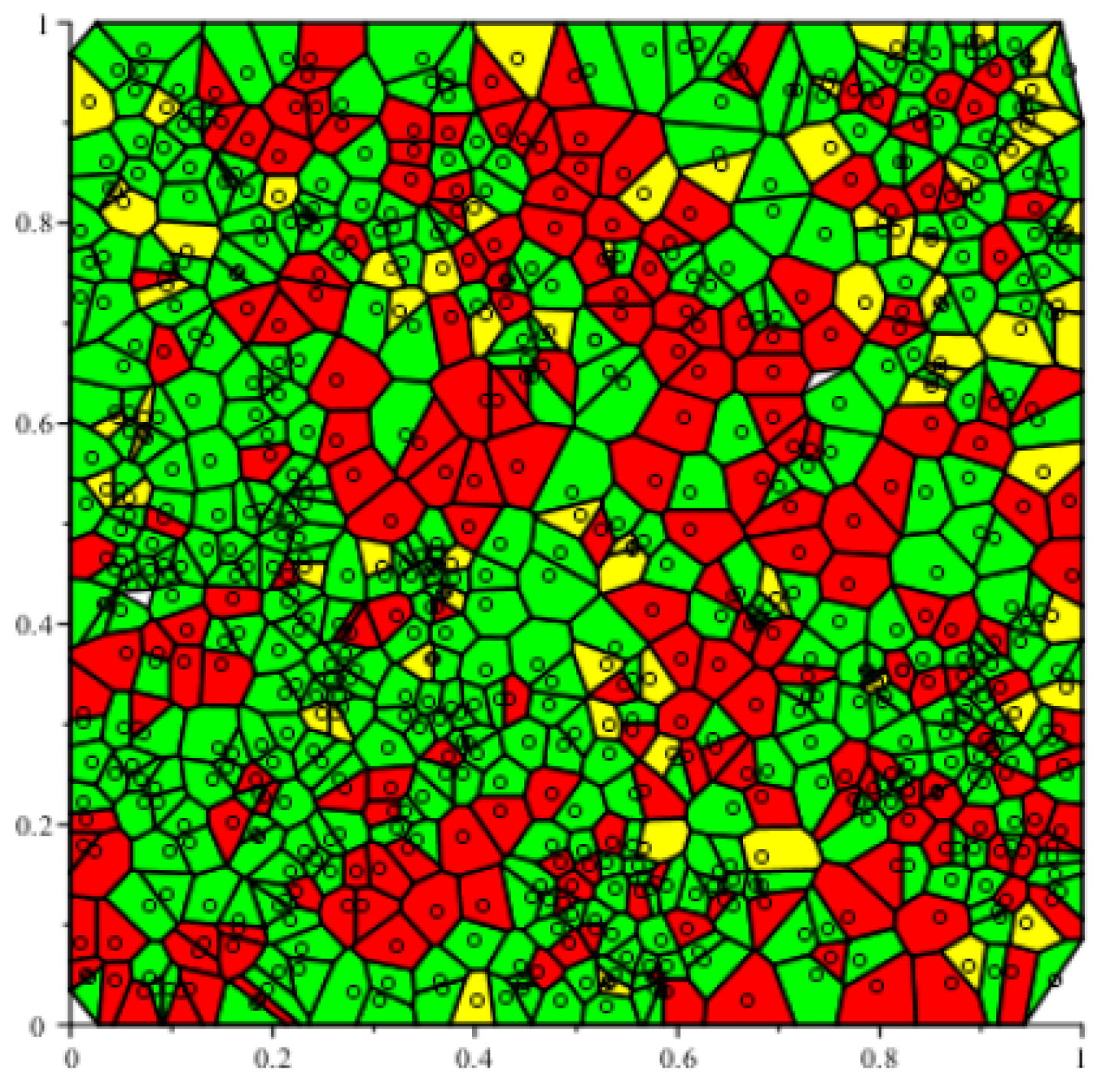
2.2. Study Area and Data

Pine (Pinus sylvestris), spruce (Picea abies), and silver birch (Betula pendula Roth and Betula pubescens Ehrh.) tree stands dominate Lithuanian forests (Lithuanian Statistical Yearbook of Forestry, 2009) and grow at the Arenosol and Podzol forest sites. All the data were collected between 1983 and 2020 across the municipality of Kazlų Rūda in Lithuania. The mean temperatures vary from −16.4 °C in winter to +22° in summer. Precipitation is distributed throughout the year, although it is predominantly in the summer, averaging approximately 680 mm a year. From 1983 to 1987, 53 permanent experimental plots were installed in the forests of the Kazlų Rūda region [11]. Each sample plot consisted of about 0.16–0.72 ha and was remeasured several times, from 1 to 6, at 2- to 37-year intervals. In terms of the regeneration regime, all the plots vary between being naturally regenerated and artificially regenerated and are located in pure or mixed stands. The distribution of the permanent experimental plots can be characterized as follows: pine forests (Pinus sylvestris), 63.8%; spruce (Picea abies), 30.2%; silver birch (Betula pendula Roth and Betula pubescens Ehrh.), 5.8%; and others, 0.2 percent. The age of the ith tree (ranging from all trees to the 10th) in the first measurement cycle was recorded by counting its growth rings in the growth core (for even-aged stands, from the documented records), and the ages of the remaining trees were obtained using the arithmetic mean. The position accuracy of the plane coordinates was 1 dcm, and the diameter measurements were performed by rounding to the nearest 1 mm. The height of approximately every 5th tree was measured, and the height measurements were performed with an accuracy of approximately 1 dcm. Given the two-level measurements, two different datasets were used to obtain the parameter estimates: the first (48 plots; 39,437 mixed-species trees) was used to estimate the fixed-effect parameters for the tree diameter and the potentially available area; see Equations (1) and (2). The second (48 plots; 8604 mixed-species trees) was used to estimate the fixed-effect parameters for the tree height (Equation (3)) to calibrate the random effects (Equation (A2)) and to estimate the correlation matrix of the three-dimensional normal copula by maximizing the pseudo maximum likelihood function defined by Equation (A22). The validation set consisted of 15 plots with 5- and 15-year remeasurement cycles (a total of 2329 tree measurements), in which age, diameter, potentially available area, and height were determined for each measured tree. First of all, a set of validation data was created using only plots with three remeasurement cycles where the time difference between the first and second remeasurement cycles is 5 years and that between the first and third remeasurement cycles is 15 years. If more remeasurement cycles were performed in these validation plots, then the remaining remeasurement cycles of the plot were directed to the evaluation set. The summary of the measurements is presented in

Table 1. Tree age, diameter, potentially available area, and height summary statistics for model estimation and validation datasets *.

Species	Data	Number of Trees	Min	Max	Mean	St. Dev.	Number of Trees	Min	Max	Mean	St. Dev.
Estimation							Validation
Pine	t (year)	24,176	12.0	211.0	56.49	26.75	1531	25.0	119.0	51.88	20.73
	d (cm)	24,176	0.1	61.0	19.30	10.32	1531	5.50	52.80	19.60	7.53
	p (m2)	24,176	0.09	124.19	10.50	8.98	1531	1.20	46.81	9.98	6.48
	h (m)	5346	0.20	37.90	17.29	9.12	1531	6.20	37.50	19.38	5.39
Spruce	t (year)	13,360	12.0	207.0	64.42	25.27	664	7.0	101.0	49.89	16.90
	d (cm)	13,360	0.20	72.20	12.93	8.70	664	3.60	44.80	10.93	5.58
	p (m2)	13,360	0.11	160.24	10.16	8.94	664	0.61	31.15	7.37	5.24
	h (m)	2843	0.50	38.0	12.56	8.52	664	1.0	31.00	11.84	5.34
Birch	t (year)	1761	12.0	127.82	57,49	23.22	133	25.0	75.0	43.24	10.32
	d (cm)	1761	0.90	50.0	15.17	9.42	133	5.10	35.10	16.12	6.59
	p (m2)	1761	0.33	173.82	10.37	8.87	133	1.51	32.55	7.59	4.87
	h (m)	388	0.50	31.90	14.85	8.43	133	7.80	31.0	18.69	5.19
All	t (year)	39,437	12.0	211.0	59.25	26.36	2329	7.0	119.0	50.81	19.35
	d (cm)	39,437	0.1	72.20	16.95	10.22	2329	3.6	52.8	16.93	7.98
	p (m2)	39,437	0.09	173.82	10.37	8.95	2329	0.61	46.81	9.10	6.19
	h (m)	8604	0.20	38.00	15.62	9.16	2329	1.0	37.50	17.19	6.34

* t—age, d—diameter, p—potentially available area (the area of the polygon formed by the Voronoi diagram [3]), h—tree height.

.

3. Results and Discussion

3.1. Parameter Estimates

The fixed-effect parameters of the joint copula-type three-dimensional growth model defined by the cumulative distribution function (A4) are estimated using the pseudo maximum likelihood procedure. In the first step, the fixed-effect parameter vector Ɵ was estimated separately for diameter, the potentially available area, and the height by maximizing an approximated maximum log-likelihood function and using discrete measurements of the tree diameter (x₁), the potentially available area (x₂), and the height (x₃) $\left\{\left(x_{11}^i,x_{21}^i,x_{31}^i\right),\left(x_{12}^i,x_{22}^i,x_{32}^i\right),\dots ,\left(x_{1n_i}^i,x_{2n_i}^i,x_{3n_i}^i\right)\right\}$ at discrete times (ages) $\left\{t_1^i,t_2^i,\dots ,t_{n_i}^i\right\}$ [9]. The measurements of all the observed trees were used to estimate the parameters of the stochastic differential Equations (1) and (2), which determine the growth of the tree diameter and potentially available area, while the parameters of the tree height (Equation (3)) were estimated using a smaller part of the trees that had height measurements (see Table 1). The correlation matrix P of the three-dimensional normal copula-type probability density function defined by (A12) was estimated by maximizing the pseudo maximum likelihood function (A22). The parameter estimates of the stochastic differential Equations (1)–(3) and their standard errors and the parameters of the dependencies for the copula-type probability density function are presented in

Table 2. Parameter estimates for mixed-effect mode of the stochastic differential Equations (1)–(3).

Species	A	Β	ɣ	σ	δ	τj
Diameter
Pine	0.0878	0.0169	−23.5098	0.0006	-	0.0162
Spruce	0.0926	0.0291	−1.5524	0.0102	-	0.0146
Birch	0.2725	0.1060	−0.2137	0.0337	-	0.0679
All	0.0850	0.0226	−7.1108	0.0042	-	0.0069
Potentially available area
Pine	0.0538	0.0157	−1.8435	0.0071	1.5478	0.0076
Spruce	0.0696	0.0230	−0.7630	0.0160	1.7467	0.0125
Birch	0.0669	0.0207	−2.3395	0.0088	1.6375	0.0099
All	0.0617	0.0186	−1.3260	0.0102	1.6151	0.0094
Height
Pine	0.0903	0.0213	−36.7486	0.0001	-	0.0021
Spruce	0.0914	0.0264	−2.1743	0.0062	-	0.0085
Birch	0.2025	0.0577	−12.0370	0.0032	-	0.0147
All	0.0827	0.0213	−13.3459	0.0013	-	0.0043

and

Table 3. Parameter estimates for copula probability density function (19).

Species	𝝆12	𝝆13	𝝆23
Pine	0.1476	0.6964	0.0446
Spruce	0.2083	0.8786	0.1512
Birch	0.1612	0.7854	0.1261
All	0.1513	0.8528	0.0877

, respectively. All the parameter estimates are significant (p < 0.05).

3.2. Analysis of Tree Growth

The foundational aspects of the stochastic differential equation framework of tree growth in a given forest stand can be viewed through the diffusion processes, establishing the one-dimensional probability density functions of the corresponding tree size component and their dependency structure. The functions defined in Equation (7) represent the mean cumulative growth in diameter, the potentially available area, and the height achieved by a tree of a given species at any age in the particular forest stand with growth affecting factors such as artificial thinning, site conditions, changes in temperature, precipitation, or atmospheric CO₂, which are included in the form of random effects. Environmental change has a decisive effect on the growth of the diameter, height, and density (potentially available area), and all these variables also affect each other in the complex form of feedback.

The functions defined in Equations (13) and (14) represent the mean cumulative growth in diameter, the potentially available area, and the height reached by trees of a given species, depending on the values of age and other tree size components in a given forest stand. In this study, we examined in detail the interaction of the components of tree size using the fixed-effect parameter mode (random effects set to zero) (shown in Figure 2), representing three tree species: pine, spruce, and birch. As shown in Figure 2(p1,p2,s1,s2,b1,b2), tree diameter growth is marginally affected by tree potentially available area, but in contrast, diameter growth is significantly affected by height changes. Changes in the height of all tree species are strongly affected by changes in diameter (see Figure 2(p5,s5,b5)), but the potentially available area has a small influence on changes in height (see Figure 2(p6,s6,b6)).

The forestry literature has established that the growth curves of fast-growing forests do not have an inflection point (apparently due to sustained growth) and express a convex shape [26]. Equation (7) has a sigmoidal or convex form and asymptotes. Unfortunately, the growth equation (Equation (7)) does not necessarily have an inflection point, and due to accelerated growth, the inflection point disappears and the growth process takes the form of a convex curve. Forest statisticians have frequently used sigmoidal functions such as logistic, Gompertz, Richards, etc. [27,28]. Graphically, the inflection point can be represented by plotting the second derivative of the diameter, potentially available area, and height growth (Equation (7) (growth acceleration)). The point at which the acceleration curve crosses the abscissa axis indicates the inflection point. Figure 3 illustrates that the growth acceleration curves of the tree diameter, potentially occupied area, and height cross the x-axis when both the fixed- and the mixed-effect modes are used, and the random effects are calibrated using Equation (A2) for all the plots in the validation dataset (among them, 15 plots have pine species trees, 9 have spruce species trees, and 13 have birch species trees).

The forms of the acceleration versus the time equations for both the fixed- and the mixed-effect modes in Figure 3 are in perfect agreement. From the Figure 3(pf1,pm3), it can be seen that the acceleration in the growth of the diameter and height of the pine trees is negative everywhere, meaning that the growth curve is convex and that an inflection point does not exist. The remaining two Figure 3(pm1,pf1), represent the growth acceleration curves of diameter (mixed effect) and height (fixed effect), respectively, of the pine species, showing that the inflection point occurs at a young age and not necessarily in all plots. It would be reasonable to assert that the soils and other environmental conditions in the Kazlų Rūda district are the most suitable for the growth of pine trees. Figure 3(sf1,sf3,sm1,sm3), for spruce trees, show that the diameter and height growth curves have a single inflection point. Additionally, the diameter and height growth acceleration curves for the spruce trees show that there exist two points at which the third derivative of the growth curves is equal to zero; these are referred to as the maximum acceleration point and maximum deceleration point. The maximum acceleration point occurs at a very young age. The diameter growth acceleration curves for the birch trees in Figure 3(pf1,pm1) show that there is a single inflection point, and maximum acceleration and deceleration points. For the birch trees, the height growth acceleration curves presented in Figure 3(pf3,pm3) show that there is no tipping point, and the height growth curve is influenced only by the point of maximum deceleration. The growth acceleration curves of the potentially available area for all the species of trees shown in Figure 3(pf2,sf2,bf2,pm2,sm2,bm2) show that there is an inflection point, and the height growth curve is influenced by the points of maximum acceleration and deceleration.

The relationships between the current and mean annual increments of the tree diameter and the height against the age of the forest stand are illustrated in Figure 4. As seen in Figure 4, the age of a stand exerts a strong influence on the current and mean annual diameter and height increments. From Figure 4, it can be seen that the peaks of the mean annual diameter and height increments are reached even later than those of the current annual increments. The highest current annual increment in tree diameter is reached at about 20–30 years for pine trees (see Figure 4(pf1,pm1)), 30–40 years for spruce trees (see Figure 4(sf1,sm1)), and 10–20 years for birch trees (see Figure 4(bf1,bm1)). The highest current annual increment in tree height occurs until the age of 10 years for pine trees (see Figure 4(pf2,pm2)) 30–40 years for spruce trees (see Figure 4(sf2,sm2)), and until the age of 10 years for birch trees (see Figure 4(bf2,bm2)), respectively. The current annual diameter increment becomes equal to the mean annual increment at 30–50 years of age for pine trees (see Figure 4(pf1,pm1)), 50–70 years of age for spruce trees (see Figure 4(sf1,sm1)), and 20–30 years of age for birch trees (see Figure 4(bf1,bm1)). The increments in diameter and height for birch trees show the highest values for the current annual increment at 1.2 cm (see Figure 4(bf1,bm1)) and 89 cm (see Figure 4(bf2,bm2)), respectively, and at the peak ages of 20 years and 10 years, respectively.

The age at which mean annual increment reaches its peak can be obtained by modifying the relative increment (Equation (19)) by multiplying it by time, t; then, the peak point can be visualized by the point at which this modified curve crosses the line y = 1. Figure 5 visualizes the curve of the relative increment defined by Equation (19) multiplied by time, t, together with the signal line y = 1 for the mixed-effect mode. As can be seen from Figure 5, trees of the pine and birch species reach their peaks of mean annual increment in diameter and height at almost the same age in all the plots in the validation set (see Figure 4(bm2) and Figure 5(pm1,bm1,pm2)). Thus, for the pine trees, the peak of mean annual increment in diameter is reached at approximately 50 years (see Figure 4(pm1)), and in height at approximately 40 years (see Figure 4(pm2)), while for the birch trees, the peak of the mean annual increment in diameter is reached at approximately 27 years (see Figure 4(bm1)), and in height at approximately 30 years (see Figure 4(bm2)). For the spruce trees, the peak of mean annual increment in diameter and height in the investigated plots had values in the intervals of 60–70 and 50–65 (see Figure 4(sm1,sm2)), respectively. The differences in the peaks of the mean annual increment between the plots can be explained by the fact that the conditions of the growing region are unfavorable for the growth of spruce trees, as demonstrated previously in Figure 2 and Figure 4. It should be noted that trees of all species reach their peak mean annual increment in height earlier than in diameter.

It makes sense to link the current annual increment in the tree diameter or height growth (see Equation (15)) to the growth of the diameter or height (see Equations (7), (13) and (14)). Figure 6 shows the linkage of the tree diameter or height with the current increment in the diameter and height growth. Figure 6(p1,s1,b1) show that the current increment in the pine tree diameter reaches its growth peak when the tree diameter reaches 10 cm, and the diameters of the spruce and birch trees reach their current increment peaks when the tree diameter is in the range of 5–15 cm. Likewise, from Figure 6(p2,s2,b2), it can be observed that the current height increments of the pine and spruce trees reach their peak when the tree height reaches 5 m, and the height of the birch tree reaches its current height increment peak when the height of the tree is in the range of 5–15 m.

In this study, using the stochastic differential Equations (1)–(3) and the three-dimensional copula-type distribution function, the three curves for diameter, the potentially available area, and the height were newly derived; for the first curve, the independent variable was only time (see Equation (7)); for the second curve, the independent variables were time and another tree size variable (see Equation (13)); finally, for the third curve, the independent variables were time and the other two remaining tree size variables (see Equation (14)). The goodness of fit of the three presented curves discussed above for modeling the tree diameter, potentially available area, and height is evaluated using statistical measures, and the results are presented in

Table 4. Results of statistical measures * and p-values of Student’s t-test for the individual-tree predictions using the mixed-effect mode.

Curve (Variables)	B (%)	AB (%)	RMSE (%)	R2	T p-Value	Curve (Variables)	B (%)	AB (%)	RMSE (%)	R2	T p-Value
Pine Tree Diameter						Pine Tree Height
Equation (7) (t)	−0.0523 (−6.76)	3.7676 (21.31)	4.8276 (24.63)	0.5891	0.6716	Equation (7) (t)	0.0094 (−2.28)	2.0417 (11.65)	2.7259 (14.06)	0.7441	0.8921
Equation (13) (t, p)	−0.0525 (−6.72)	3.7081 (20.99)	4.8127 (24.56)	0.5916	0.6693	Equation (13) (t, d)	0.0201 (−1.07)	1.3732 (7.59)	1.8684 (9.64)	0.8798	0.6733
Equation (13) (t, h)	−0.0586 (−3.08)	2.4951 (13.16)	3.3515 (17.10)	0.8019	0.4941	Equation (13) (t, p)	0.0081 (−2.30)	2.0428 (11.67)	2.7290 (14.08)	0.7435	0.9040
Equation (13) (t, p, h)	−0.0598 (−3.07)	2.4439 (12.84)	3.3119 (16.90)	0.8066	0.4866	Equation (13) (t, d, p)	0.0214 (−1.03)	1.3647 (7.52)	1.8553 (9.57)	0.8815	0.6508
Pine Tree Potentially Available Area						Spruce Tree Diameter
Equation (7) (t)	−0.1330 (−27.75)	3.6345 (49.64)	4.8685 (48.79)	0.4358	0.2852	Equation (7) (t)	−0.7109 (−14.84)	3.1111 (32.20)	4.3715 (39.97)	0.3702	0.0001
Equation (13) (t, d)	−0.1270 (−27.22)	3.6019 (49.05)	4.8270 (48.37)	0.4454	0.3034	Equation (13) (t, p)	−0.5898 (−13.70)	2.8473 (29.85)	4.0189 (36.75)	0.4702	0.0002
Equation (13) (t, h)	−0.0864 (−36.59)	3.8832 (60.09)	5.9846 (63.67)	0.4445	0.1800	Equation (13) (t, h)	−0.2101 (−3.12)	1.4505 (14.29)	2.1234 (19.42)	0.8538	0.0110
Equation (13) (t, d, h)	−0.0775 (−35.72)	3.8191 (59.12)	5.9044 (62.82)	0.4593	0.2229	Equation (13) (t, p, h)	−0.2032 (−3.05)	1.3917 (13.77)	2.0059 (18.34)	0.8695	0.0092
Spruce Tree Height						Spruce Tree Potentially Available Area
Equation (7) (t)	−0.4554 (−13.65)	3.0009 (31.30)	4.0033 (33.82)	0.4309	0.0035	Equation (7) (t)	−0.0902 (−50.87)	3.6998 (5.0414)	5.0114 (68.39)	0.0737	0.6448
Equation (13) (t, d)	0.0029 (−4.52)	1.4286 (15.20)	1.8768 (15.85)	0.8765	0.9682	Equation (13) (t, d)	−0.0370 (−47.16)	3.5327 (73.93)	4.7696 (64.70)	0.1711	0.8416
Equation (13) (t, p)	−0.3581 (−13.11)	2.8746 (30.40)	3.8185 (32.26)	0.4844	0.0160	Equation (13) (t, h)	−0.0558 (−49.12)	3.6247 (76.41)	4.9000 (66.47)	0.1251	0.7691
Equation (13) (t, d, p)	0.0024 (−4.49)	1.4145 (15.07)	1.8656 (15.76)	0.8780	0.9732	Equation (13) (t, d, h)	−0.0366 (−46.64)	3.5100 (73.27)	4.7422 (64.33)	0.1806	0.8425
Birch Tree Diameter						Birch Tree Height
Equation (7) (t)	−0.1782 (−13.61)	3.91.9 (31.24)	4.8552 (30.11)	0.4568	0.6739	Equation (7) (t)	−0.0788 (−5.45)	2.7530 (17.44)	3.5389 (18.93)	0.5293	0.7984
Equation (13) (t, p)	−0.1535 (−13.27)	3.8440 (30.73)	4.8083 (29.79)	0.4683	0.7140	Equation (13) (t, d)	−0.1668 (−1.93)	1.3747 (7.92)	1.7571 (9.40)	0.8830	0.2772
Equation (13) (t, h)	0.0969 (−3.92)	2.1346 (14.93)	2.7308 (16.93)	0.8282	0.6839	Equation (13) (t, p)	−0.0735 (−5.42)	2.7269 (17.33)	3.5634 (19.06)	0.5228	0.8129
Equation (13) (t, p, h)	0.1013 (−3.87)	2.1098 (14.76)	2.7082 (16.79)	0.8310	0.6679	Equation (13) (t, d, p)	−0.1668 (−1.93)	1.3745 (7.92)	1.7569 (9.40)	0.8830	0.2771

* Statistical measures: the mean bias, B (the percentage mean bias, $\%B$); the absolute mean bias, AB (the percentage absolute mean bias, $\%AB$); the root mean square error, RMSE (the percentage root mean square error, $\%RMSE$); and the coefficient of determination, R², defined by Equations (21)–(24).

using a validation dataset. The statistical measures presented in Table 4 show that the proposed models best corresponded to the observed validation dataset of the pine trees in uneven-aged mixed-species stands. The predictions of the pine tree heights showed stable and high statistical measures; for example, the mean bias did not exceed 0.02 m (−1.03%); the absolute mean bias did not exceed 1.36 m (7.52%); the root mean square error did not exceed 1.85 m (9.57%); and the coefficient of determination reached to as high as 88.2%. The pine tree diameter predictions showed slightly lower statistical measures, and the tree potentially occupied area predictions showed a lower performance on the statistical measures compared to the tree height predictions. It should be noted that the predictions of the diameter, height, and potentially available area for spruce trees generated the lowest statistical measures among the tree species. Additionally, it can be stated that the statistical measures of the predictions of the potentially available area were the lowest compared to the predictions of the height and diameter, and the additional variable diameter or height increased the statistical measures slightly. Furthermore, with the introduction of an additional independent variable, the tree potentially available area, into the tree height or diameter curve, the increase in the statistical measures is negligible, and in contrast, the inclusion of the tree diameter and height in the relationship of the potentially available area does not show a significant effect.

$$B=\frac{1}{n}{{\displaystyle \sum }}_{i=1}^n\left(y_i-\stackrel{\wedge }{y_i}\right), (\%B=\frac{1}{n}{{\displaystyle \sum }}_{i=1}^n\frac{y_i-\stackrel{\wedge }{y_i}}{y_i}\ast 100),$$

(21)

$$AB=\frac{1}{n}{{\displaystyle \sum }}_{i=1}^n\left|y_i-\stackrel{\wedge }{y_i}\right|, (\%B=\frac{1}{n}{{\displaystyle \sum }}_{i=1}^n\left|\frac{y_i-\stackrel{\wedge }{y_i}}{y_i}\right|\ast 100),$$

(22)

$$RMSE=\sqrt{\frac{1}{n}{{\displaystyle \sum }}_{i=1}^n{\left(y_i-\stackrel{\wedge }{y_i}\right)}^2}, (\%RMSE=\sqrt{\frac{1}{n}{{\displaystyle \sum }}_{i=1}^n{(\frac{y_i-\stackrel{\wedge }{y_i}}{y_i})}^2}\ast 100),$$

(23)

$$R^2=1-\frac{{{\displaystyle \sum }}_{i=1}^n{\left(y_i-\stackrel{\wedge }{y_i}\right)}^2}{{{\displaystyle \sum }}_{i=1}^n{(y_i-\overline{y})}^2}.$$

(24)

Table 5. Results of statistical measures and p-values of Student’s t-test for whole-stand predictions using the mixed-effect model.

Curve (Variables)	B (%)	AB (%)	RMSE (%)	R2	T p-Value	Curve (Variables)	B (%)	AB (%)	RMSE (%)	R2	T p-Value
Pine Tree Diameter						Pine Tree Height
Equation (7) (t)	0.0137 (0.02)	0.9450 (4.23)	1.4187 (6.38)	0.9318	0.9489	Equation (7) (t)	−0.1262 (−0.52)	0.5926 (2.76)	0.8655 (4.08)	0.9620	0.3385
Equation (13) (t, p)	−0.1319 (−0.63)	0.9479 (4.18)	1.3652 (6.14)	0.9363	0.5247	Equation (13) (t, d)	−0.2203 (−1.02)	0.3980 (1.85)	0.5834 (2.75)	0.9807	0.0160
Equation (13) (t, h)	0.2499 (1.00)	0.5783 (2.61)	0.8827 (3.97)	0.9715	0.0669	Equation (13) (t, p)	−0.1513 (−0.64)	0.5889 (2.73)	0.8621 (4.07)	0.9620	0.2505
Equation (13) (t, p, h)	0.1306 (0.46)	0.5367 (2.47)	0.8347 (3.75)	0. 9758	0.3051	Equation (13) (t, d, p)	−0.1879 (−0.86)	0.3918 (1.83)	0.5776 (2.72)	0.9817	0.0364
Pine Tree Potentially Available Area						Spruce Tree Diameter
Equation (7) (t)	−0.1371 (−1.43)	0.8767 (8.01)	1.2111 (11.03)	0.9265	0.4567	Equation (7) (t)	−0.7202 (−5.74)	1.1156 (9.56)	1.1587 (9.20)	0.8837	0.0047
Equation (13) (t, d)	−0.1622 (−1.62)	0.8050 (7.43)	1.1211 (10.21)	0.9365	0.3423	Equation (13) (t, p)	−0.9502 (−7.81)	1.3568 (11.19)	1.2785 (10.15)	0.8415	0.0010
Equation (13) (t, h)	−0.1294 (−1.36)	0.8629 (7.91)	1.1905 (10.85)	0.9290	0.4745	Equation (13) (t, h)	−0.0306 (−0.14)	0.8023 (6.40)	1.0270 (8.15)	0.9340	0.8713
Equation (13) (t, d, h)	−0.1906 (−35.72)	0.7973 (7.32)	1.1201 (10.20)	0.9361	0.2650	Equation (13) (t, p, h)	−0.1389 (−1.02)	0.8442(6.61)	1.0505 (8.34)	0.9299	0.5145
Spruce Tree Height						Spruce Tree Potentially Available Area
Equation (7) (t)	−0.6456 (−5.18)	1.0927 (8.50)	1.4656 (11.56)	0.7857	0.0371	Equation (7) (t)	0.1726 (−1.81)	1.3916 (13.67)	1.9892 (19.75)	0.8789	0.6689
Equation (13) (t, d)	−0.3298 (−3.01)	0.7273 (5.79)	0.9914 (7.82)	0.9089	0.1086	Equation (13) (t, d)	0.1667 (−2.07)	1.3726 (13.52)	1.9766 (19.63)	0.8803	0.6767
Equation (13) (t, p)	−0.8052 (−9.57)	1.1729 (9.19)	1.5147 (11.94)	0.7541	0.0135	Equation (13) (t, h)	0.1931 (−1.77)	1.4267 (14.02)	2.0112 (19.98)	0.8758	0.6353
Equation (13) (t, d, p)	−0.2877 (−2.66)	0.7246 (5.73)	0.9878 (7.79)	0.9116	0.1577	Equation (13) (t, d, h)	0.1511 (−2.24)	1.3364 (13.15)	1.9744 (19.61)	0.8807	0.7051
Birch Tree Diameter						Birch Tree Height
Equation (7) (t)	0.3437 (1.72)	1.1631 (6.86)	1.4458 (8.03)	0.8958	0.2556	Equation (7) (t)	0.1826 (0.61)	0.8385 (4.53)	0.9437 (4.90)	0.9412	0.3526
Equation (13) (t, p)	0.0591 (0.03)	1.2562 (7.27)	1.4959 (8.31)	0.8943	0.8481	Equation (13) (t, d)	−0.5721 (−3.38)	0.7000 (3.94)	0.6981 (3.63)	0.9476	0.0004
Equation (13) (t, h)	0.5554 (3.24)	0.9046 (5.14)	1.0379 (5.77)	0.9344	0.0151	Equation (13) (t, p)	0.0041 (−0.42)	0.8570 (4.67)	0.9856 (5.12)	0.9382	0.9836
Equation (13) (t, p, h)	0.4326 (2.54)	0.8625 (4.87)	1.0415 (5.78)	0.9400	0.0530	Equation (13) (t, d, p)	−0.5783 (−3.37)	0.6992 (3.94)	0.6980 (3.63)	0.9477	0.0001

summarizes the statistical measures of the stand mean diameter, potentially available area, and height curves (7), (13), and (14). All of the mean diameter, potentially available area, and height models of a stand used, as defined by Equations (7), (13), and (14), produced predictions that showed a significantly higher level of statistical measures compared to the accuracy of individual-tree predictions assessed by the same statistical measures and presented in Table 4. The best statistical measures were demonstrated by model (14), defining the mean height of the pine trees in the stand as a function of the average age of the stand, the average diameter of the pine trees in the stand, and the average potentially available area of the pine trees in the stand. The predictions for the mean height of the pine trees in the stand demonstrated that the statistical measure for mean bias did not exceed −0.17 m (−0.86%), absolute mean bias did not exceed 0.39 m (1.83%), root mean square error did not exceed 0.58 m (2.72%), and the coefficient of determination reached as high as 98.2%.

3.3. Evolution of the Number of Trees

Environmental resources can only satisfy a limited number of trees in a stand; therefore, the number of trees gradually decreases with increasing tree diameter and height, depending on the intensity of interspecific competition. To model the number of trees per hectare during the development of a stand, the link between the number of trees per hectare and the mean potentially available area, diameter, and height was determined using the mean trend Equations (7), (13), and (14), as follows:

$$N^i\left(t|t_{in},x_{2 in},\widehat{\mathsf{\theta }}, \widehat{{\varphi }_p^i}\right)={{\displaystyle \int }}_{{\mathrm{ɣ}}_p}^{+\infty }{k}_s^i\frac{10,000.}{x_p}{f}_p^i\left(x_p,t|t_{in},x_{2 in},\widehat{\mathsf{\theta }}, \widehat{{\varphi }_p^i}\right)d{x}_p, i=1, 2, \dots , K,$$

(25)

$$\begin{gathered} N^i\left(t, x_d|t_{in},x_{d in},x_{p in},\widehat{\mathsf{\theta }}, \widehat{{\varphi }_d^i}, \widehat{{\varphi }_p^i},\widehat{{\rho }_{dp}}\right) \\ ={{\displaystyle \int }}_{{\mathrm{ɣ}}_p}^{+\infty }{k}_s^i{\frac{10,000.}{x_p}}_p^i{f}_{p|d}^i\left(x_p,t|x_d,t_{in},x_{d in},x_{p in},\widehat{\mathsf{\theta }}, \widehat{{\varphi }_d^i}, \widehat{{\varphi }_p^i},\widehat{{\rho }_{dp}}\right)d{x}_p, i=1, 2, \dots , K, \end{gathered}$$

(26)

$$\begin{gathered} N^i\left(t, x_h|t_{in},x_{p in},x_{h in},\widehat{\mathsf{\theta }}, \widehat{{\varphi }_p^i}, \widehat{{\varphi }_h^i},\widehat{{\rho }_{ph}}\right) \\ ={{\displaystyle \int }}_{{\mathrm{ɣ}}_p}^{+\infty }{k}_s^i{\frac{10,000.}{x_p}}_p^i{f}_{p|d}^i\left(x_p,t|x_h,t_{in},x_{p in},x_{h in},\widehat{\mathsf{\theta }}, \widehat{{\varphi }_p^i}, \widehat{{\varphi }_h^i},\widehat{{\rho }_{ph}}\right)d{x}_p, i=1, 2, \dots , K, \end{gathered}$$

(27)

$$\begin{gathered} N^i\left(t,x_d, x_h|t_{in},x_{d in},x_{p in},x_{h in}\widehat{\mathsf{\theta }}, \widehat{{\varphi }_d^i}, \widehat{{\varphi }_p^i},\widehat{{\varphi }_h^i},\widehat{P}\right) \\ ={{\displaystyle \int }}_{{\mathrm{ɣ}}_p}^{+\infty }{k}_s^i{\frac{10,000.}{x_p}}_p^i{f}_{p|dh}^i\left(x_p,t|x_d,x_h,t_{in},x_{d in},x_{p in},x_{h in},\widehat{\mathsf{\theta }},\widehat{{\varphi }_d^i}, \widehat{{\varphi }_p^i}, \widehat{{\varphi }_h^i},\widehat{P}\right)d{x}_p, \\ i=1,2,\dots ,K, \end{gathered}$$

(28)

where K is the number of observed plots in the validation dataset; $k_s^l$is the part of the stand occupied by the tree species concerned ($k_{all}^l=1$, $0\le k_{pine}^l\le 1$, 0 $\le k_{spruce}^l\le 1$, 0 $\le k_{birch}^l\le 1$); the estimates of the fixed-effect parameters $\widehat{\mathsf{\theta }}$ are taken from Table 2; the estimates of the dependency parameters $\widehat{ P}$, $\widehat{{\rho }_{dp}}$, and $\widehat{{\rho }_{ph}}$ are taken from Table 3; the random effects $\widehat{{\varphi }_d^i}, \widehat{{\varphi }_p^i}, \widehat{{\varphi }_h^i}$ are calibrated by Equation (A2) using the validation dataset; for the prediction mode, $t_{in}=4,x_{d in}=0.1,x_{p in}=\widehat{ \delta } ,x_{h in}=0.4$ (where $\widehat{ \delta }$ was taken from Table 2); and for the forecast mode, $t_{in}$, $x_{d in},x_{p in} ,x_{h in}$ are the average values of the first cycle measurements of age, diameter, potentially available area, and height. The evolution of the number of trees per hectare of a particular stand against age for all species and pine, spruce, and birch trees and four different stands is shown in Figure 7. The results of the statistical measures of the number of trees per hectare predictions are presented in

Table 6. Results of statistical measures and p-values of Student’s t-test for predictions of the number of trees per hectare using the mixed-effect mode.

Curve (Variables)	B (%)	AB (%)	RMSE (%)	R2	T p-Value	Curve (Variables)	B (%)	AB (%)	RMSE (%)	R2	T p-Value
Number of All Trees per ha						Number of Pine Trees per ha
Equation (25) (t)	25.21 (2.48)	83.19 (7.78)	103.01 (9.09)	0.9423	0.1116	Equation (25) (t)	25.40 (4.97)	65.95 (9.80)	84.40 (11.80)	0.9468	0.0521
Equation (26) (t, d)	37.91 (3.42)	80.13 (7.48)	94.71 (8.36)	0.9466	0.0110	Equation (26) (t, d)	30.50 (5.50)	66.09 (9.81)	80.97 (11.32)	0.9487	0.0163
Equation (27) (t, h)	29.56 (2.75)	81.77 (7.65)	99.30 (8.76)	0.9450	0.0545	Equation (27) (t, h)	26.66 (5.07)	66.04 (9.82)	83.15 (11.62)	0.9477	0.0391
Equation (28) (t, d, h)	44.49 (3.99)	81.81 (7.59)	94.53 (8.34)	0. 9440	0.0032	Equation (28) (t, d, h)	32.89 (5.88)	67.03 (9.94)	81.76 (11.43)	0.9468	0.0106
Number of Spruce Trees per ha						Number of Birch Trees per ha
Equation (25) (t)	−25.09 (−7.19)	69.48 (14.45)	108.44 (19.03)	0.9367	0.2581	Equation (25) (t)	1.50 (−5.47)	17.22 (18.27)	22.27 (15.80)	0.9684	0.7437
Equation (26) (t, d)	−22.97 (−6.69)	61.56 (13.31)	94.47 (16.58)	0.9517	0.2353	Equation (26) (t, d)	4.46 (−3.58)	18.06 (17.94)	23.59 (16.74)	0.9634	0.3635
Equation (27) (t, h)	−25.57 (−7.16)	65.93 (13.95)	99.81 (17.52)	0.9458	0.2118	Equation (27) (t, h)	2.17 (−4.89)	17.10 (18.0)	22.25 (15.79)	0.9683	0.6369
Equation (28) (t, d, h)	−21.39 (−6.49)	62.38 (13.35)	95.09 (16.69)	0.9515	0.2714	Equation (28) (t, d, h)	4.47 (−3.57)	18.07 (17.94)	23.60 (16.75)	0.9634	0.3624

. The statistical measures of the number of trees per hectare for the forecast mode are presented in

Table 7. Results of statistical measures and p-values of Student’s t-test for forecasts of the number of trees per hectare using the mixed-effect mode and Equation (25).

Curve (Variables)	B (%)	AB (%)	RMSE (%)	R2	T p-Value	Curve (Variables)	B (%)	AB (%)	RMSE (%)	R2	T p-Value
5-Year Forecast Period						15-Year Forecast Period
Equation (25) (t)	25.21 (2.48)	83.19 (7.78)	103.01 (9.09)	0.9423	0.1116	Equation (25) (t)	25.40 (4.97)	65.95 (9.80)	84.40 (11.80)	0.9468	0.0521
Equation (26) (t, d)	37.91 (3.42)	80.13 (7.48)	94.71 (8.36)	0.9466	0.0110	Equation (26) (t, d)	30.50 (5.50)	66.09 (9.81)	80.97 (11.32)	0.9487	0.0163
Equation (27) (t, h)	29.56 (2.75)	81.77 (7.65)	99.30 (8.76)	0.9450	0.0545	Equation (27) (t, h)	26.66 (5.07)	66.04 (9.82)	83.15 (11.62)	0.9477	0.0391
Equation (28) (t, d, h)	44.49 (3.99)	81.81 (7.59)	94.53 (8.34)	0. 9440	0.0032	Equation (28) (t, d, h)	32.89 (5.88)	67.03 (9.94)	81.76 (11.43)	0.9468	0.0106

. Figure 7 shows that the model curve of the number of trees per hectare defined by Equation (25) corresponds well to the measurement data from the validation dataset. The best fitness of the predictions of the number of trees per hectare was confirmed by all the statistical measures for the trees of the pine species, while the aforementioned statistical measures were the worst for the trees of the spruce species. Table 6 and Table 7 demonstrate the higher goodness-of-fit statistical measures compared to those achieved using the generalized algebraic difference approach, which is the one used traditionally [29]. The statistical measures computed in Table 6 and Table 7 for the number of trees per hectare models, with the additional explanatory variables for diameter and height, indicated a slight improvement in prediction accuracy, with a lower performance of the first model, as expected. Therefore, as demonstrated in Table 6 and Table 7, the maximum impact on the tree density dynamics demonstrated the tree potentially available area and age.

The number of trees per hectare varies with the mean diameter, height, and volume of the stand. Stands of small mean diameter, height, or volume have a large number of trees, while stands of large mean diameter, height, or volume have relatively few [30]. The relationship between the mean diameter, height, and volume (increasing over age) and the number of live trees per hectare (decreasing over age) can been described by means of a “limiting relationship” [31]. The intensity of competition between trees varies with the initial number of trees per hectare, as shown in Figure 7. The process of self-thinning (decay) in the different stands shown in Figure 7 indicates that the stands formed with different initial densities do not thin to the same final number of trees per hectare (see Figure 7a–d). The process of the current rate of the decay of the number of trees per hectare, expressed as the ratio of the current annual decay (Equation (15)) to the number of trees per hectare (Equation (25)), is shown in Figure 8. From Figure 8a–d, we can state that the decay process drops to 1% for the pine species trees at approximately 100 years; for the spruce species trees at 80 years; and finally at 70 years for the birch species trees. It should be noted that the soil characteristics of this region are not favorable for spruce trees.

4. Conclusions

Forest system data are characterized by important features such as dynamism, uncertainty, stochasticity, deviation of variables from the normal distribution, multicollinearity, and false correlations, which complicate the modeling and prediction of forest systems. Generally, forestry researchers treat probabilistic modeling as the mathematical study of an observed random variable, such as tree diameter, height, etc. The theory of stochastic processes enables the description of the evolution of random variables with respect to time, which plays an important role in the study of various growth processes in a forest stand. Stochastic processes, in a sense, could be referred to as the dynamic part of probability theory. Our previous works used the multi-dimensional stochastic process paradigm, where for parameter estimates a lot of computing resources are consumed. Linking one-dimensional stochastic processes according to the copula function reduced the volume of computer calculations and made it possible to analyze the growth processes of various trees, stands and their connections in the form of nonlinear equations.

References

1. Zeide, B. Analysis of Growth Equations. For. Sci. 1993, 39, 594–616. [Google Scholar] [CrossRef]
2. Petrauskas, E.; Rupšys, P.; Narmontas, M.; Aleinikovas, M.; Beniušienė, L.; Šilinskas, B. Stochastic Models to Qualify Stem Tapers. Algorithms 2020, 13, 94. [Google Scholar] [CrossRef] [Green Version]
3. Rupšys, P.; Petrauskas, E. Symmetric and Asymmetric Diffusions through Age-Varying Mixed-Species Stand Parameters. Symmetry 2021, 13, 1457. [Google Scholar] [CrossRef]
4. Suzuki, T. Forest transition as a stochastic process (I). J. Jpn. For. Sci. 1966, 48, 436–439. [Google Scholar]
5. Sloboda, B. Kolmogorow–Suzuki und die stochastische Differentialgleichung als Beschreibungsmittel der Bestandesevolution. Mitt Forstl Bundes Vers. Wien 1977, 120, 71–82. [Google Scholar]
6. Garcia, O. Modelling stand development with stochastic differential equations. In Mensuration for Management Planning of Exotic Forest Plantations; Elliot, D.A., Ed.; New Zealand Forest Service, Forest Research Institute Symposium: Rotorua, New Zealand, 1979; 20, pp. 315–333. [Google Scholar]
7. Tanaka, K. A stochastic model of height growth in an even-aged pure forest stand—why is the coefficient of variation of the height distribution smaller than that of the diameter distribution. J. Jpn. For. Soc. 1988, 70, 20–29. [Google Scholar]
8. Rennolls, K. Forest height growth modelling. For. Ecol. Manag. 1995, 71, 217–225. [Google Scholar] [CrossRef]
9. Rupšys, P. New insights into tree height distribution based on mixed-effects univariate diffusion processes. PLoS ONE 2016, 11, e0168507. [Google Scholar] [CrossRef]
10. Narmontas, M.; Rupšys, P.; Petrauskas, E. Construction of Reducible Stochastic Differential Equation Systems for Tree Height–Diameter Connections. Mathematics 2020, 8, 1363. [Google Scholar] [CrossRef]
11. Rupšys, P.; Petrauskas, E. Analysis of Longitudinal Forest Data on Individual-Tree and Whole-Stand Attributes Using a Stochastic Differential Equation Model. Forests 2022, 13, 425. [Google Scholar] [CrossRef]
12. Rupšys, P. Stochastic Mixed-Effects Parameters Bertalanffy Process, with Applications to Tree Crown Width Modeling. Math. Probl. Eng. 2015, 2015, 375270. [Google Scholar] [CrossRef] [Green Version]
13. Rupšys, P. Understanding the Evolution of Tree Size Diversity within the Multivariate nonsymmetrical Diffusion Process and Information Measures. Mathematics 2019, 7, 761. [Google Scholar] [CrossRef] [Green Version]
14. Petrauskas, E.; Bartkevičius, E.; Rupšys, P.; Memgaudas, R. The use of stochastic differential equations to describe stem taper and volume. Baltic For. 2013, 19, 43–151. [Google Scholar]
15. Narmontas, M.; Rupšys, P.; Petrauskas, E. Models for Tree Taper Form: The Gompertz and Vasicek Diffusion Processes Framework. Symmetry 2020, 12, 80. [Google Scholar] [CrossRef]
16. Rupšys, P. Generalized fixed-effects and mixed-effects parameters height–diameter models with diffusion processes. Int. J. Biomath. 2015, 8, 1550060. [Google Scholar] [CrossRef]
17. Rupšys, P. Modeling Dynamics of Structural Components of Forest Stands Based on Trivariate Stochastic Differential Equation. Forests 2019, 10, 506. [Google Scholar] [CrossRef] [Green Version]
18. Rupšys, P.; Petrauskas, E. On the Construction of Growth Models via Symmetric Copulas and Stochastic Differential Equations. Symmetry 2022, 14, 2127. [Google Scholar] [CrossRef]
19. Wang, M.; Upadhyay, A.; Zhang, L. Trivariate distribution modeling of tree diameter, height, and volume. For. Sci. 2010, 56, 290–300. [Google Scholar]
20. Sklar, M. Fonctions de repartition an dimensions et leurs marges. Publ. Inst. Statist. Univ. Paris 1959, 8, 229–231. [Google Scholar]
21. Rupšys, P.; Petrauskas, E. Evolution of Bivariate Tree Diameter and Height Distribution via Stand Age: Von Bertalanffy Bivariate Diffusion Process Approach. J. For. Res. 2019, 24, 16–26. [Google Scholar] [CrossRef]
22. Rupšys, P.; Narmontas, M.; Petrauskas, E. A Multivariate Hybrid Stochastic Differential Equation Model for Whole-Stand Dynamics. Mathematics 2020, 8, 2230. [Google Scholar] [CrossRef]
23. Rupšys, P.; Petrauskas, E. A Linkage among Tree Diameter, Height, Crown Base Height, and Crown Width 4-variate Distribution and Their Growth Models: A 4-variate Diffusion Process Approach. Forests 2017, 8, 479. [Google Scholar] [CrossRef] [Green Version]
24. Ishihara, M.I.; Konno, Y.; Umeki, K.; Ohno, Y.; Kikuzawa, K. A new model for size-dependent tree growth in forests. PLoS ONE 2016, 11, e0152219. [Google Scholar] [CrossRef] [Green Version]
25. Itô, K. Stochastic integral. Proc. Imp. Acad. 1944, 20, 519–524. [Google Scholar] [CrossRef]
26. Yuancai, L.; Marques, C.; Macedo, F. Comparison of Schnute’s and Bertalanffy-Richards’ growth functions. For. Ecol. Manag. 1997, 96, 283–288. [Google Scholar] [CrossRef]
27. Monti, C.A.U.; Oliveira, R.M.; Roise, J.P.; Scolforo, H.F.; Gomide, L.R. Hybrid Method for Fitting Nonlinear Height–Diameter Functions. Forests 2022, 13, 1783. [Google Scholar] [CrossRef]
28. Rodrigo, M.; Zulkarnaen, D. Mathematical Models for Population Growth with Variable Carrying Capacity: Analytical Solutions. AppliedMath 2022, 2, 466–479. [Google Scholar] [CrossRef]
29. Gómez-García, E.; Crecente-Campo, F.; Tobin, B.; Hawkins, M.; Nieuwenhuis, M.; Diéguez-Aranda, U. A dynamic volume and biomass growth model system for even-aged downy birch stands in south-western Europe. Forestry 2014, 87, 165–176. [Google Scholar] [CrossRef]
30. Clutter, J.L.; Bennett, F.A. Diameter Distributions in Old-Field Slash Pine Plantations; Georgia Forest Research Council: Atlanta, GA, USA, 1965; Volume 13, p. 9. [Google Scholar]
31. Reineke, L.H. Perfecting a stand-density index for evenaged forests. J. Agric. Res. 1933, 46, 627–638. [Google Scholar]
32. Rupšys, P. The use of copulas to practical estimation of multivariate stochastic differential equation mixed effects models. AIP Conf. Proc. 2015, 1684, 080011. [Google Scholar]
33. Rupšys, P. Univariate and Bivariate Diffusion Models: Computational Aspects and Applications to Forestry. In Stochastic Differential Equations: Basics and Applications; Tony, G.D., Ed.; Nova Science Publisher’s: New York, NY, USA, 2018; pp. 1–77. [Google Scholar]
Figure 1. Tree potentially available area for randomly selected plot: 1983rd year cycle of measurement (mean age, 50.38 years); red—Scots pine trees; green—Norway spruce trees; yellow—birch trees; circles—tree position.
Forests 14 00012 g001
Figure 2. Relationships between components of two tree sizes at a particular age: solid black line—20 years; solid blue line—60 years; solid red line—120 years; (p1p6) pine trees; (s1s6) spruce trees; (b1b6) birch trees; (p1,s1,b1) diameter growth against potentially available area; (p2,s2,b2) diameter growth against height; (p3,s3,b3) potentially available area growth against diameter; (p4,s4,b4) potentially available area growth against height; (p5,s5,b5) height growth against diameter; (p6,s6,b6) height growth against potentially available area.
Forests 14 00012 g002
Figure 3. Acceleration of tree diameter, potentially available area, and height growth for both the fixed- and the mixed-effect modes via age: (pf1pf3,sf1sf3,bf1bf3) fixed-effect mode; (pm1pm3,sm1sm3,bm1bm3) mixed-effect mode; (pf1pf3,pm1pm3) pine trees; (sf1sf3,sm1sm3) spruce trees; (bf1bf3,bm1bm3) birch trees; first column—diameter; second column—potentially available area; third column—height.
Forests 14 00012 g003
Figure 4. Current and mean annual increments of tree diameter and height growth for both the fixed- and the mixed-effect modes via age: (pf1,pf2,sf1,sf2,bf1,bf2) fixed-effect mode; (pm1,pm2,sm1,sm2,bm1,bm2) mixed-effect mode; (pf1,pf2,pm1,pm2) pine trees; (sf1,sf2,sm1,sm2) spruce trees; (bf1,bf2,bm1,bm2) birch trees; first column—diameter; second column—height; black—first stand; blue—second stand; red—third stand; solid line—current annual increment; dotted line—mean annual increments.
Forests 14 00012 g004aForests 14 00012 g004b
Figure 5. Relative increments multiplied by time of tree diameter, and height growth along with the signal line y = 1: (pm1,pm2) pine trees; (sm1,sm2) spruce trees; (bm1,bm2) birch trees; first column—diameter; second column—height; black—first stand; blue—second stand; red—third stand; dashed line—signal line; black—first stand; blue—second stand; red—third stand.
Forests 14 00012 g005
Figure 6. Linkage of current increments of tree diameter and height growth with mean diameter and height: (p1,p2) pine trees; (s1,s2) spruce trees; (b1,b2) birch trees; first column—diameter; second column—height; black—first stand; blue—second stand; red—third stand.
Forests 14 00012 g006
Figure 7. Evolution of the number of trees per hectare for three randomly selected stands: black—first stand; blue—second stand; red—third stand; (a) all trees; (b) pine trees ( k p i n e 1 = 0.97 in black, k p i n e 2 = 0.25 in blue; k p i n e 3 = 0.73 in red); (c) spruce trees ( k s p r u c e 1 = 0.05 in black, k s p r u c e 2 = 0.72 in blue; k s p r u c e 3 = 0.31 in red); (d) birch tree ( k b i r c h 1 = 0.22 in black, k b i r c h 2 = 0.16 in blue; k b i r c h 3 = 0.05 in red).
Forests 14 00012 g007
Figure 8. Evolution of the relative annual decay process of the number of trees per hectare for three randomly selected stands: black—first stand; blue—second stand; red—third stand; (a) all trees; (b) pine trees ( k p i n e 1 = 0.97 in black, k p i n e 2 = 0.25 in blue; k p i n e 3 = 0.73 in red); (c) spruce trees ( k s p r u c e 1 = 0.05 in black, k s p r u c e 2 = 0.72 in blue; k s p r u c e 3 = 0.31 in red); (d) birch tree ( k b i r c h 1 = 0.22 in black, k b i r c h 2 = 0.16 in blue; k b i r c h 3 = 0.05 in red).
Forests 14 00012 g008