Article

Heat Budget of Sub-Mediterranean Downy Oak Landscapes of Southeastern Crimea

A.O. Kovalevsky Institute of Biology of the Southern Seas of RAS, 299011 Sevastopol, Russia
*
Author to whom correspondence should be addressed.
Forests 2023, 14(10), 1927; https://doi.org/10.3390/f14101927
Submission received: 22 August 2023 / Revised: 18 September 2023 / Accepted: 19 September 2023 / Published: 22 September 2023
(This article belongs to the Special Issue Forest Microclimate: Predictions, Drivers and Impacts)

Abstract

:
This article presents the findings of a research endeavor focused on the diurnal and seasonal dynamics of heat balance and its constituent elements within an oak forest situated in the expanse of the Karadag Nature Reserve. Computed are the values corresponding to the elements of heat balance, encompassing radiation balance, latent heat fluxes corresponding to heat consumption for evaporation, turbulent heat exchange transpiring within the atmosphere, and heat flux coursing through the soil. The features of changes in the heat balance in two key areas are considered: in the zone of growth of the downy oak forest in an open area and in the forest itself. The study discloses patterns characterizing the apportionment of radiation balance into heat and energetic fluxes within the context of the downy oak landscapes native to the southeastern Crimea. Scrutiny of the data established that a substantial proportion of radiation balance finds application in propelling turbulent heat flux, while a minor share is channeled into processes of evaporation and soil heat flux. Evidenced is that the magnitudes of heat balance components, encompassing radiation balance, latent heat fluxes corresponding to heat consumption for evaporation, turbulent heat exchange transpiring within the atmosphere, and heat flux through the soil within the sub-canopy realm, undergo modifications contingent upon the seasons of the year and the vegetative phases of the downy oak forest. The correlation between air temperature and the constituents of heat balance is subject to analysis both within the confines of the territory in the zone of growth of the downy oak forest in an open area and in the forest itself. Manifest is the constancy of the influence exerted by forest vegetation upon heat balance; nevertheless, the degree of its impact is circumscribed by the cyclical dynamics of foliage upon the trees: a well-developed canopy serves to amplify the influence exerted upon the distribution of heat and energetic fluxes. This study of heat balance and its constituents assumes significance in engendering comprehension regarding the operation of downy oak landscapes that are situated on the periphery of their habitudinal range. Also, it helps to reveal deeper patterns of climate change in forest ecosystems.

1. Introduction

All major natural processes exhibit their highest intensity in close proximity to the Earth’s surface. Thus, information about surface heat balance and the adjacent atmospheric layers holds substantial significance when exploring causal relationships and patterns across the spectrum of natural phenomena [1]. The conversion of incoming solar energy on the Earth’s surface exerts a pronounced influence on the dynamics of all exogenous natural processes. As a result, the investigation of heat balance data becomes crucial for studying various geographical regularities. Heat exchange between the surface and the atmosphere occurs via longwave radiation fluxes, as well as sensible and latent heat fluxes [2]. The importance of studying heat balance, its components, and their interrelations is underscored by the identification of principles governing the meteorological and hydrological regimes of ecosystems, enabling forecasts and computations of essential processes and phenomena that characterize ecosystem structure and functioning.
The topic of heat balance investigation has garnered global attention [3,4,5,6,7,8,9], with recent years emphasizing its growing relevance due to climate change. Earth’s atmospheric heat balance is examined from an energy balance perspective [10], while heat distribution within the Earth’s surface is characterized by soil heat flux models [9]. Research methods encompass both remote sensing techniques and stationary gradient observations. Liang et al. [11] note that satellite remote sensing has been employed since the 1960s to assess heat balance components within the upper atmosphere and on land surfaces.
The theoretical underpinnings of studies on Earth’s surface and atmospheric heat balance are rooted in the work of Budiko [1], Voyeykov [12], Berlyand [13], Alestalo [14], Liang et al. [11], Killeen et al. [15], Mannstein [16], Zeman, and Tennekes [17]. The specifics of atmospheric heat exchange with various underlying surfaces are a focal point in Pavlov’s research [18]. In addition to general methodologies, specific directions emerge for calculating heat balance components on surfaces such as water bodies, soil covers, vegetation, and glaciers [18,19,20]. Meanwhile, extensive research targets Earth’s heat balance as a whole [21,22], as well as individual continents and oceans [23], and distinct geographical regions [14,24,25,26,27].
Most researchers acknowledge that direct measurements of heat balance components fall short of providing a comprehensive climatological depiction of forest ecosystem functionality. This has led to the application of indirect calculation methods based on core climatic parameters: air temperature, humidity, precipitation, wind speed, underlying surface temperature, among others. Such an approach substantially expands the research scope using available meteorological data. Nonetheless, in most cases, methods developed for extended periods are employed, as assessing heat balance components over short intervals is not always feasible.
During the process of delineating the constituent elements of the heat balance, a keen focus is directed towards partitioning fluxes into sensible and latent heat components [5,7]. Sensible heat entails the exchange of heat by a body or a thermodynamic system, whereby the exchange modifies the temperature of the body or system alongside certain macroscopic variables, while other such variables, for instance volume or pressure, remain constant [28,29,30,31]. In contrast, latent heat is the energy liberated or absorbed by a thermodynamic system during an isothermal process, commonly observed during first-order phase transitions, without any associated alterations in temperature [32]. This phenomenon manifests notably during phase changes like melting and vaporization [33,34]. Moreover, a significant body of literature concentrates on scrutinizing specific components of the heat balance, highlighting their distinct traits or natural phenomena that influence the variance of the parameters under investigation. It is noteworthy that Haag, R.W., and Bliss, L.C. [35] underscore the reduction in airflow beneath forest canopies, whereby a substantial proportion of solar radiation is promptly absorbed by the canopy and subsequently dissipated as either sensible or latent heat.
Inquiries into the heat balance of forest ecosystems have drawn the attention of researchers such as Surova, N.A. [36] and Bityukov, N.A. [37]. Radiation balance, as an integral heat aspect, has been examined by Akimova, D.P. [38], Alexeev, V.A. [39], Vygodskaya, N.N. [40,41], Zukert, N.V. et al. [42], Bityukova, N.A. [37], and Ugarova, I.S. [43]. Studies by Stewart J. and Thom A. [44], along with Thom et al. [45], delve into the heat balance of pine forests; Nousu et al. [46] and Reimer et al. [47] explore boreal forests; Constantin et al. [48] investigate the heat balance of spruce forests; Wu et al. [49] scrutinize mixed forests; and Lindroth A. and Iritz Z. [50] contemplate the heat balance of willow forests. The heat balance above forests is the subject of study through specialized towers [49]. Simultaneously, several investigations analyze the heat balance and the quantum of incident solar radiation on tree canopies [51,52,53]. Ohta et al. [54] emphasize the retarding impact of tree canopies on snowmelt in forests and, consequently, on processes transpiring beneath the canopy.
Nevertheless, scant attention has been granted to the thorough exploration of local-scale heat balance within forest ecosystems. The comprehensive study of heat balance and its constituent elements within the forest ecosystems of the Crimean Peninsula, particularly the downy oak forests situated at the periphery of their habitat, remains a notable lacuna. Works authored by I.P. Vedy [55,56,57] serve as exemplars of heat balance component computation and description in Crimean forests, undertaken at both regional and local scales. In the context of holistic research endeavors within the southeastern sector of the Crimean Mountains, V.A. Bokov expounds on the interplay between forests and heat and radiation fluxes [58]. Nevertheless, a comprehensive approach towards investigating the influx of solar radiation, radiation balance, and heat balance, along with their nuanced distribution at a local scale within distinct vegetative communities, remains conspicuously underrepresented.
Despite distinctions between domestic and international methodologies, their overarching shared aim revolves around scrutinizing the causal regularities dictating the meteorological and hydrological dynamics of diverse geographical domains, thereby enabling forecasts of vital hydro-meteorological processes and phenomena from a pragmatic standpoint [1].
Hence, the investigation of the heat balance within downy oak forests, situated at the edge of their range, emerges as a task of utmost significance and relevance. Such an endeavor offers a vantage point to discern specific internal organizational patterns contingent upon the character of the particular vegetative community growing within a given locale. Indeed, the vegetative canopy plays a pivotal role in redistributing light and energy along the vertical framework of the ecosystem. Forested communities, wherein canopy surfaces are positioned merely meters above ground, shaping an under-canopy domain characterized by its distinctive operational characteristics, serve as particularly illustrative examples [59].
The primary objective of this study, consequently, is to ascertain the influence of forest vegetation on the constituent elements of heat balance. To achieve this goal, a series of tasks were diligently pursued: the deployment of meteorological stations to measure pivotal climatic indicators within both open expanses within the downy oak forest’s growth zone and within the forest itself; the computation of constituent elements of heat balance within the region of downy oak forest growth in both open and forested areas; and a spatial-temporal analysis delineating the alterations within constituent elements of heat balance within these designated locations.

2. Materials and Methods
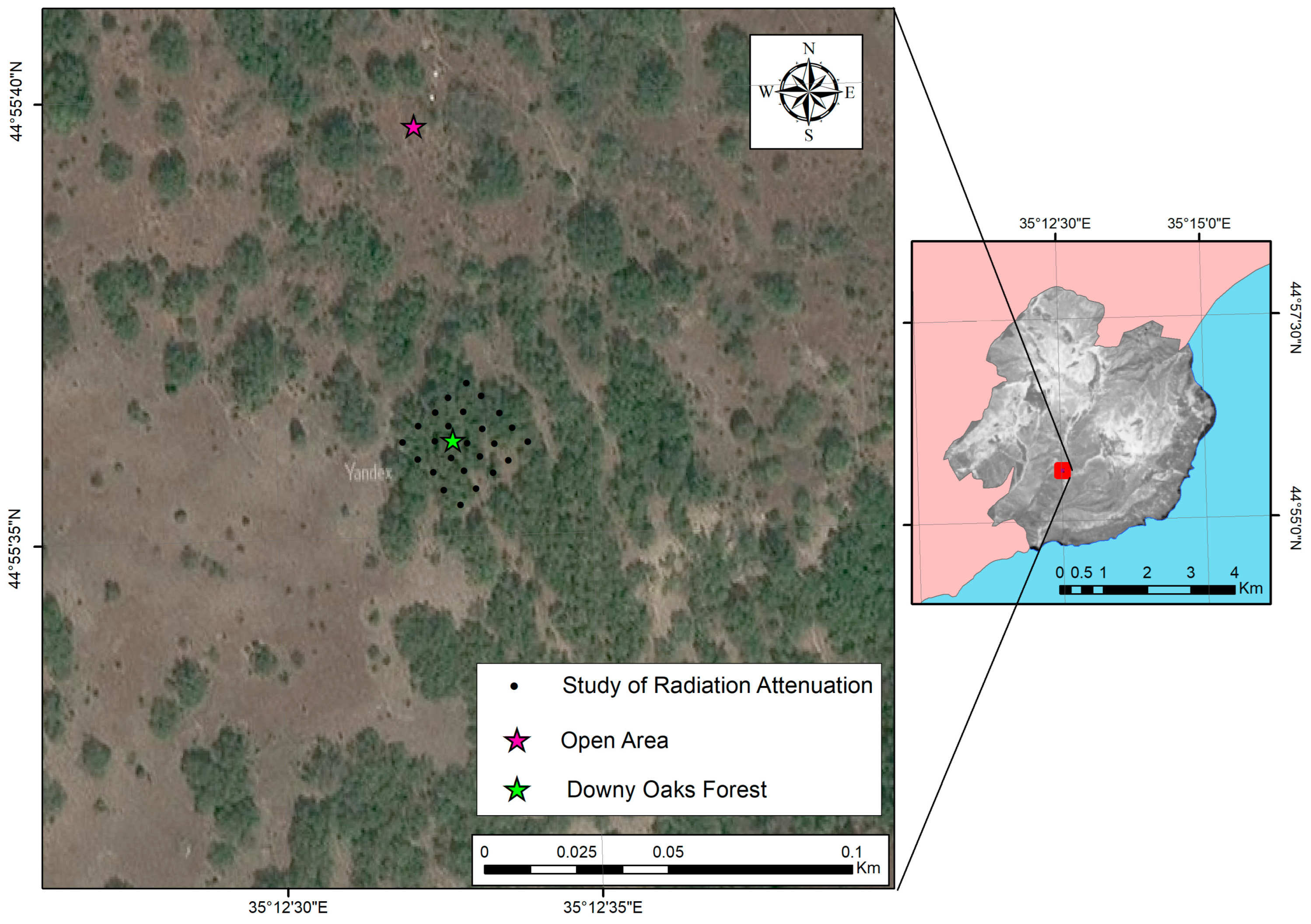
2.1. Study Area

In order to elucidate the intricacies of the heat balance and the distribution of heat fluxes within the forest landscapes of Southeastern Crimea [60], a key study site was selected, namely the downy oak forest, which represents a typical community type in this region. Situated within the territory of the Karadag Nature Reserve, this forest is located on the eastern-facing slope of the Besh-Tash ridge (Figure 1).
The investigated forest area occupies a gentle slope and is characterized by a single tree layer predominantly composed of downy oak (Quercus pubescens) and oriental hornbeam (Carpinus orientalis), with tree heights varying between 3.5 and 6 m. The area is also dotted with young oak saplings, reaching heights of up to 30 cm. The surveyed area constitutes a natural forest ecosystem characterized by an uneven distribution of herbaceous and shrubby vegetation. The trees in this area exhibit twisted trunks and wide canopies, with their leaves covered in fine, downy hairs. Employing rigorous phenological observations, it has been determined that the onset of foliar expansion in this ecosystem typically aligns with the latter stages of April. The downy oak forest is naturally renewable.
The adjacent open expanse, strategically situated within the habitat range of the Quercus pubescens (downy oak), showcases a contrasting botanical profile. The predominant ground cover in this context predominantly comprises mesophytic herbaceous species, with noteworthy representatives encompassing Teucrium chamaedrys, Aegonichon purpureo-caeruleum, Geum urbanium, and several others.

2.2. Research Methodology

For the research investigation, specific locations were carefully chosen to measure core meteorological parameters: an open area within the growth zone of the downy oak forest, where readings are collected without the influence of vegetative cover, and a typical forested site within the community, where parallel measurements are conducted to discern the effects of vegetation on the distribution of matter and energy fluxes.
The measurement of key meteorological parameters was carried out using the Davis Vantage Pro2 (Hayward, CA, USA) monitoring weather station installed in the open area, with hourly data acquisition. Based on these measurements, the incident solar radiation was quantified, and the fundamental components of the energy budget for the entire community were computed. To capture conditions beneath the forest canopy, TR series data loggers (Chelyabinsk, Russia) were strategically placed to record air temperature and humidity at heights of 0.5 m and 2 m above the soil surface, as well as at depths of 10 cm and 20 cm beneath the surface. Thus, to ensure the proper application of the methodology for computing the constituents of the thermal balance and to facilitate the comparability of results between an open area and a forested environment, measurement sensors were positioned at identical elevations.
To portray the condition of tree crowns and their radiation attenuation characteristics, measurements were conducted during various seasons, including the winter (leafless phase), the onset of spring (vegetation emergence), late spring, and the early half of summer (full crown development), under clear and calm weather conditions. These measurements were taken across a grid of points outlined in Figure 1. Utilizing this measurement grid, the extent of canopy closure and the penetration of solar radiation through tree canopies to the ground surface were determined. Subsequently, the obtained values were averaged to facilitate computational analysis and provide an encompassing description of the entire community.
The foundation of the heat balance equation lies in the principle of energy conservation, applied to a vertical column that encompasses the entirety of the external geographic envelope. The equation for the heat balance of the Earth’s surface is a summation of all heat fluxes transpiring between the surface and the surrounding space. Consequently, the equation assumes the following form:
R = LE + P + B,
where R—radiation balance, LE—signifies the heat dissipated through evaporation (L—representing latent heat of evaporation, E—the rate of evaporation or condensation), P—the turbulent heat flux, and B—flux into the soil.
Notably, the value of R is considered positive when it signifies heat inflow to the underlying surface, while all other variables are considered positive when they indicate heat outflow.
The methodology for calculating the radiation balance (R) is formulated based on the work of Budyko [1]:
R = (Q − q) − Ee,
where Q—total solar radiation;
q—reflected solar radiation;
Ee—effective emission.
The calculation of reflected solar radiation is carried out through the equation:
q = A·Q,
where A—albedo of the Earth’s surface.
The albedo, or the reflectivity, of the Earth’s surface is determined in accordance with the methodology outlined in [61]. The absorbed shortwave radiation is a result of the disparity between the total incoming radiation and the reflected radiation.
For the determination of the components within the longwave portion of the radiation balance, computations are executed based on the formulation attributed to D. Brunt [3].
The effective emission from the Earth’s surface is ascertained using the equation:
Ee = Es − δEa,
where Es—thermal radiation flux from the underlying surface directed towards the atmosphere;
Ea—atmospheric counter-radiation;
δ—relative emissivity of the surface.
The thermal radiation flux originating from the underlying surface is calculated using the equation:
Es = δσT4E,
where σ—Stefan–Boltzmann constant;
T—air temperature.
The counter-radiation emitted by the atmosphere is determined using the equation:
Ea = δσT4 (1 − a + b√e),
where a, b—empirical constants based on T. G. Beryland are utilized (a = 0.39, b = 0.058) [62];
e—partial pressure of water vapor.
The subsequent component of the energy budget involves the heat expenditure during evaporation, which is calculated as the product of latent heat of vaporization and the rate of evaporation. In natural conditions, the latent heat of vaporization remains relatively constant with respect to the temperature of the evaporating surface [1].
The latent heat of vaporization (L) is determined by the equation:
L = 597 − 0.6T,
where L—latent heat of vaporization (cal/g), T—temperature (°C).
The quantity of evaporation on the open site was measured using the sensor module of the Davis Vantage Pro2 weather station (Hayward, CA, USA). To estimate evaporation within the forested area, the following equation was employed [1]:
E = R B L + C p Q 1 Q 2 q 1 q 2 ,
where E—evaporation, R—radiation balance, B—heat flux into the soil, L—latent heat of vaporization, Cp—specific heat capacity of air under constant pressure [63], Q1 − Q2—indicates the temperature difference at two levels, q1 − q2—represents the difference in specific humidity at those levels.
The computation of soil heat flux is based on the temperature variation in the soil with respect to depth and time, considering known thermophysical characteristics.
B = C v τ S 1 ,
where CV—volumetric heat capacity; τ—time interval (in minutes) for which the average flux q1 is determined; S1—parameter indicating the change in temperature in the upper 20 cm soil layer during the interval τ. Value S1 is calculated using the equation:
S1 = S0 + S5 + S10 + S15 + S20,
where S0 = 20∙0.082 Δt0; S5 = 20∙0.333 Δt5; S10 = 20∙0.175 Δt10; S15 = 20∙0.156 Δt15; S20 = 20∙0.004 Δt20.
Here Δt0, Δt5, Δt10, Δt15 and Δt20 are the differences between corresponding soil temperature values in subsequent and previous observation periods. Δt0 corresponds to the temperature difference at the surface, and Δt5 is the difference at a depth of 5 cm, and so on.
The calculation of volumetric heat capacity is carried out using the method proposed by Makarychev and Mazirov [64]:
C V 0 = C w U s ( ρ 0 0.76 ρ w ) ρ 0 0.76 ρ w ,
where Cw = 4190/(kg·K) is the specific heat capacity of water, ρw = 1000 kg/m3 is water density, ρ0 represents the density of completely dry soil, and U signifies the soil moisture content.
U = P ρ ,
where P—porosity, ρ—density of the soil, g/cm3.
P = d ρ d ,
where d—density of the solid phase of the soil, g/cm3.
The volumetric heat capacity during the observation period is determined by the equation:
CV = CV0 + CwρwU,
where CV0—volumetric heat capacity of dry soil [65], CwρwU—heat capacity of the liquid present in the soil, U—soil moisture content.
The computation of turbulent heat flux is intricate, and often in climatological calculations involving terrestrial conditions, its values are derived from solving the heat balance equation. The simplest approach in this context involves determining heat exchange as the residual term in the balance equation, expressed as:
P = R − LE − B.

3. Results

3.1. Study Site: Open Area within the Downy Oak Forest Zone

The overall heat balance of a given territory hinges on its climatic parameters and the attributes of its underlying surface. A pivotal metric in this context is the radiation balance, which governs the distribution of heat fluxes and is a critical factor in shaping the ecosystem’s condition.

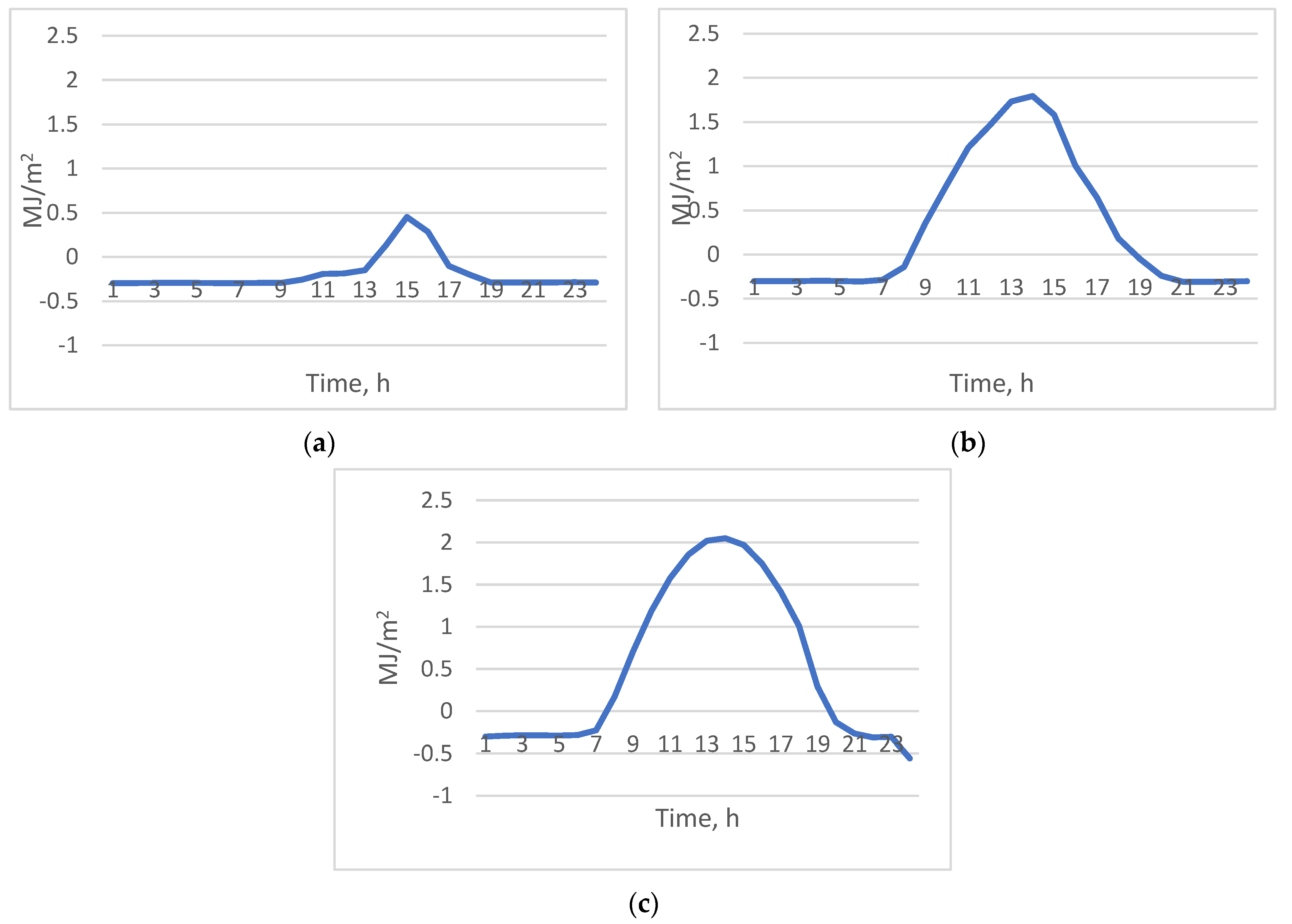
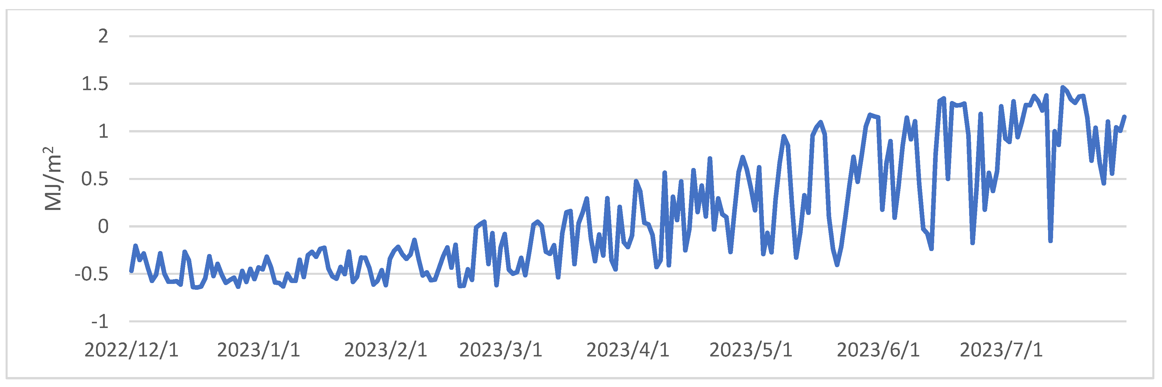
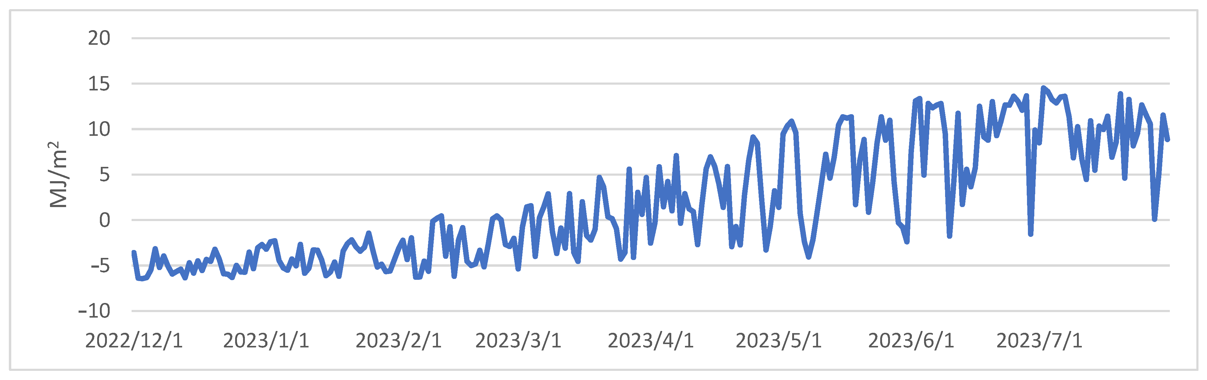
3.1.1. Radiation Balance Analysis

The obtained results shed light on the primary trends within the radiation balance and offer insights into its seasonal, monthly, and daily dynamics. Figure 2 depicts the daily averages of radiation balance recorded within the open area encompassed by the downy oak forest from 1 December 2022 to 31 July 2023.
As shown in Figure 2, a discernible pattern emerges from the progression of daily average radiation balance values spanning the period from 1 December 2022 to 31 July 2023. Analysis of the daily variations throughout the winter, spring, and summer seasons reveals that positive balance values are prevalent during daylight hours, whereas negative values dominate during nighttime (Figure 3). It is important to note that due to the reduced daylight hours and the lower solar angle during winter, minor positive balance values are confined to a short timeframe, occurring between 1 pm and 5 pm. With the lengthening of daylight hours and the higher solar position during spring, there is a noticeable upswing in both the magnitude of positive radiation balance values and their duration. In summer, the values exhibit further escalation, and their alterations manifest a smoother progression.
The heat balance encompasses the distribution of radiation balance values that govern the transfer of heat and energy within the ecosystem of the downy oak forest. Three primary energy transformation directions are distinguished: heat expenditure for evaporation, vertical turbulent heat exchange, and heat flux within the soil layer.

3.1.2. Evaporation Heat Expenditure

Explicit heat is allocated to the turbulent heat flux in the atmosphere and heat flux within the soil. The fraction of latent heat contributes to evaporation, equating to the product of latent heat of evaporation and the rate of evaporation. This latent heat is contingent upon the temperature of the evaporating surface [1]. The open area exhibits temporal variations in heat expenditure for evaporation (Figure 4).
Similar to radiation balance values, the distribution of heat expenditure for evaporation is nonuniform, gradually increasing during the spring period. In terms of percentage relation to radiation balance, heat expenditure for evaporation displays a highly heterogeneous nature, encompassing negative values signifying the reverse heat flux direction. In this context, heat expenditure for evaporation occurs during periods of negative radiation balance values at any time of day. Additionally, rare instances exhibit values ranging from 10% to 60% of the radiation balance value. Apart from these exceptions, the fraction of heat spent on evaporation rarely exceeds 1–5%.

3.1.3. Turbulent Heat Flux

Turbulent heat exchange between the underlying surface and the atmosphere is facilitated by the differential warming of the surface and its adjacent atmospheric layer. Its variations mirror those of the radiation balance and heat expenditure for evaporation, displaying nonuniform values with a prevailing upward trend (Figure 5).
In relation to radiation balance values, three distinct scenarios emerge. The first scenario witnesses negative turbulent flux values during positive radiation values, indicating cooling. This situation is prominent from late April to early May in the early morning. The second scenario involves significant turbulence exceeding radiation values by 120–300%, mainly observed during the first half of the day for negative fluxes directed towards cooling. Seasonal and diurnal patterns are not observed. These two situations are exceedingly rare, with the third scenario prevailing, where turbulent flux values account for around 90–100% of the radiation balance, signifying the primary energy expenditure direction within the landscape.

3.1.4. Soil Heat Flux

The soil heat flux characterizes changes in soil temperature with depth. In contrast to other components of the heat balance, it lacks an overall upward trend, displaying alternating heating and cooling of the soil layer (see Figure 6).
Contrary to the radiation balance, the soil heat flux assumes opposing values in the nighttime and early morning hours until noon during the winter period. In March, this time shifts to the early morning, accompanied by negative radiation values and positive soil heat flux, and vice versa during the daytime. A similar pattern is observed during the spring-summer period, although it remains more temporally stable. Soil heat flux values rarely exceed 40% of the radiation balance value, with their proportion typically not surpassing 10% in the majority of cases.

3.2. Study Site: Downy Oak Forest Zone

The aforementioned significances of heat balance components pertain to an open horizontal segment devoid of vegetative influence. The arboreal assemblage of downy oak forest within the focal site engenders a distinct canopy profile [66], which intercepts a quantum of incident solar radiation on its surface, allowing partial penetration into the sub-canopy domain. The extent of solar radiation permeation through the canopy is contingent on the cohesion and density of foliage, along with the presence of interstices amid the canopy. Deciduous arboreal species evince seasonal fluctuations in canopy foliation, extending to its abeyance throughout the winter interval. Consequently, three stages of canopy progression emerge over the observed period to expound on their states and nuances in radiation interception: the absence of foliage during winter, the onset of vernal growth, and the zenith of canopy expansion from late spring to the summer.
Of parallel note is the heterogeneous influx of solar radiation beneath the arboreal canopy, attributed to unconcealed canopy-lacking sectors and the spatiotemporal configuration of shading patterns. The quantum of incident solar radiation received by a specific point on the substrate is contingent on its azimuth relative to the solar rays’ orientation, i.e., predicated upon the gradient and aspect of the canopy contour. Nevertheless, in the comprehensive examination of the sylvan collective for radiation budget computation, averaged diurnal transmission values are enlisted.

3.2.1. Radiation Balance

During the winter span, the mean transmittance of solar radiation through the canopy averages 43.2%. This value is applicable across the entire winter epoch, extending until early May. Deliberating a level expanse within the winter forest on clear sunlit days yields transmittance levels reaching 90%. Nevertheless, these figures are a hypothetical construct, neglecting site-specific attributes. The survey locale is characterized by recurrent fog occurrences and wintry cloud cover. The terrain’s orography fosters shadow formation due to slopes, and select branches retain their foliage in discrete regions. These factors collectively influence the magnitude of solar radiation ingress beneath the canopy (Figure 7 and Figure 8).
The period of vegetative onset spans from March to April, with a canopy solar radiation transmittance value of 45.6% (Figure 9 and Figure 10). This value exceeds 50% for a broader time span; however, during the evening, due to elongated shadows caused by the slope, it significantly diminishes.
From May onward and throughout the summer season, the canopy maintains its full development state, permitting an average of only 19.1% solar radiation to pass through (Figure 11 and Figure 12). Elevated values are noted around midday, whereas at other times, transmittance values are below the mean.
This distribution of solar radiation between the sub-canopy space and the canopy surface determines the resultant sub-canopy balance values, wherein, with the process of tree canopy development nearing its zenith by late spring, radiation balance values sharply decline (Figure 13).
In the open area, all cumulative solar radiation is engaged in heat flux distribution, while within the forest community, it bifurcates into two zones: above the canopy and beneath the canopy, each independently shaping its own fluxes.

3.2.2. Evaporation Heat Expenditure

When considering heat expenditure values on evaporation beneath the canopy, negative values are observed, signifying condensation’s predominance over evaporation (Figure 14).
This is elucidated by the typical overcast weather and fog formation during the winter period. In the spring season, the considered indicator notably escalates.

3.2.3. Turbulent Heat Flux

Analogous to the open area, a comparable scenario is observed when examining the turbulent heat flux beneath the forest canopy. Negative turbulent flux values gradually increase through winter, peaking in April (Figure 15).

3.2.4. Turbulent Heat Flux

Similar to the open area, the soil heat flux is characterized by a uniform alternation of heating and cooling of the soil layer, encompassing the same range of values (Figure 16).
Despite the partial dataset, based on previously identified patterns, projections regarding the trajectory of heat balance element variations can be conjectured. Analogous to the open area, soil heat flux will maintain oscillations around zero, albeit with reduced amplitude during the summer. Simultaneously, heat expenditure on evaporation and turbulent heat flux exhibit similar patterns of change as the radiation balance, allowing for the anticipation of their gradual rise until May, followed by a rapid decline upon the canopy’s full development.

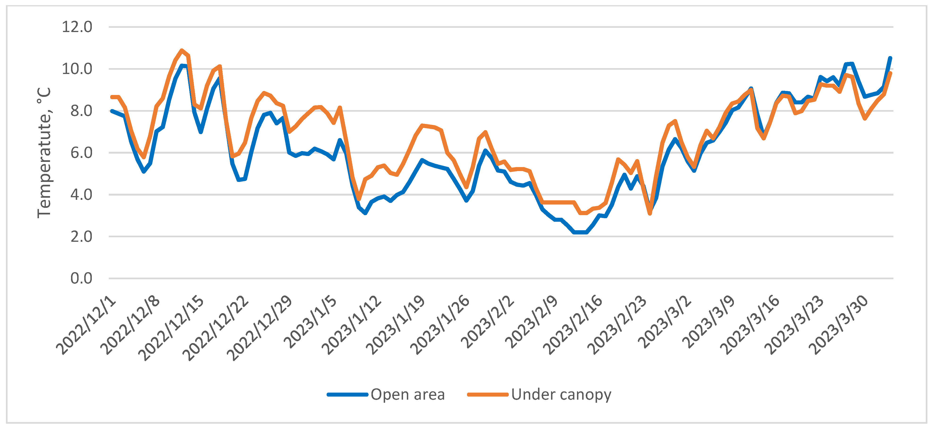
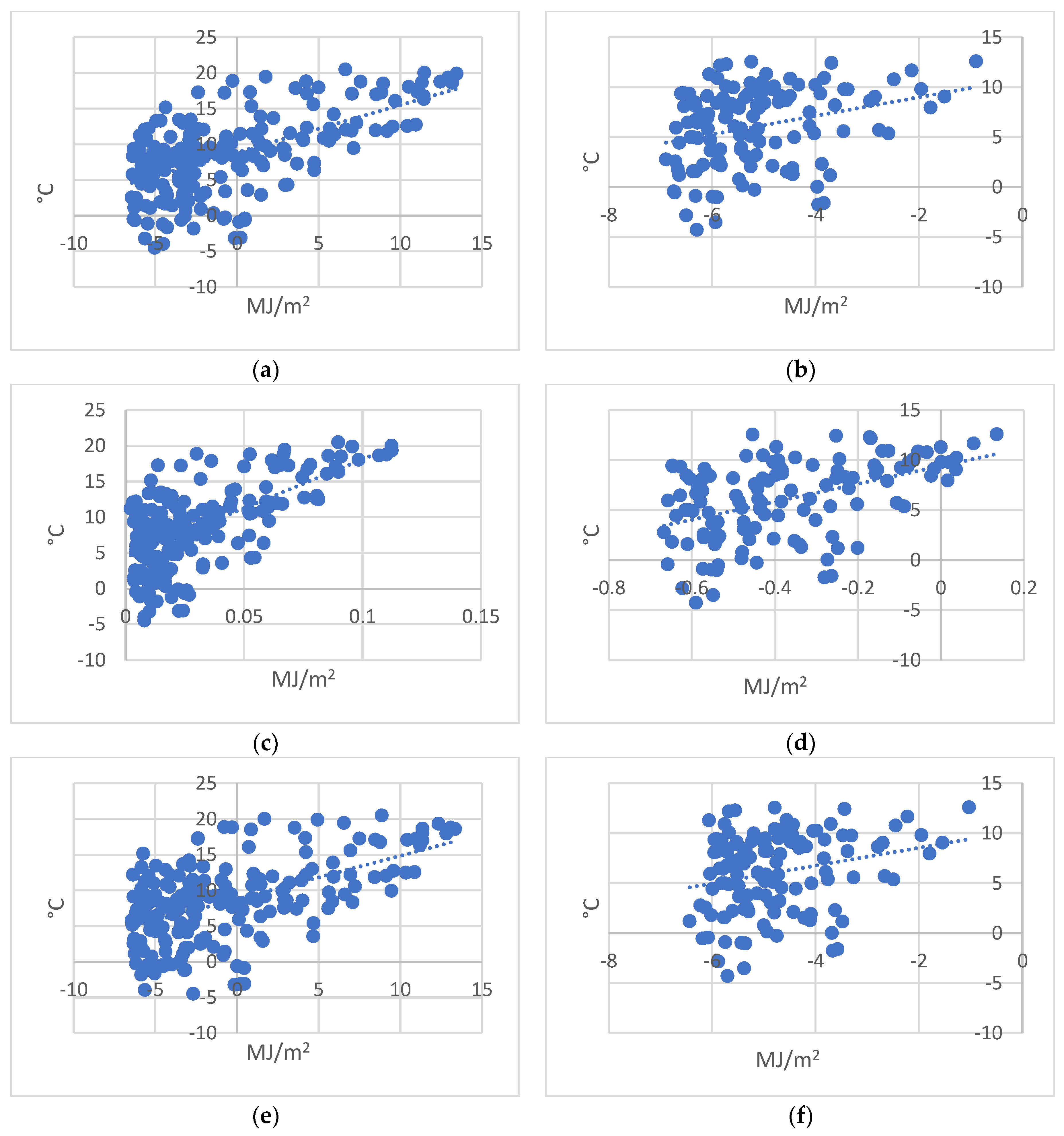
3.3. Air Temperature Relationship with Primary Heat Balance Elements

Furthermore, it is worth noting the alteration in the temperature profile, a fundamental heat characteristic, in both the open area and beneath the canopy. As depicted in Figure 17 and Figure 18, the average daily air temperature within the forest consistently surpasses that of the open area. The disparity is inconsequential during winter, but with the gradual expansion of the canopy, its influence on retaining heat in the sub-canopy space becomes more apparent. Similarly, during the summer, the situation is analogous due to the retention of daytime accumulated heat during the night and early morning, in contrast to the open area.
With a more detailed scrutiny of temperature changes encompassing diurnal values, during winter, the temperature surplus within the forest amounts to approximately 0.1 °C. During midday, this surplus could range from 0.7 °C to 6 °C in isolated hours. In March, the nocturnal difference ranges from 0.1 °C to 0.5 °C, and between 8 and 15 h, the difference can reach 3 °C, while at midday, the maximum difference extends to 10 °C. During the spring and summer period, hourly differences could also attain 4–10 °C. The air temperature exceeding that of the open area is documented throughout the observed period, with differences typically not exceeding 1 °C during the nighttime and early morning.
The average daily soil temperature values demonstrate the persistence of heat retention beneath the forest canopy during the winter period. By March, these values reach a state of equilibrium, and as the vegetative phase commences, a discernible reduction in temperature within the forested domain becomes apparent (Figure 19 and Figure 20).
The differential analysis of soil temperature between the open area and the forested environment manifests a relatively uniform pattern in contrast to air temperature values, exhibiting a less pronounced abruptness. Through the winter and spring intervals, the average disparity approximates 1 °C, occasionally peaking at 2.7 °C. In select instances, during the nocturnal hours, the open area’s temperature might modestly exceed the forest’s by approximately 0.2 °C.
Throughout the summer phase, within the canopy’s shaded precincts, soil temperature recedes and reveals nocturnal deviations of 2–3 °C relative to the open area. By day, this discrepancy can further extend to 7–8 °C.
When scrutinizing the intricate relationship between air temperature and primary heat balance parameters, a consistent trend emerges wherein heightened temperature aligns with augmented radiation balance, heat consumption due to evaporation, and turbulent exchange (Figure 21). However, this trend is not mirrored in the context of soil heat flux.
Despite the overarching regularity in value distribution observed across the open area and the expanse of the downy oak forest, a distinctive phenomenon emerges within the forested environment. Within this ecological context, the interplay between air temperature and the fundamental constituents of heat balance undergoes a pronounced attenuation in comparison to the conditions evident in the open area. This specific observation accentuates a conspicuously less robust relationship between air temperature and the essential components of heat balance within the forested milieu. Consequently, this accentuation further underscores the manifestation of a more intricate organizational structure inherent to the examined ecosystem, accompanied by the intricate pattern of heat and energy flux distribution within its enclosed boundaries.

4. Discussion

Thus, the analysis of the research findings unequivocally underscores the pivotal role of vegetative cover in modulating the dispersion dynamics of incident solar radiation within the precincts of a forest ecosystem. This impact is most pronounced in deciduous arboreal domains, where the cyclic alternation of crown states during the course of the seasons assumes a preeminent function in configuring the microclimatic conditions.
Delving into the radiation balance metrics of exposed terrain and the sylvan canopy region brings into sharp relief the conspicuous imprint of the vegetal mantle. In this context, three discernible epochs, characterized by varying degrees of influence, are manifestly demarcated (Figure 22).
These demarcated epochs conspicuously align with the arboreal foliage cycle: the apogee of radiation impact and balance transpires during the season of denuded winter tide, a more appreciable influence takes root during the nascent phases of vernal vegetation, and the period with the most significant influence occurs with the maximum development of the crown from late spring to mid-autumn. Analogously, a gradual attenuation of this influence in the autumnal interval, concomitant with foliar abscission, is rendered plausible.
In accordance with the change of seasons and changes in the vegetation stage, the radiation balance, in turn, forms the main heat fluxes in the ecosystem. Consistent with the ascertained regularity governing the temporal change of heat dissipation due to evapotranspiration and turbulent heat flux, these transmutations mirror the radiation balance and undergo an incremental augmentation until the onset of full canopy development in spring. After that, these parameters decrease, in contrast to the values of the open area, where there is a constant increase.
A pertinent consideration pertains to the subsurface heat flux. While alternating increments and decrements in magnitudes characterize both underpinning domains, the arboreal foliage serves to ameliorate fluctuations and curtail the amplitude of perturbations in this parametric continuum.
Hence, the present study pioneers the calculation of heat balance parameters at a local stratum predicated upon hourly surveillance, thereby affording a finer-grained exposition of the temporal modulations inherent to individual parameters. This deviates from prevailing works, which predominantly engage in an examination of heat balance across monthly and seasonal intervals, thereby underscoring the precision underpinning the endeavor.
The notable ramifications of canopy configurations on the realignment of key meteorological attributes are readily manifest. Noteworthy parallels are evident in kindred investigations, such as those conducted by Ohta et al. [54], which scrutinize the ramifications of arboreal canopies on snowmelt kinetics across open terrain and sylvan expanses. Evidently, concurrence can be reached with the observations of Haag, R.W. and Bliss, L.C. [35], who highlight the accentuation of soil heat flux and soil temperature consequent to the attenuation of vegetative coverage.
Conversely, the datasets cataloged within reanalysis repositories and antecedent scholarly undertakings [67,68,69] evince a coarse-grained spatial resolution, precluding their application in the discernment of localized spatiotemporal patterns. For instance, the resolutions afforded by ERA5 [67] amount to 11,132 m/pixel, whereas GLDAS-2.1 [68] presents a resolution of 27,830 m/pixel. Therefore, a continuous amelioration of existing datasets remains imperative. It is self-evident that the dataset procured, being intrinsically most veracious for the purviewed locale, may be prospectively harnessed across diverse investigatory paradigms.
Evidently, the complexities intrinsic to the study of heat balance within sylvan ecosystems at a localized scale are principally tethered to the requisites of highly precise and relatively extravagant instrumentation that automatically captures cardinal meteorological attributes. Absent this, substantial manual exertions and temporal investments are necessitated for data collection and subsequent manual analyses conducted at 1-min or hourly cadences. The imperative of automated acquisition of meteorological attributes concomitant with the operational dynamics of forest ecosystems scarcely warrants dispute. Nonetheless, the utilization of autonomous weather stations introduces certain exigencies, primarily on account of the periodicity entailed in data compilation and the operational resilience of receivers subjected to temperature fluctuations. Furthermore, the constrained energy reservoir of battery arrays represents a salient limitation. In the event of battery failure underpinning console-receiver functionality, the prospect of data loss during observation is ineluctable. Simultaneously, environmental imperatives demand circumspect battery disposal practices.
A salient avenue for future exploration resides in the juxtaposition of the procured solar radiation transmittance metrics, heat balance elements, and the projected canopy’s influence with the computation of the Leaf Area Index. Moreover, prospective lines of inquiry affiliated with the exploration of radiation and heat balance within forested realms could encompass the scrutiny of the carbon cycle, prognostications germane to climate alterations, sylvicultural stewardship, and the expansion of monitoring gridworks. Additionally, the extrapolation of the acquired data, coupled with the explication of patterns and linkages with remote sensing and spaceborne acquisitions in the context of modeling heat and energetic fluxes, assumes an auspicious investigative trajectory.

5. Conclusions

As a result of the studies carried out, general information on the seasonal and daily dynamics of the components of the heat balance in the downy oak forest on the territory of the landscape-ecological station was obtained. The various constituents of the heat balance, encompassing the radiation balance, heat dissipation due to evaporation, turbulent heat exchange prevailing within the atmosphere, and the subterranean heat flux, have been meticulously computed for the timeframe spanning 1 December 2022 to 31 July 2023. Primary data have been amassed, elucidating the discernible patterns governing the distribution of radiation balance into discernable heat and energy fluxes across the expanse of feather-grass oak landscapes located in Southeastern Crimea.
Evidently, the preponderance of the radiation balances are allocated towards the perturbations engendered by turbulent heat flux, with a comparably minor allotment attributed to processes involving evaporation and the subsurface heat flux. Intriguingly, a temporal delineation of the total solar radiation permeating the sub-canopy region during the diurnal phase has been discerned, contingent upon the seasonal progression and the state of the crown foliage.
The main elements of the heat balance have been calculated for two key areas: the open area and the downy oak forest itself. Notably, the modulations exhibited by turbulent heat flux and heat dissipation due to evaporation mirror the oscillations inherent to radiation balance values, characterized by a gradual ascension from the winter period culminating in the summer season. Conversely, the heat flux penetrating the substratum demonstrates a recurrent alternation of escalation and abatement within a defined spectrum, accompanied by a dampening of amplitude during the zenith of the summer phase.
The features of air and soil temperature changes in the open area and under the forest canopy by season are considered. It has been identified that the average daily air temperature within the forest during the studied period consistently surpasses the temperature in the open area. This is attributable to the presence of the canopy, and its influence becomes more pronounced as it develops. Regarding soil temperature values, it is noteworthy that heat retention beneath the canopy persists during the winter period, with values stabilizing in March. As the vegetation period commences in the forested area, a decline in temperature becomes evident.
The correlation between temperature parameters and constituents of the heat balance has been ascertained. It has been conclusively posited that the arboreal verdure invariably exercises an indelible influence upon the ecosystem’s heat balance. However, the extent of its influence is inexorably contingent upon the cyclical transition of foliage among the arboreal populace. As an overarching principle, the profundity of the canopy’s developmental status directly engenders a commensurate impact upon the distributional patterning of heat and energetic fluxes.

Author Contributions

Conceptualization, R.G.; methodology, R.G. and M.S.; validation, M.S., V.T. and T.G.; formal analysis, M.S. and V.T.; investigation, M.S.; resources, M.S., V.T. and T.G.; data curation, M.S. and T.G.; writing—original draft preparation, R.G., M.S., V.T. and T.G.; writing—review and editing, R.G., M.S., V.T. and T.G.; visualization, M.S., V.T. and T.G.; supervision, R.G.; project administration, R.G. All authors have read and agreed to the published version of the manuscript.

Funding

This research was funded by Russian Science Foundation, grant number 22-27-00579.

Data Availability Statement

Not applicable.

Conflicts of Interest

The authors declare no conflict of interest. The funders had no role in the design of the study, in the collection, analyses, or interpretation of data, in the writing of the manuscript, or in the decision to publish the results.

References

  1. Budyko, M.I. Energy Budget of the Earth’s Surface; Gidrometeoizdat: Leningrad, Russia, 1956; 286p. [Google Scholar]
  2. Ippolitov, I.I.; Kabanov, M.V.; Loginov, S.V.; Sokolov, K.I.; Kharyutkina, E.V. Variability of components of the surface thermal balance at the Asian Russia area during the current global warming. Opt. Atmos. Okeana 2011, 24, 22–29. [Google Scholar]
  3. Brunt, D. Notes on radiation in the atmosphere. I. Q. J. R. Meteorol. Soc. 1932, 58, 389–420. [Google Scholar] [CrossRef]
  4. Christen, A.; Novak, M.D.; Black, A.T.; Brown, M. The Budget of Turbulent Kinetic Energy within and Above a Sparse Lodgepole Pine Stand. Available online: https://www.researchgate.net/publication/51995947_The_budget_of_turbulent_kinetic_energy_within_and_above_a_sparse_Lodgepole_Pine_stand (accessed on 8 August 2023).
  5. Njuki, S.M.; Mannaerts, C.M.; Su, Z. Accounting for Turbulence-Induced Canopy Heat Transfer in the Simulation of Sensible Heat Flux in SEBS Model. Remote Sens. 2023, 15, 1578. [Google Scholar] [CrossRef]
  6. Vecellio, D.J.; Wolf, S.T.; Cottle, R.M.; Kenney, W.L. Utility of the Heat Index in defining the upper limits of thermal balance during light physical activity (PSU HEAT Project). Int. J. Biometeorol. 2022, 66, 1759–1769. [Google Scholar] [CrossRef]
  7. Wang, J.; Buttar, N.A.; Hu, Y.; Lakhiar, I.A.; Javed, Q.; Shabbir, A. Estimation of Sensible and Latent Heat Fluxes Using Surface Renewal Method: Case Study of a Tea Plantation. Agronomy 2021, 11, 179. [Google Scholar] [CrossRef]
  8. Fuchs, S.; Beardsmore, G.; Chiozzi, P.; Espinoza-Ojeda, O.M.; Gola, G.; Gosnold, W.; Harris, R.; Jennings, S.; Liu, S.; Negrete-Aranda, R.; et al. A new database structure for the IHFC Global Heat Flow Database. Int. J. Terr. Heat Flow Appl. 2021, 4, 1–14. [Google Scholar] [CrossRef]
  9. Bhattacharya, B.K.; Mallick, K.; Desai, D.; Bhat, G.S.; Morrison, R.; Clevery, J.R.; Woodgate, W.; Beringer, J.; Cawse-Nicholson, K.; Ma, S.; et al. A coupled ground heat flux–surface energy balance model of evaporation using thermal remote sensing observations. Biogeosciences 2022, 19, 5521–5551. [Google Scholar] [CrossRef]
  10. Ander, T. Earth’s Balanced Climates in View of Their Energy Budgets. Available online: https://doi.org/10.21203/rs.3.rs-568771/v1 (accessed on 8 August 2023).
  11. Liang, S.; Wang, D.; He, T.; Yu, Y. Remote sensing of earth’s energy budget: Synthesis and review. Int. J. Digit. Earth 2018, 12, 737–780. [Google Scholar] [CrossRef]
  12. Voeykov, V.A. Klimaty Zemnogo Shara, v Osobennosti Rossii [Climates of the Globe, Especially Russia]; A. Ilyin: St. Petersburg, FL, USA, 1884. [Google Scholar]
  13. Berlyand, T.G. Radiation and heat balance of the European territory of the USSR. Proc. Voeikov Main Geophys. Obs. 1948, 10, 72. [Google Scholar]
  14. Alestalo, M. The energy budget of the earth–atmosphere system in Europe. Tellus A Dyn. Meteorol. Oceanogr. 1981, 33, 360. [Google Scholar] [CrossRef]
  15. Killeen, T.; Burns, A.; Azeem, I.; Cochran, S.; Roble, R. A theoretical analysis of the energy budget in the lower thermosphere. J. Atmos. Solar Terr. Phys. 1997, 59, 675–689. [Google Scholar] [CrossRef]
  16. Mannstein, H. Surface Energy Budget, Surface Temperature and Thermal Inertia. In Remote Sensing Applications in Meteorology and Climatology; Springer: Dordrecht, The Netherlands, 1987; pp. 391–410. [Google Scholar] [CrossRef]
  17. Zeman, O.; Tennekes, H. Parameterization of the Turbulent Energy Budget at the Top of the Daytime Atmospheric Boundary Layer. J. Atmos. Sci. 1977, 34, 111–123. [Google Scholar] [CrossRef]
  18. Pavlov, A.V. Thermal Physics of Landscapes Science; Nayka: Novosibirsk, Russia, 1979; 284p. [Google Scholar]
  19. Isakov, A.L.; Lavrova, A.Y. Solar radiation and temperature regime of the roadbed. Path Track Manag. 2016, 3, 15–19. [Google Scholar]
  20. Prokhorova, U.; Terekhov, A.; Ivanov, B.; Verkulich, S. Calculation of the Heat Balance Components of the Aldegonda Glacier (Western Spitsbergen) During the Ablation Period according to the Observations of 2019. Kriosf. Zemli 2021, 25, 50–60. [Google Scholar] [CrossRef]
  21. Trenberth, K.E.; Fasullo, J.T.; Kiehl, J. Earth’s Global Energy Budget. Bull. Am. Meteorol. Soc. 2009, 90, 311–324. [Google Scholar] [CrossRef]
  22. Kiehl, J.T.; Trenberth, K.E. Earth’s Annual Global Mean Energy Budget. Bull. Am. Meteorol. Soc. 1997, 78, 197–208. [Google Scholar] [CrossRef]
  23. Loeb, N.G.; Wielicki, B.A.; Doelling, D.R.; Smith, G.L.; Keyes, D.F.; Kato, S.; Manalo-Smith, N.; Wong, T. Toward Optimal Closure of the Earth’s Top-of-Atmosphere Radiation Budget. J. Clim. 2009, 22, 748–766. [Google Scholar] [CrossRef]
  24. Wang, Q.; Zhang, H.; Yang, S.; Chen, Q.; Zhou, X.; Xie, B.; Wang, Y.; Shi, G.; Wild, M. An assessment of land energy balance over East Asia from multiple lines of evidence and the roles of the Tibet Plateau, aerosols, and clouds. Atmos. Meas. Tech. 2022, 22, 15867–15886. [Google Scholar] [CrossRef]
  25. Savijärvi, H. The atmospheric energy budgets over North America, the North Atlantic and Europe based on ECMWF analyses and forecasts. Tellus A Dyn. Meteorol. Oceanogr. 1983, 35, 39. [Google Scholar] [CrossRef]
  26. Shongwe, M.E.; Graversen, R.G.; van Oldenborgh, G.J.; van der Hurk, B.J.J.M.; Doblas-Reyes, F.J. Energy budget of the extreme Autumn 2006 in Europe. Clim. Dyn. 2009, 36, 1055–1066. [Google Scholar] [CrossRef]
  27. Hagemann, S.; Machenhauer, B.; Jones, R.; Christensen, O.B.; Jacob, D.; Vidale, P.L.; Déqué, M. Evaluation of water and energy budgets in regional climate models applied over Europe. Clim. Dyn. 2004, 23, 547–567. [Google Scholar] [CrossRef]
  28. Partington, J.R. An Advanced Treatise on Physical Chemistry. Available online: https://archive.org/details/advancedtreatise0003jrpa/page/n5/mode/2up (accessed on 8 August 2023).
  29. Prigogine, I.; Defay, R. Chemical Thermodynamics; Longmans, Green & Co.: London, UK, 1954. [Google Scholar]
  30. Adkins, C.J. Balance Thermodynamics. Available online: https://archive.org/details/equilibriumtherm0000adki (accessed on 8 August 2023).
  31. Landsberg, P.T. Thermodynamics and Statistical Mechanics; Oxford University Press: Oxford, UK, 1978; p. 11. [Google Scholar]
  32. Gerasimov, Y.I. (Ed.) Course of Physical Chemistry; Khimia: Moscow, Russia, 1969. [Google Scholar]
  33. Perrot, P. A to Z of Thermodynamics; Oxford University Press: Oxford, UK, 1998. [Google Scholar]
  34. Clark, J.O.E. The Essential Dictionary of Science. Available online: https://archive.org/details/essentialdiction0000unse (accessed on 8 August 2023).
  35. Haag, R.W.; Bliss, L.C. Functional Effects of Vegetation on the Radiant Energy Budget of Boreal Forest. Can. Geotech. J. 1974, 11, 374–379. [Google Scholar] [CrossRef]
  36. Surova, N.A. Productivity and Heat Balance of Boreal Forests in South-Kuril Islands. Samara Luka 2018, 27, 147–160. [Google Scholar]
  37. Bityukov, N.A. Heat Exchange and Heat Balance of Brown Forest Soils under Beech Tree Forest. Bull. Sochi State Univ. 2012, 3, 224–230. [Google Scholar]
  38. Akimova, D.P. Radiation and thermal regimes in oak-pine crops at an altitude of 1300 m and in the field of nutrition of mineral sources. Sci. Work. All Russ. Sci. Res. Inst. For. For. Mech. 1972, 11, 3–11. [Google Scholar]
  39. Alekseev, V.A. Light Mode of the Forest; Gidrometeoizdat: Leningrad, Russia, 1975; 227p. [Google Scholar]
  40. Vygodskaya, N.N. Radiation regime of 30-year-old oak forest in daily and seasonal dynamics. In Light Regime, Photosynthesis and Forest Productivity; Nauka: Moscow, Russia, 1967; pp. 77–94. [Google Scholar]
  41. Vygodskaya, N.N. Methodology of phytoactinometric studies in mountainous areas. In Phytoactinometric Studies of Mountain Forests; USSR Academy of Sciences: Vladivostok, Russia, 1977; pp. 20–37. [Google Scholar]
  42. Zukert, N.V.; Vygodskaya, N.N.; Lebedeva, M.G.; Sherman, E.V. Radiation regime under the canopy of mountain forests. In Phytoactinometric Studies of Mountain Forests; USSR Academy of Sciences: Vladivostok, Russia, 1967; pp. 162–178. [Google Scholar]
  43. Ugarov, I.S. The radiation budget of a forest in Central Yakutia. Sci. Alm. 2018, 9, 128–133. [Google Scholar]
  44. Stewart, J.; Thom, A. Energy budgets in pine forest. Q. J. R. Meteorol. Soc. 1973, 99, 154–170. [Google Scholar] [CrossRef]
  45. Thom, A.; Stewart, J.; Oliver, H.; Gash, J. Comparison of aerodynamic and energy budget estimates of fluxes over a pine forest. Q. J. R. Meteorol. Soc. 1975, 101, 93–105. [Google Scholar] [CrossRef]
  46. Nousu, J.P.; Lafaysse, M.; Mazzotti, G.; Ala-aho, P.; Marttila, H.; Cluzet, B.; Aurela, M.; Lohila, A.; Kolari, P.; Boone, A.; et al. Modelling snowpack dynamics and surface energy budget in boreal and subarctic peatlands and forests. EGUsphere 2023, 2023, 1–52. [Google Scholar]
  47. Reimer, A.; Desmarais, R. Micrometeorological energy budget methods and apparent diffusivity for Boreal forest and grass sites at Pinawa, Manitoba, Canada. Agric. Meteorol. 1973, 11, 419–436. [Google Scholar] [CrossRef]
  48. Constantin, J.; Inclan, M.; Raschendorfer, M. The energy budget of a spruce forest: Field measurements and comparison with the forest–land–atmosphere model (FLAME). J. Hydrol. 1998, 212–213, 22–35. [Google Scholar] [CrossRef]
  49. Wu, J.; Guan, D.; Han, S.; Shi, T.; Jin, C.; Pei, T.; Yu, G. Energy budget above a temperate mixed forest in northeastern China. Hydrol. Process. 2006, 21, 2425–2434. [Google Scholar] [CrossRef]
  50. Lindroth, A.; Iritz, Z. Surface energy budget dynamics of short-rotation willow forest. Theor. Appl. Clim. 1993, 47, 175–185. [Google Scholar] [CrossRef]
  51. Storr, D.; Tomlain, J.; Cork, H.F.; Munn, R.E. An Energy Budget Study Above the Forest Canopy at Marmot Creek, Alberta, 1967. Water Resour. Res. 1970, 6, 705–716. [Google Scholar] [CrossRef]
  52. Tunick, A. A radiation and energy budget algorithm for forest canopies. Meteorol. Atmos. Phys. 2005, 91, 237–246. [Google Scholar] [CrossRef]
  53. Vourlitis, G.L.; Nogueira, J.D.S.; Lobo, F.D.A.; Sendall, K.M.; de Paulo, S.R.; Dias, C.A.A.; Pinto, O.B.; de Andrade, N.L.R. Energy balance and canopy conductance of a tropical semi-deciduous forest of the southern Amazon Basin. Water Resour. Res. 2008, 44, W03412. [Google Scholar] [CrossRef]
  54. Ohta, T.; Hashimoto, T.; Ishibashi, H. Energy budget comparison of snowmelt rates in a deciduous forest and an open site. Ann. Glaciol. 1993, 18, 53–59. [Google Scholar] [CrossRef]
  55. Ved’, I.P. Peculiarities of energy budget and radiation balance of pine plantations under frost conditions. Izv. USSR Acad. Sci. Geogr. 1969, 4, 109–113. [Google Scholar]
  56. Ved’, I.P. The Radiation Balance and the Phytoclimate of Young Stands of Pinus Pallasiana Lamb. Lesovedeniye 1974, 5, 3–9. [Google Scholar]
  57. Ved’, I.P. Energy budget and radiation balance of the forest in the Crimean Highlands. Izv. USSR Acad. Sci. Geogr. 1971, 2, 61–70. [Google Scholar]
  58. Bokov, V.A. (Ed.) Landscape and Geophysical Conditions for the Growth of Forests in the Southeastern Part of the Mountainous Crimea; Tavria-Plus: Simferopol, Ukraine, 2001. [Google Scholar]
  59. Li, Z.; Deng, X.; Shi, Q.; Ke, X.; Liu, Y. Modeling the Impacts of Boreal Deforestation on the Near-Surface Temperature in European Russia. Adv. Meteorol. 2013, 2013, 486962. [Google Scholar] [CrossRef]
  60. Gorbunov, R.; Tabunshchik, V.; Gorbunova, T.; Safonova, M. Water Balance Components of Sub-Mediterranean Downy Oak Landscapes of Southeastern Crimea. Forests 2022, 13, 1370. [Google Scholar] [CrossRef]
  61. Rakhmanov, V.V. The Hydroclimatic Role of Forests; Lesnaya Promyshlennost’: Moscow, Russia, 1984; 240p. [Google Scholar]
  62. Berlyand, M.E. Prediction and Regulation of the Thermal Regime of the Surface Layer of the Atmosphere; Gidrometeoizdat: Leningrad, Russia, 1956; 435p. [Google Scholar]
  63. Air Density, Its Specific Heat Capacity, Viscosity and Other Physical Properties. Available online: http://thermalinfo.ru/svojstva-gazov/gazovye-smesi/fizicheskie-svojstva-vozduha-plotnost-vyazkost-teploemkost-entropiya (accessed on 8 August 2023).
  64. Makarychev, S.V.; Mazirov, M.A. Thermophysical Foundations of Soil Reclamation; All-Russian Scientific Research Institute of Agrochemistry named after D.N. Pryanishnikov: Moscow, Russia, 2004; 290p. [Google Scholar]
  65. Makarychev, S.V. The Ability to Determine the Dimensional Heat Capacity of Soils. RU Patent No. 4914260, 20 November 1993. 4p. [Google Scholar]
  66. Gorbunov, R.V.; Gorbunova, T.Y.u.; Kuznetsov, A.N.; Kuznetsova, S.P.; Lebedev Ya, O.; Nguen, D.H.; Vu, M. Peculiarities of Formation of Radiation Balance Elements in the Mid-Mountain Tropical Forests of Southern Vietnam. Proc. T.I.Vyazemsky Karadag Sci. Stn. Nat. Reserve Russ. Acad. Sci. USA 2019, 4, 3–16. [Google Scholar] [CrossRef]
  67. Muñoz Sabater, J. ERA5-Land Monthly Averaged Data from 1981 to Present. Copernicus Climate Change Service (C3S) Climate Data Store (CDS). Available online: https://cds.climate.copernicus.eu/cdsapp#!/dataset/10.24381/cds.68d2bb30?tab=overview (accessed on 8 August 2023).
  68. Wang, Y.; Zhao, X.; Mamtimin, A.; Sayit, H.; Abulizi, S.; Maturdi, A.; Yang, F.; Huo, W.; Zhou, C.; Yang, X.; et al. Evaluation of Reanalysis Datasets for Solar Radiation with In Situ Observations at a Location over the Gobi Region of Xinjiang, China. Remote Sens. 2021, 13, 4191. [Google Scholar] [CrossRef]
  69. Jiang, H.; Yang, Y.; Wang, H.; Bai, Y.; Bai, Y. Surface Diffuse Solar Radiation Determined by Reanalysis and Satellite over East Asia: Evaluation and Comparison. Remote Sens. 2020, 12, 1387. [Google Scholar] [CrossRef]
Figure 1. Location of the key study site in the downy oak forest within the Karadag Nature Reserve.
Forests 14 01927 g001
Figure 2. Daily average radiation balance values within the open area of the downy oak forest zone during the study period.
Forests 14 01927 g002
Figure 3. Radiation balance in: (a)—winter (17 January), (b)—spring (15 April), (c)—summer (6 June).
Forests 14 01927 g003
Figure 4. Daily heat expenditure for evaporation within the open area during the study period.
Forests 14 01927 g004
Figure 5. Turbulent heat flux within the open area during the study period.
Forests 14 01927 g005
Figure 6. Daily soil heat flux within the pen area during the study period.
Forests 14 01927 g006
Figure 7. Distribution of total solar radiation during the leafless period.
Forests 14 01927 g007
Figure 8. Distribution of reflected solar radiation during the leafless period.
Forests 14 01927 g008
Figure 9. Distribution of total solar radiation during the vegetative onset period.
Forests 14 01927 g009
Figure 10. Distribution of reflected solar radiation during the vegetative onset period.
Forests 14 01927 g010
Figure 11. Distribution of total solar radiation during the full vegetation period.
Forests 14 01927 g011
Figure 12. Distribution of reflected solar radiation during the full vegetation period.
Forests 14 01927 g012
Figure 13. Average daily radiation balance values under the canopy during the study period.
Forests 14 01927 g013
Figure 14. Heat Expenditure on evaporation under the canopy.
Forests 14 01927 g014
Figure 15. Turbulent heat flux under the canopy.
Forests 14 01927 g015
Figure 16. Soil heat flux under the canopy.
Forests 14 01927 g016
Figure 17. Air temperature in the open area and under the canopy of the downy oak forest.
Forests 14 01927 g017
Figure 18. Temperature difference between the open area and under the canopy of the downy oak forest.
Forests 14 01927 g018
Figure 19. Soil temperature in the open area and under the canopy of the downy oak forest.
Forests 14 01927 g019
Figure 20. Soil temperature differential between the downy oak forest canopy and the open area.
Forests 14 01927 g020
Figure 21. Relationship between air temperature and: radiation balance in the open area (a) and under the canopy (b), Heat Expenditure on Evaporation in the Open Area (c) and under the canopy (d), Turbulent Heat Flux in the Open Area (e) and under the canopy (f).
Forests 14 01927 g021
Figure 22. Difference in radiation balance values between an open area and under the forest canopy.
Forests 14 01927 g022
Disclaimer/Publisher’s Note: The statements, opinions and data contained in all publications are solely those of the individual author(s) and contributor(s) and not of MDPI and/or the editor(s). MDPI and/or the editor(s) disclaim responsibility for any injury to people or property resulting from any ideas, methods, instructions or products referred to in the content.

