Abstract
Vertical vegetation differentiation is the most important form of spatial pattern in mountainous areas. It is of great significance to accurately divide vegetation into vertical zones for the study of mountain ecosystems and ecological protection. In order to accurately divide the vertical zone of mountain vegetation and determine the spatial distribution of mountain vegetation, the relationship between the vegetation index of various vegetation types and altitude was examined using remote sensing and geographic information technology. Taking Taibai Mountain, the main peak of the Qinling Mountains in China, as the study area, based on the difference in NDVI between summer and autumn (DNSA), this work constructed a DEM-NDVI scatter plot and quantified the boundary of the vertical zone by the half-peak width calculation method. The findings showed that: (1) the vertical distribution pattern of mountain vegetation may very well be reflected in the scatterplot that NDSA and DEM created; (2) Six vertical belts could be accurately identified to the meter level on Taibai Mountain’s south slope. Up to the altitude, the oak forest zone from the bottom of the mountain to the elevation of 1919 m, the pine-oak mixed forest zone is distributed in 1919–2331 m, the birch forest is distributed in 2115–2585 m, the fir forest is distributed in 2516–3150 m, the redwood forest is distributed in 3109–3551 m, and the alpine scrub meadow is distributed in 3551 m to the peak. On the north slope, 1053–2087 m above sea level is oak forest, 2087–2693 is birch forest, 2562–3006 is fir forest, 2987–3513 m is redwood forest, and 3513 to the top of the mountain is alpine scrub meadow; and (3) the distribution pattern of the vegetation vertical belt on the DEM-NDVI scatter plot was essentially compatible with the vegetation classification results derived from remote sensing images. The DEM-NDVI scatter plot can reflect the average distribution of vegetation population and can more accurately express the characteristics of vegetation vertical zone changes with altitude.
1. Introduction
The vegetation on mountains has a considerable impact on ecosystems, and in mountainous areas [1], vertical vegetation differentiation is the most important spatial pattern of vegetation [2,3], reflecting the surrounding environment’s law of vertical differentiation [4,5]. An accurate understanding of the vertical zones of mountain plants is essential to understanding the characteristics and functions of mountain ecosystems.
The traditional method of obtaining the vertical zone of alpine vegetation is the ground survey method, which mainly uses local ecological characteristics to characterize regional ecological patterns and has certain errors. It is also difficult to collect sample points, time-consuming, and expensive [6,7]. Recently, the study of mountain ecology and environment has made considerable use of remote sensing and GIS technology, greatly accelerating the ecological environment research process. Remote sensing interpretation has been widely utilized to define vegetation vertical zones [8,9,10]. However, this method requires high image resolution, and the results of the interpretation are greatly influenced by the interpreters’ experience. Only vertical zone boundaries can be extracted after interpretation, and these must be overlaid with elevation data in order to obtain vertical zone information [11]. Researchers later discovered that the NDVI variation pattern with height might more accurately depict the vertical zone of vegetation. The alpine timberline was extracted by using the change curves of DEM and NDVI [12,13], and the vegetation vertical zones in Wolong Guagou [14], Tianshan Bogda Natural Heritage Site [15], and Wanglang Nature Reserve [16] were quantitatively divided.
According to the findings of the current research, the DEM-NDVI scatter plot is the ideal technique for quantitatively defining vegetation vertical zones. However, most studies use summer NDVI to divide vegetation zones, but it has certain limitations. For example, for forest ecosystems with good vegetation growth in summer, deciduous forest and evergreen forest have the same high NDVI value in summer, so it is difficult to distinguish them only by their summer NDVI. On the basis of scatter diagrams, it is similarly challenging to quantify the borders between various vertical zones.
The Taibai Mountain, the highest inland peak east of the Qinghai–Tibet Plateau in China, are the primary peak of the Qinling Mountains. It has a typical vegetation vertical zone spectrum that is typical of East Asia [17,18]. Many academics have focused their research on the vertical zone of the Taibai Mountain [19,20,21]. Most studies mainly focus on the basic classification and generalization of mountain altitudinal belts based on geographical regional climate [22,23], but the classification of vegetation belts based on the actual surface is still relatively primitive based on ground survey results. Therefore, the use of advanced remote sensing technology and spatial analysis methods to classify vegetation altitudinal belts in Taibai Mountain will greatly promote the study of the vegetation ecosystem in Taibai Mountain.
This study takes Taibai Mountain, the main peak of the Qinling Mountains, as the research area, looks at the NDVI change rule with DEM in this area, and constructs scatter plots of the difference in NDVI between summer and autumn (NDSA) versus DEM based on the theory that the NDVI values of deciduous and evergreen vegetation have obvious differences in the summer and autumn. Finally, using a combination of the half-peak width calculation method and binomial curve fitting, the vegetation vertical zones of Taibai Mountain were quantitatively defined. Finally, the vegetation vertical zone divided by the DEM-NDVI scatter plot is compared with the vertical zone interpreted by remote sensing, and the similarities and differences are analyzed to verify the results of this paper. In addition to laying the groundwork for future studies on terrestrial ecosystems, the aim of this paper is to investigate a more precise way of quantitatively distinguishing the vertical zones of alpine vegetation.
2. Materials and Methods
2.1. Study Area
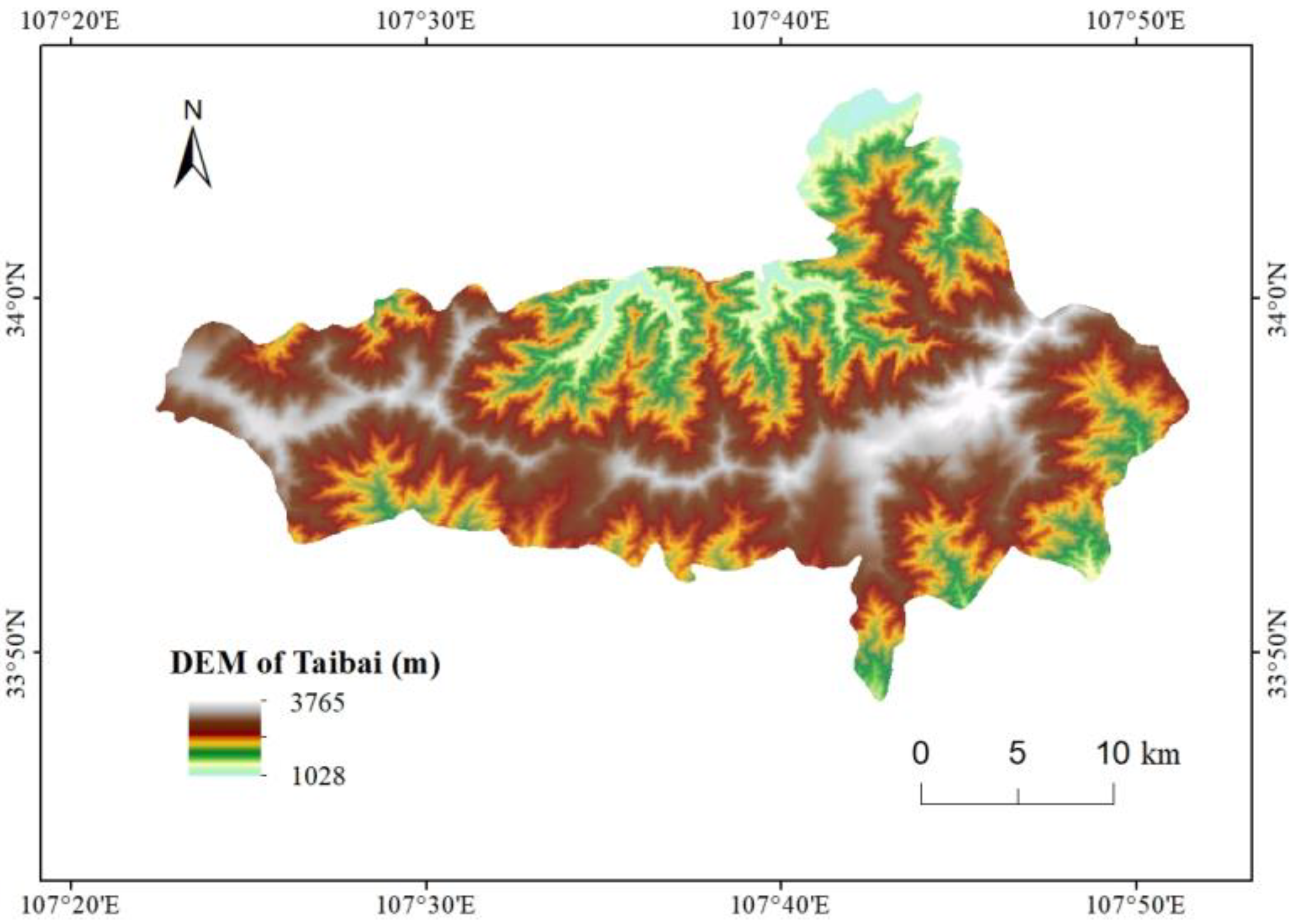
The Qinling Mountains are a well-known mountain range in central China that divides the country’s numerous natural elements into north and south [24,25]. The Taibai Mountain, the major peak of the Qinling Mountains, rises to a height of 3771 m above sea level and spans three counties: Meixian, Taibai, and Zhouzhi (107°17′ E, 107°56′ E, 33°47′ N, 34°12′ N) (Figure 1). Its average elevation is around 2050 m above sea level. Its unusual geographic position makes it an ecological transition zone and a sensitive area for climate change. It has an inland monsoon climate with low temperatures and substantial rain all year round, an average annual precipitation of 500–1100 mm, and an annual average temperature of 5.9–7.5 °C [26,27].
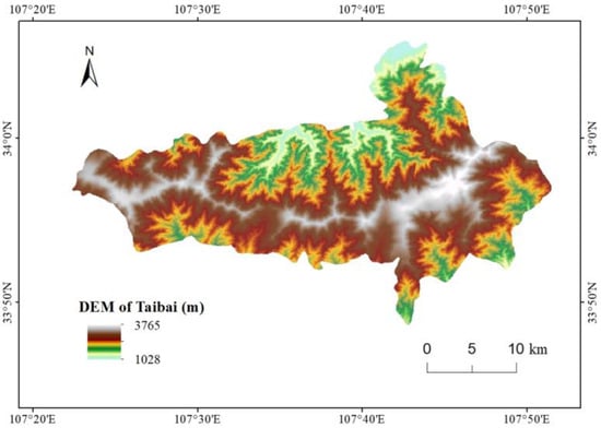
Figure 1.
Location and elevation distribution of Taibai Mountain.
The enormous height difference of the Taibai Mountain creates distinct vertical climatic, soil, and biological population zones. It is also home to national-level protected species like the giant panda (Ailuropoda melanoleuca), golden snub-nosed monkey (Rhinopithecus), antelope (Pantholops hodgsoni), and red bean fir (Taxus wallichiana), among others, making it a treasure trove of biological diversity [28]. The south slope of Taibai Mountain is steeper, less impacted by human activity, and still has a healthy amount of natural vegetation cover and vertical differentiation [29,30].
2.2. Materials
The data used in this study includes three kinds of image data and some field sampling data. (1) The NASA MODIS data product with a geographic resolution of 250 m and a temporal resolution of 16 d is used to create the NDVI data. The maximum value method (MVC) was used to create monthly NDVI, and the average value method was utilized to combine summer (June–August) and autumn (September–November) NDVI in order to remove outliers brought on by cloud coverage, (2) French SPOT5 satellite data were utilized to create the high-resolution remote sensing image, which was then combined with panchromatic and multispectral bands using the HIS variation fusion method to produce an image with a spatial resolution of 2.5 m and multispectral data, (3) the DEM has a spatial resolution of 25 m by 25 m and was produced by the First Institute of Geographic Information Cartography, Ministry of Natural Resources, China. After geographic registration, the DEM is resampled to 250 m and then analyzed with MODIS NDVI data for spatial superposition, and (4) by using a combination of manual vegetation type interpretation and handheld GPS location (whose accuracy is 3 m), the vegetation zone vertical sample data were gathered in June 2015 and June 2016.
2.3. Methods
2.3.1. Flowchart
The scatter plot of NDSA versus DEM is first created in accordance with the NDVI variation rules for various vegetation types in summer and autumn. Then, using information from the data query and the results of the field research, the structure of the NDVI-DEM scatter plot is analyzed, and the vegetation types corresponding to each region of the scatter plot are qualitatively assessed. Finally, using a binomial curve and half-peak width calculation method, the vertical zone of vegetation on Taibai Mountain was quantitatively divided. Figure 2 displays the technology roadmap.
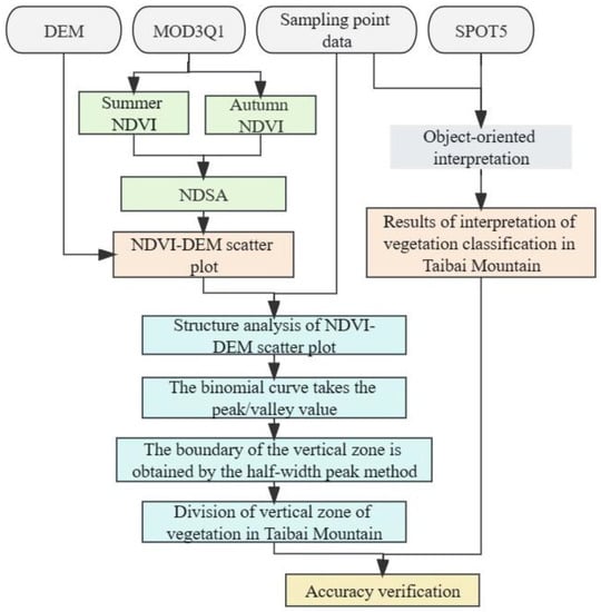
Figure 2.
Map showing the flowchart of this study.
2.3.2. Construction of a DEM-NDVI Scatter Plot
By superimposing the DEM with the NDVI, the NDVI and DEM values for each image element were calculated. The NDVI values for each elevation are acquired in 10 m steps using the sliding average approach in order to remove random fluctuations from the scatter plot. Next, the DEM-NDVI scatter plot is created using the NDVI as the vertical coordinate and the DEM as the horizontal coordinate.
2.3.3. Half-Peak Width Calculation Method
Peak width at half height (PWH; the formula refers to this as WPWH) is the width of the peak halfway above the peak, or the distance between the peak’s midpoint, a line perpendicular to its base, and its two points of intersection with its sides. The half-peak width is equal to 2.354 times the standard deviation [31]. Heat indicators for various plant zones are frequently calculated using the PWH. The following equation is employed in this study to quantify the elevation range of each vegetation vertical zone in the DEM-NDVI scatter diagram.
where X is the peak/trough value in the scatterplot structure and S is the standard deviation.
2.3.4. SPOT Image Interpretation
Vegetation types were image-interpreted using the eCognition9.0 software on the Taibai Mountain, which combined an object-oriented technique and a decision tree. The method of creating a decision tree primarily takes feature factors like color, NDVI, and elevation into account. Firstly, the spectral information was used to distinguish vegetation from non-vegetation areas (water bodies, bare rocks), then the vegetation was divided into green and yellow vegetation according to NDVI values, and then the green and yellow vegetation were classified into oak forest (Quercus acutissima), fir forest (Abies fabri), birch forest (Betula albosinensis), redwood forest (Larix chinensis), and meadows. The confusion matrix accuracy test indicated that the interpretation was 92% accurate.
3. Results
3.1. Seasonal Characteristics of the DEM-NDVI Scatter Plot
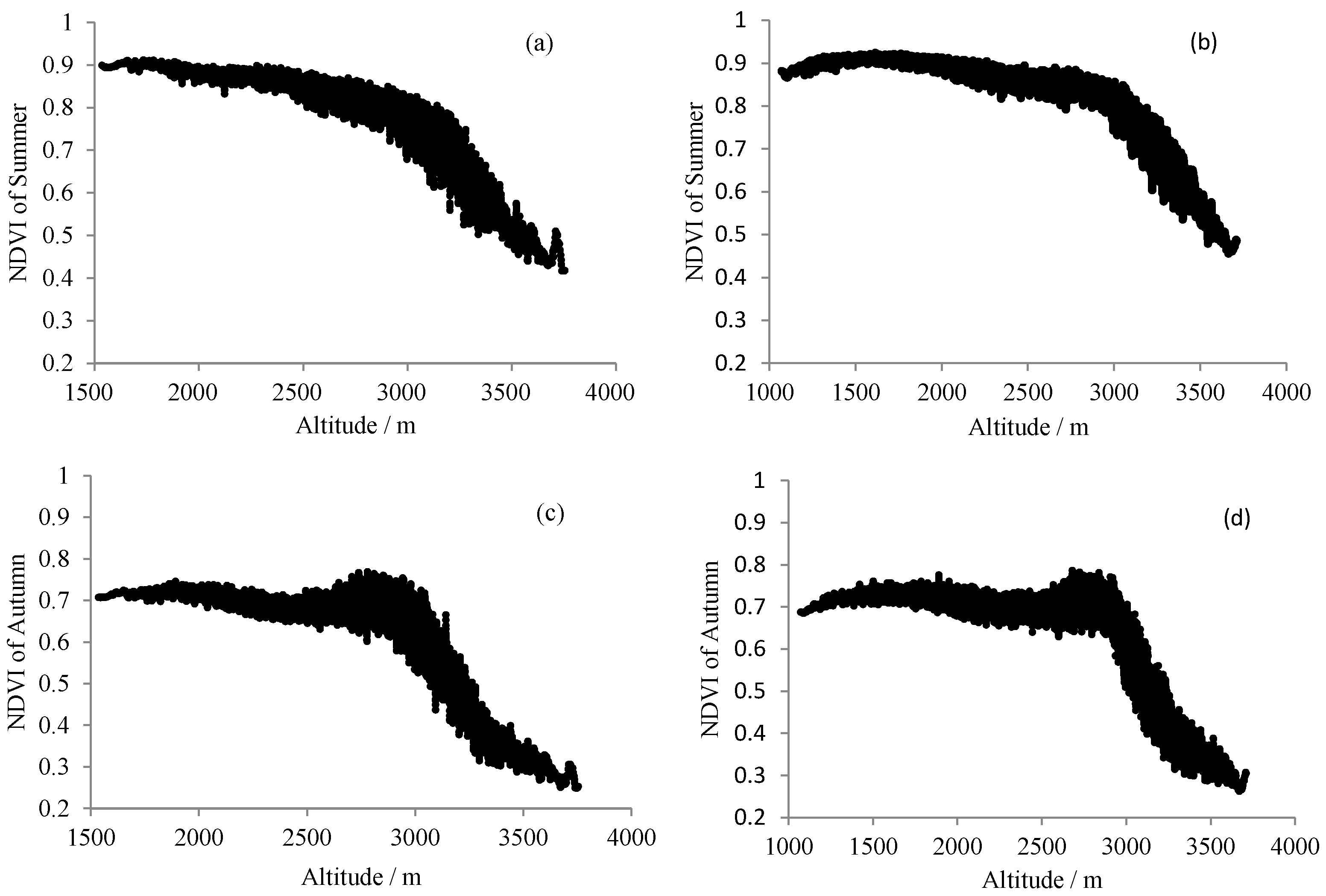
Figure 3a,b depicts the scatter plot created by the NDVI and DEM on the southern and northern slopes of Taibai Mountain in the summer, and Figure 3c,d depicts the scatter plot created by the NDVI and DEM on the southern and northern slopes of Taibai Mountain in the autumn. Figure 3 illustrates how well the vegetation of the Taibai Mountain grows in the summer. The NDVI is essentially greater than 0.8 below 2600 m, maintains 0.6 to 0.8 between 2600 and 3200 m, and drops to 0.4 at the summit’s high elevations. In the autumn, NDVI stays about 0.7 below 2600 m, reaches a small high between 2600 and 3000 m when it hits 0.75, and then rapidly decreases to 0.2–0.3.
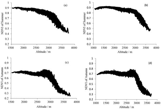
Figure 3.
Scatter plot of NDVI versus DEM on the south slope of the Taibai Mountain in summer (a); scatter plot of NDVI versus DEM on the north slope of the Taibai Mountain in summer (b); scatter plot of NDVI versus DEM on the south slope of the Taibai Mountain in summer–autumn (c); scatter plot of NDVI versus DEM on the north slope of the Taibai Mountain in summer–autumn (d).
According to the aforementioned, even though the DEM-NDVI scatter plots in summer and autumn partially reflect the vertical differentiation of the vegetation, it is still impossible to quantitatively delineate the vertical zones because, in summer, deciduous forests and evergreen forests have similar NDVI values and cannot be separated from one another, whereas, in autumn, deciduous forests and meadows have similar NDVI values and cannot be separated from one another. Therefore, the NDVI in summer or autumn alone cannot quantify the vertical zones of vegetation on Taibai Mountain. However, the NDVI difference between evergreen and deciduous forests in summer and autumn can be used to quantify the vertical zones because it is obvious.
3.2. Determination of the Vegetation’s Vertical Zone Structure Using an DEM-NDVI Scatter Plot
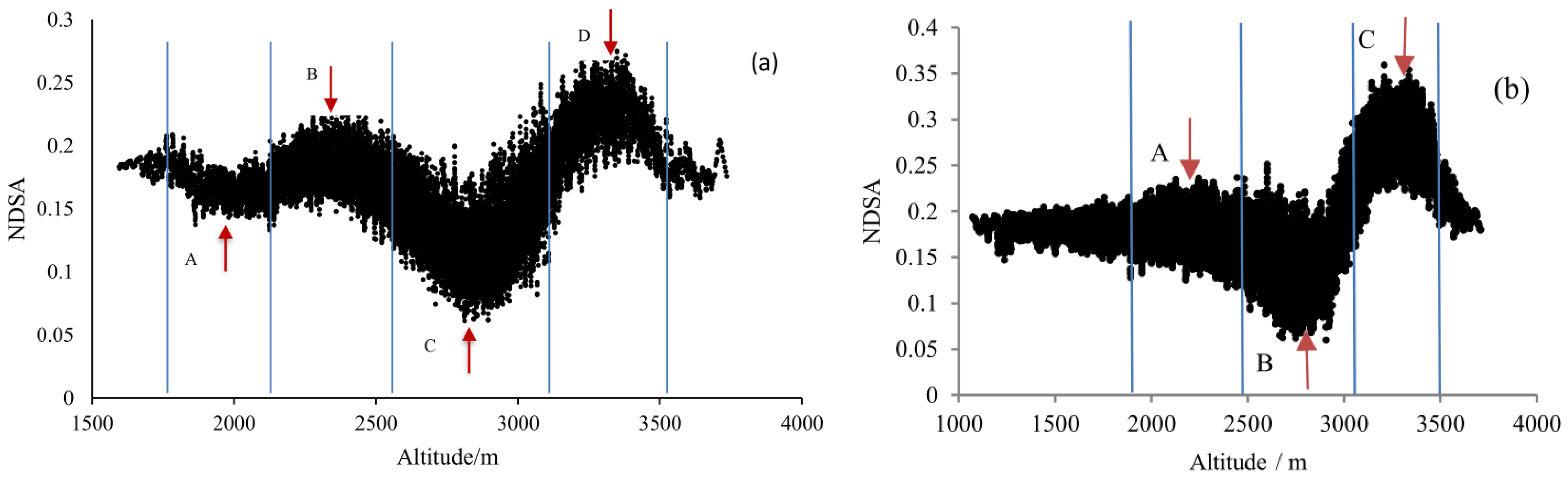
On the southern slopes and southern slopes of the Taibai Mountain Reserve, the scatter plot of NDSA versus altitude is presented in Figure 4, which depicts the zonal fluctuation of the NDVI difference with elevation in various vegetation vertical zones. The scatter plot in Figure 4 shows obvious peaks and obvious valleys, each of which represents the concentrated distribution area of a typical vegetation community. The peaks and valleys are surrounded by an interlacing zone between the typical vegetation community and other communities. The general structure of the vertical zones of vegetation on the southern slopes of Taibai Mountain can be deduced from Figure 4 using the sampling point data from the field study in June 2015 and June 2016, along with the prior knowledge on the vertical zones of Taibai Mountain [17,20,28].
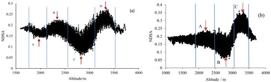
Figure 4.
Scatter plot of NDSA versus DEM on the south slope of Taibai Mountain (a); scatter plot of NDSA versus DEM on the north slope of Taibai Mountain (b).
According to Figure 4a, the overall structure of the NDSA scatter map on the south slope of Taibai Mountain can be divided into six sections. The cork oak (Quercus variabilis) and sharp-toothed oak (Quercus aliena) make up the majority of the deciduous forest in Section 1. Because the oak forest grows rapidly in the summer and begins to lose its leaves in the autumn, there is a significant difference in NDVI between summer and autumn. Between summer and autumn, there was a difference in NDVI of roughly 0.20. In Section 2, a mixed coniferous and broad forest dominated by Huashan pine (Pinus armandii), oil pine (Pinus tabuliformis), and sharp-toothed oak (Quercus serrata), the NDSA was about 0.15. This section showed a downward trend in the NDSA due to the mixing of the pine vegetation. Section 3, a mid-mountain birch forest, saw a rise in the NDSA that reached 0.23. Since birch is a deciduous tree species, there was a greater change in NDVI between summer and autumn, creating a modest wave peak in this region. Section 4 is an evergreen coniferous forest zone with fir as its dominant species. The NDSA in this section is only 0.05, the lowest value in the entire scatterplot and clearly defining a trough. In Section 5, the NDVI difference grew significantly between summer and autumn, peaking at 0.27. The redwood dominates this area’s deciduous coniferous forest belt, which has high NDVI values in the summer and rapid NDVI value declines following leaf fall in the autumn, creating a significant NDVI differential between summer and autumn. In Section 6, the NDSA declines, and it is the alpine scrub meadow zone. Alpine scrub meadows also have high summer and low autumn NDVI values, but because of their low overall coverage, even in the summer, they do not exhibit excessively high NDVI values. As a result, the NDSA is obviously smaller than it is in redwood forests.
According to Figure 4b, compared with the south slope, the NDSA scatter plot of the north slope of Taibai Mountain is flat in the band below 2000 m. The reason is that this section is subject to more human disturbance, mainly oak forest, a few pine species, and mixed with other trees, so vegetation zones cannot be clearly divided and are uniformly classified as human disturbance zones. Human disturbance zone in the first section, birch forest zone in the second section, fir forest zone in the third section, redwood forest zone in the fourth section, and alpine shrub meadow zone in the fifth section.
3.3. Determination of Vegetation Vertical Zone Boundaries Based on DEM-NDVI Scatter Plots
The binomial fitted curve and half-peak width calculation approach were used to quantify the DEM-NDVI scatterplot and determine the altitude corresponding to each vertical band. In step 1, the binomial curve for each zone of the scatter plot is plotted, and the peak and trough values (marked in red in Figure 4) and their corresponding altitudes are obtained by first-order derivation, as shown in Table 1. In step 2, the range of each zone and its corresponding altitude are calculated using the half-peak width method, as shown in Table 2.

Table 1.
The peak and valley point of the DEM-NDVI scatter plot on the south and northern slopes of Taibai Mountain.
Table 2.
The vertical division on the south slope of Taibai Mountain based on the DEM-NDVI scatter plot.
According to Table 1 and Table 2, the pure oak forest zone on the southern slope of Taibai Mountain is between 1509 and 1919 m above sea level, and at 1919 m, oil pine and huashan pine start to mix with the oak forest, with the most pine vegetation distributed at 2125 m (peak valley point A in Figure 4). Red birch gradually appears at 2115 m, and the most concentrated area is red birch at 2350 m (peak valley point B in Figure 4). Fir starts to appear at 2516 m. At 2833 m (peak and valley point C in Figure 4), the most concentrated area of fir is found, and at 3150 m, the fir gradually disappears. At 3109 m, the most concentrated area of redwood is found at 3330 m (peak and valley point D in Figure 4). At 3481 m, the redwood disappears, and above it, the alpine scrub and meadows.
Compared with the southern slope, except for the difference in the distribution of oak forest and mixed forest in the man-made disturbance zone and the south slope, the elevation of other vegetation zones was lower than that of the south slope, and the distribution width of each zone was also different from that of the south slope. The birch forest zone began to appear at 2200 m, 85 m lower than that of the south slope, and the distribution width was 20 m larger than that of the south slope. The fir forest zone began to appear at 2562 m, and the concentrated distribution area was 2714 m, 119 m lower and 132 m smaller than the south slope. Sequoia forest belt began to appear at 2987 m; the concentrated distribution area was 3250 m, 80 m lower than the south slope; and the distribution width was 84 m larger than the south slope.
3.4. Validation of the Accuracy of the DEM-NDVI Scatter Plot Vegetation Zoning
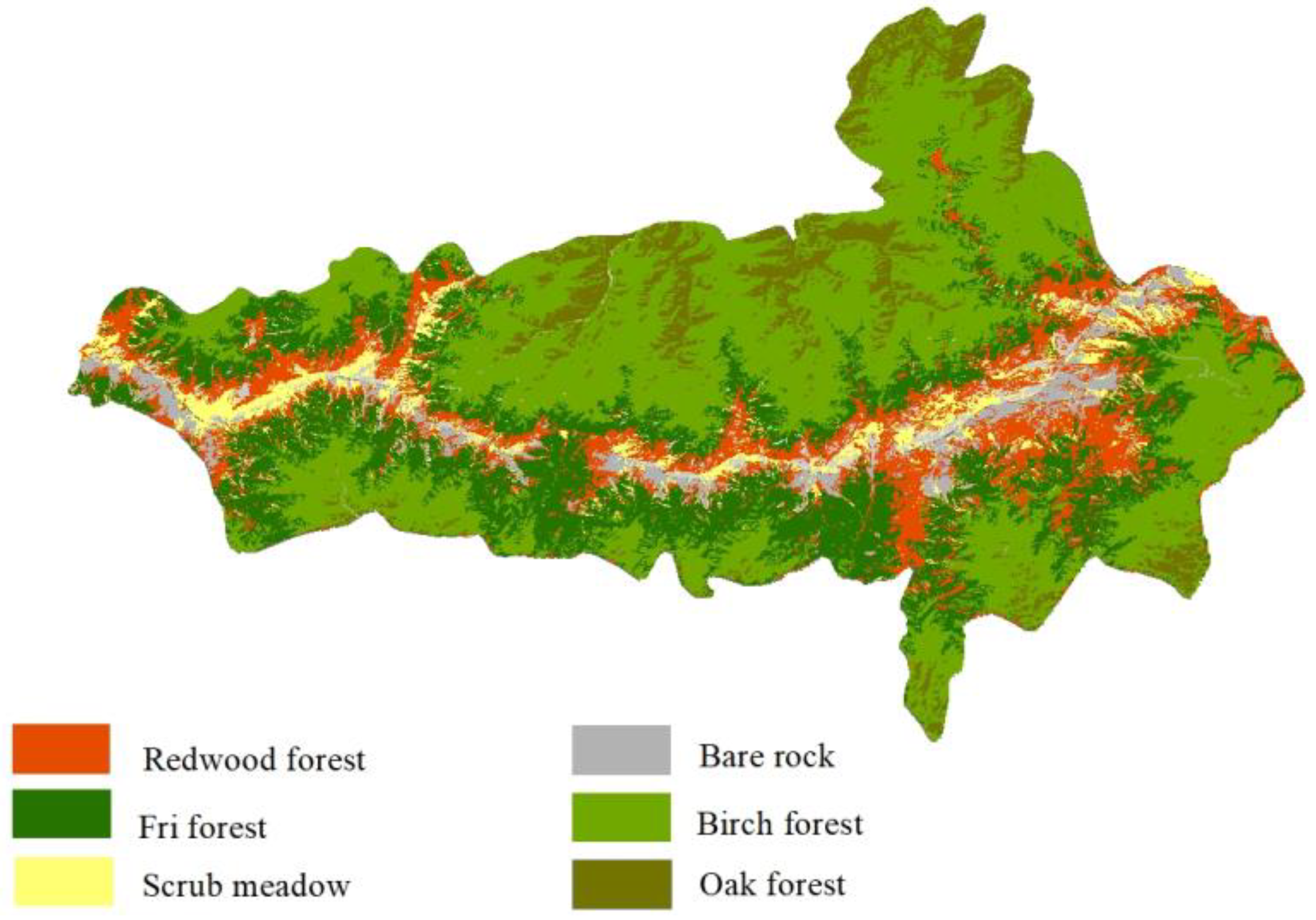
The results of the interpretation of high-resolution remote sensing pictures were compared with the vertical zone of vegetation outlined by the DEM-NDVI scatter plot in order to confirm its accuracy. The vegetation types of Taibai Mountain were deciphered using the 2.5 m resolution SPOT image, and the outcomes are depicted in Figure 5. The vertical zones of the Taibai Mountain Reserve based on remote sensing interpretation were obtained (Table 3) by superimposing the findings of remote sensing image interpretation with the DEM. The upper and lower boundaries of each vegetation zone were taken as 95% confidence intervals, with the exception of the research area boundary and the summit of the mountain, in order to exclude the elevation anomalies induced by specific picture features in the interpretation.

Figure 5.
Interpretation classification results based on a spot image of the south slope of Taibai Mountain.
Table 3.
Vertical belt distribution of Taibai Mountain based on a spot image interpretation.
It can be seen from Table 3 that the elevations of the vertical zones of vegetation interpreted by remote sensing images are as follows: cork forest is mainly distributed at a height of 2000 m, birch forest at 2500 m, fir at 2800 m, sequoia at 3200 m, and scrub meadow at 3300 m.
When Table 2 and Table 3 are compared, it can be seen that the vertical zones determined using DEM-NDVI and those acquired via remote sensing interpretation have both consistency and some differences. The differences between the two are reflected in the following: first, based on the DEM-NDVI scatter plot, it is obvious that there is a pine-oak mixed forest zone on the south slope from 1900 to 2300 m, while the vertical zone pattern interpreted by remote sensing cannot recognize this feature, which is due to the fact that the spectral features of the image can reflect well for pure forests but weakly for mixed forests. Secondly, the elevation ranges of the vertical zones based on remote sensing interpretation were significantly larger than those obtained from the DEM-NDVI scatter plot, indicating that remote sensing interpretation can capture some special vegetation groups generated by topography and ecological environment differences, while DEM-NDVI mainly reflects the average distribution of vegetation groups.
4. Discussion
4.1. Selection of Basic Materials and Methods
- (1)
- Since the classification of vertical vegetation zones by DEM-NDVI scatterplot is fast and accurate, some scholars have used this method to divide vegetation zones. However, due to the problem of mixed pixels, most studies construct DEM-NDVI scatterplots and extract vertical vegetation zones based on Landsat remote sensing images with 30 m spatial resolution [14,15,16]. For Taibai Mountain, the study area of this paper, the vertical zone of vegetation is very typical, and the vertical zone is basically pure forest. Therefore, the author tries to create a scatter map by using MODIS NDVI data with a 250 m resolution. The figure can also effectively reflect the segmented fluctuation of NDVI with elevation, indicating the effectiveness of low-resolution images in the DEM-NDVI scatter plot for delineating vegetation zones. The success of using 250 m resolution MODIS NDVI data to divide vertical zones can promote the extraction of vegetation zones in a wider range, reduce the amount of data processing, shorten the data processing time, and improve work efficiency;
- (2)
- The selection of the image data period should be flexible and varied according to the characteristics of the study area. Chang Chun et al. used autumn DEM-NDVI scatter plots to quantitatively divide the vegetation vertical zones of Wolongguan Gully [12]. In the process of this study, it was found that the vegetation vertical zones of the Taibai Mountain Protected Area could not be accurately delineated by single summer or autumn DEM-NDVI scatter plots. Therefore, the author believes that the use of DEM-NDVI scatter plots to divide the vertical zone of alpine vegetation should be flexibly applied according to the characteristics of the study area, and single-season data may cause the vertical zone of vegetation to be wrong or missing.
4.2. Discussion on the Vegetation Zone of Taibai Mountain
- (1)
- The majority of the elevations of the vertical belts of Taibai Mountain mentioned in the current literature are based on early field research, mostly in units of hundreds of meters [11,20,23]. According to Bai Hongying et al. in their book, the southern slope of Taibai Mountain is 1300 to 2300 m for oak forest, 2300 to 2600 m for birch forest, 2600 to 3200 m for fir forest, 3200 to 3400 m for redwood forest, and 3400 to the top of the mountain is 3700 m for alpine meadow [32]. In the paper of Zhang Junyao et al., the vertical vegetation zones on the southern slope of Taibai Mountain were: oak forest (1300–2000 m), red birch/pine mixed forest (2000–2300 m), red birch forest (2300–2650 m), Bashan fir forest (2650–3000 m), Taibai redwood forest (3000–3400 m), and subalpine shrub meadow (3400–3767 m) [11,33]. The vegetation vertical zone divided in this paper is very similar to the results of Zhang Junyao, which shows that the results of this study have a certain reliability. At the same time, the division of the vertical zone of vegetation has broken through the 100 m unit and reached the vegetation zone with a meter as the unit, which improves the division accuracy. In the context of climate change, how does the change in mountain altitudinal zone represent the change in mountain ecosystem [34]. However, the migration of vegetation zones is usually slow, perhaps 100 or 200 years [35], and short-term (decades) changes are often difficult to capture. In this study, the classification accuracy of vegetation zones is raised to the meter level, and the vertical zones of vegetation can be extracted according to the DEM-NDVI scatter plots of successive years, so as to realize multi-year monitoring of the changes of the vertical zones, capture the subtle information of the changes of vegetation zones, and provide data support for more accurate research;
- (2)
- There is a mixed pine oak forest on the south slope of 1900–2300 m, but no such zone on the north slope. The deep mechanism of this phenomenon needs further study. Fang Zheng and Gao Shuzhen proposed in 1963 that the reason for this phenomenon is caused by long-term anthropogenic destruction activities [30]. However, it is still worth exploring whether the development of forests in Taibai Mountain after decades of human activities is still the main reason for this phenomenon;
- (3)
- There are some differences in the division of birch forest in Taibai Mountain. Some studies believe that the vertical distribution area of birch forest should be turned into coniferous forest zone [36,37], and some people divide 2000–2650 into pine and birch forest zone [38], and some people think that birch forest, as the transition zone between warm temperate deciduous broad-leaved forest and cold temperate coniferous forest, is relatively stable in the middle of the Qinling Mountains, and it is more appropriate to divide it into Chinese forest zone [39,40]. According to the results of this study, the NDVI difference of birch forest in summer and autumn has obvious fluctuation valley points with adjacent vegetation, especially on the southern slope of Taibai Mountain. Therefore, this paper also supports the view that birch forest can be classified as a single birch forest belt from a certain angle.
4.3. Limitations and Prospects
- (1)
- The method of half-peak width calculation is often used to divide the temperature zone in physical geography [31,41]. The application of this method in this paper is a preliminary attempt to quantitatively divide the scatter-plot segment. Comparing with the results of remote sensing interpretation, it is found that the partition results are satisfactory, but they are still worth further demonstrating by other methods;
- (2)
- The binomial curve derivation method adopted in the quantitative division of DEM-NDVI scatter plot structure in this study is essentially a statistical method, and statistical methods have high requirements for data integrity and accuracy [42]. Improper selection of methods in the process of data analysis will seriously affect the scientificity of the standard. Therefore, in the process of using DEM and NDVI to divide vegetation vertical zones, some new methods, such as the cloud model [43,44,45], can be tried to better deal with the ambiguity and randomness in qualitative concepts.
5. Conclusions
In this paper, the vegetation vertical zones of Taibai Mountain were quantitatively divided according to the law of NDVI difference changing with altitude, combined with field investigation and data query, and the reliability of vertical zone division was demonstrated by field investigation of sample points and interpretation results of high-resolution remote sensing images. The main conclusions are as follows:
- (1)
- By analyzing the structure of the DEM-NDVI scatterplot in summer, autumn, and the difference between summer and autumn, the scatterplot of the difference between summer and autumn can well depict the distribution pattern of vegetation vertical zones in Taibai Mountain, and the southern slope can be divided into six vertical zones. They were the oak forest zone, pine oak mixed forest zone, birch forest zone, fir forest zone, Taibai redwood forest zone, and alpine shrub meadow zone. The southern slope can be divided into five vertical zones, namely, the human disturbance zone, the birch forest zone, the fir forest zone, the redwood forest zone, and the alpine scrub meadow zone;
- (2)
- Quantitative calculations showed that the vertical zones of vegetation on the north and south slopes of Taibai Mountain were different in height and width, as follows: from the bottom of the mountain to 2300 m, the southern slope included two vertical zones of oak forest and pine oak mixed forest, while the northern slope was a man-made disturbance zone; above 2300 m, the vertical zones of the north and south slopes have a similar distribution pattern; from bottom to top, there are birch forests, fir forests, sequoia forests, and alpine scrub meadows, respectively. The distribution height of each zone on the south slope is 80–120 m higher than that on the north slope, and the distribution width of the fir forest zone on the south slope is larger than that on the north slope, while the birch forest zone and sequoia zone on the north slope are larger than that on the south slope;
- (3)
- Compared with the results of the interpretation of vegetation classification by remote sensing images, the distribution trend of vertical zones of vegetation is roughly the same, but the DEM-NDVI scatter map can reflect the average distribution of vegetation populations and can more completely express the characteristics of vertical zones of vegetation as they change with altitude.
Author Contributions
Conceptualization, T.Z. and H.B.; methodology, T.Z. and H.H.; software, P.L.; investigation, Z.T.; resources, T.Z. and Z.T.; data curation, H.H. and P.L.; writing—original draft preparation, T.Z.; writing—review and editing, H.B. and P.W.; project administration, H.B.; research group leader, H.B. All authors have read and agreed to the published version of the manuscript.
Funding
This research was supported by a national forestry public welfare industry research project in China, grant no. 201304309; a natural science foundation of Shaanxi province, China, grant no. 2022JQ-211; a scientific research project of Shaanxi Provincial Education Department, China, grant no. 21JK0306.
Data Availability Statement
Not applicable.
Conflicts of Interest
The authors declare no conflict of interest.
References
- Liu, J.F.; Ma, S.; Li, S. Changes in vegetation NDVI from 1982 to 2016 and its responses to climate change in the black-soil area of Northeast China. Acta Ecol. Sin. 2018, 38, 7647–7657. [Google Scholar]
- Hamilton, A.C.; Perrott, R.A. A study of altitudinal zonation in the montane forest belt of Mt. Elgon, Kenya/Uganda. Vegetatio 1981, 45, 107–125. [Google Scholar] [CrossRef]
- Zhang, B.P.; Yao, Y.H. Implications of mass elevation effect for the altitudinal patterns of global ecology. J. Geogr. Sci. 2016, 26, 871–877. [Google Scholar] [CrossRef]
- Wang, Q.; Shi, M.Q.; Guo, Y.L.; Zhang, Y. The vertical differentiation of the mountain settlement niche in the upper reaches of Minjiang River. Acta Geogr. Sin. 2013, 68, 1559–1567. [Google Scholar]
- Ma, M.Z.; Shen, G.Z.; Xiong, G.M.; Zhao, C.; Xu, W.; Zhou, Y.; Xie, Z. Characteristic and representativeness of the vertical vegetation zonation along the altitudinal gradient in Shennongjia Natural Heritage. Chin. J. Plant Ecol. 2017, 41, 1127–1139. [Google Scholar]
- Li, C.G.; Tan, B.Z. Studies on the methods of mangrove inventory based on RS, GPS and GIS. J. Nat. Resour. 2003, 18, 215–221. [Google Scholar]
- Zhang, Q.Y.; Zhsng, Y.C.; Luo, P.; Wang, Q.; Wu, N. Ecological characteristics of cypress population in yang-slope forest line of Baima Mountain. Chin. J. Plant Ecol. 2007, 31, 857–864. [Google Scholar]
- Mihai, B.; Savulescu, I.; Sandric, I. Change detection analysis (1986–2002) of vegetation cover in Romania. Mt. Res. Dev. 2007, 27, 250–258. [Google Scholar] [CrossRef]
- Sitko, I.; Troll, M. Timberline changes in relation to summer farming in the western chornohora (Ukrainian carpathians). Mt. Res. Dev. 2008, 28, 263–271. [Google Scholar] [CrossRef]
- Li, W.T. Forest Vegetation Classification Using High Resolution Remote Sensing Image. Master’s Thesis, Beijing Forestry University, Beijing, China, 2016. [Google Scholar]
- Zhang, J.Y.; Yao, Y.H.; Suonan, D.; Gao, L.; Wang, J.; Zhang, X. Mapping of mountain vegetation in Taibai Mountain based on mountain altitudinal belts with remote sensing. J. Geo-Inf. Sci. 2019, 21, 1284–1294. [Google Scholar]
- Danzeglocke, J.; Oluic, M. Remote Sensing of Upper Timberline Elevation in the Alps on Different Scales. In New Strategies for European Remote Sensing; Millpress: Rotterdam, The Netherlands, 2005. [Google Scholar]
- Danzeglocke, J.; Menz, G. Analysis of upper timberline elevation in the European Alps using MODIS data. In Proceedings of the 2004 IEEE International Geoscience and Remote Sensing Symposium (IGARSS 2004), Anchorage, AK, USA, 20–24 September 2004; IEEE: New York, NY, USA, 2004; pp. 2373–2376. [Google Scholar]
- Chang, C.; Wang, X.Y.; Yang, R.X.; Liu, C.; Luo, L.; Zhen, J.; Xiang, B.; Song, J.; Liao, Y. A quantitative characterization method for alpine vegetation zone based on DEM and NDVI. Geogr. Res. 2015, 34, 2113–2123. [Google Scholar]
- Ji, X.Y.; Luo, L.; Wang, X.Y.; Li, L.; Wan, H. Identification and change analysis of mountain altitudinal zone in Tianshan bogda natural heritage site based on “DEM-NDVI-land cover classification”. J. Geo-Inf. Sci. 2018, 20, 1350–1360. [Google Scholar]
- Liao, Y. Fine Observation and Quantitative Characterization of Subalpine Vegetation Vertical Zone in Wang Lang Nature Reserve. Master’s Thesis, University of Chinese Academy of Sciences, Beijing, China, 2016. [Google Scholar]
- Yue, M. The vertical band spectrum of plants in Qinling Mountains is complete and complex. Humankind 2015, 2, 76–81. [Google Scholar]
- Yue, M.; Xu, Y.B. Qinling mountains of plants. Humankind 2014, 2, 14–25. [Google Scholar]
- Shang, S.H.; Xing, H.H. Comparison of vertical distribution of vegetation on the north and south slopes of Qinling Mountains. Agric. Jilin 2016, 1, 114–115. [Google Scholar]
- Li, H.N. Studies on the Species Diversity and Vertical Distribution Pattern on Northern Slopes of Mt. Taibai. Master’s Thesis, Shaanxi Normal University, Xi’an, China, 2007. [Google Scholar]
- Lei, M.; Chen, T.B.; Feng, L.X.; Chang, Q.R.; Yan, X. Soil formation factors and comparison among different altitudinal zonations of the soils on northern slope of the Taibai Mountains. Geogr. Res. 2001, 20, 583–592. [Google Scholar]
- Zhang, B.P.; Yao, Y.H.; Xiao, F.; Zhou, W.; Zhu, L.; Zhang, J.; Zhao, F.; Bai, H.; Wang, J.; Yu, F.; et al. The finding and significance of the super altitudinali belt of montante deciduous broad-leaved forests in central Qingling Mountains. Acta Geogr. Sin. 2022, 77, 2236–2248. [Google Scholar]
- Miehe, S.; Miehe, G. Vegetation patterns as indicators of climatic humidity in the Western Karakorum//Stellrecht I. In Karakorum-Hindukush-Himalaya: Dynamics of Change, Part I; Rüdiger Koppe Verlag: Köln, Germany, 1998; pp. 101–126. [Google Scholar]
- Kang, M.Y.; Zhu, Y. Discussion and analysis on the geo-ecological boundary in Qinling Range. Acta Ecol. Sin. 2007, 27, 2774–2784. [Google Scholar]
- Bai, H.Y.; Ma, X.P.; Gao, X.; Huo, Q. Variations in January temperature and 0℃ isothermal curve in Qinling Mountains based on DEM. Acta Geogr. Sin. 2012, 67, 1443–1450. [Google Scholar]
- Qin, J.; Bai, H.Y.; Li, S.H.; Wang, J.; Gan, Z.T.; Huang, A. Differences in growth response of Larix chinensis to climate change at the upper timberline of southern and northern slopes of Mt. Taibai in central Qinling Mountains, China. Acta Ecol. Sin. 2016, 36, 5333–5342. [Google Scholar]
- Zhang, S.H.; Bai, H.Y.; Gao, X.; He, Y.N.; Ren, Y. Spatial-temporal changes of vegetation index and its responses to regional temperature in Taibai Mountain. J. Nat. Resour. 2011, 26, 1377–1386. [Google Scholar]
- Zhai, D.P.; Bai, H.Y.; Qin, J.; Deng, C.H.; Liu, R.J.; He, H. Temporal and spatial variability of air temperature lapse rates in Mt. Taibai, Central Qinling Mountains. Acta Geogr. Sin. 2016, 71, 1587–1595. [Google Scholar]
- Li, X.D. Some understanding on the division of vertical vegetation zones on the southern slope of the western Qinling Mountains in Shaanxi Province. Shaanxi For. Sci. Technol. 1985, 3, 88–92. [Google Scholar]
- Fang, Z.; Gao, S.Z. Vertical belt spectrum of vegetation on the north and south slopes of Taibai Mountain in Qinling Mountains. Chin. J. Plant Ecol. 1963, 1, 162–163. [Google Scholar]
- Xu, W.D. Kira’s temperature indices and their application in the study of vegetation. Chin. J. Ecol. 1985, 4, 35–39. [Google Scholar]
- Bai, H.; Liu, K.; Qang, J.; Li, S.H. Vegetation Response and Adaptation in Qinling Mountains under the Background of Climate Change; Science Press: Beijing, China, 2019; p. 11. [Google Scholar]
- Fu, Z.J.; Guo, J.L. The characters of community on the vegetation of the Taibai Mountain in the Qinling. J. Baoji Teach-Er Coll. (Nat. Sci.) 1992, 1, 70–75. [Google Scholar]
- Fan, Z.M. Response analysis of gradient distribution of vegetation to climate change in Heihe River Basin. Acta Ecol. Sin. 2021, 41, 4066–4076. [Google Scholar]
- Liu, G.; Fu, B. Impacts of global climate change on forest ecosystems. J. Nat. Resour. 2001, 16, 71–78. [Google Scholar]
- Fu, Z.; Guo, J. Preliminary study of Betula Albo-Sinensis forest in Mt. Taibai. Acata Phytoecol. Sin. 1994, 18, 261–270. [Google Scholar]
- Geography Department of Shaanxi Normal University. The Annals of Geography: Ankang District of Shaanxi; Shaanxi People’s Press: Xi’an, China, 1986; pp. 364–379. [Google Scholar]
- Liu, H. The vertical zonation of mountain vegetation in China. Acta Geogr. Sin. 1981, 36, 267–279. [Google Scholar]
- Yue, M.; Dang, G.; Gu, T. Vertical zone spectrum of vegetation in Foping national nature reserve and the comparison with the adjacent areas. J. Wuhan Bot. Res. 2000, 18, 375–382. [Google Scholar]
- Zhu, Z. Stability of the Betula forest in Mt. Taibai of the Qinling Mountain range. J. Wuhan Bot. Res. 1991, 9, 169–175. [Google Scholar]
- Wang, M.; Zheng, T.; Zheng, P. Study on the relationship between distribution and heat of introduced plants in Fujian Province. J. Jiangxi Agric. Univ. 2003, 3, 383–387. [Google Scholar]
- Saouini, H.E.; Bouzid, S.; Trankil, A.; Amharref, M.; Bernoussi, A.S. Application of statistical methods for the comparative study of the degree of pollution of wastewater collected from three olive mills in Tangier-Tetouan-Al Hoceima region (Northern Morocco). J. Ecol. Eng. 2023, 24, 320–332. [Google Scholar] [CrossRef] [PubMed]
- Wu, H.; Zhen, J.; Zhang, J. Urban rail transit operation safety evaluation based on an improved CRITIC method and cloud model. J. Rail Transp. Plan. Manag. 2020, 16, 100206. [Google Scholar] [CrossRef]
- Yao, J.; Wang, G.; Xue, B.; Wang, P.; Hao, F.; Xie, G.; Peng, Y. Assessment of lake eutrophication using a novel multidimensional similarity cloud model. J. Environ. Manag. 2019, 248, 109259. [Google Scholar] [CrossRef] [PubMed]
- Mu, H.; Han, F.; Tang, X.; Wang, Z.; Wang, Z. Comparison and analysis of timberline and treeline distribution height and influencing factors of Baima Snow Mountain and Bogda Mountain based on cloud model. Geogr. Res. 2023, 42, 1941–1956. [Google Scholar]

Disclaimer/Publisher’s Note: The statements, opinions and data contained in all publications are solely those of the individual author(s) and contributor(s) and not of MDPI and/or the editor(s). MDPI and/or the editor(s) disclaim responsibility for any injury to people or property resulting from any ideas, methods, instructions or products referred to in the content. |
© 2023 by the authors. Licensee MDPI, Basel, Switzerland. This article is an open access article distributed under the terms and conditions of the Creative Commons Attribution (CC BY) license (https://creativecommons.org/licenses/by/4.0/).