Assessment of Potential Prediction and Calibration Methods of Crown Width for Dahurian Larch (Larix gmelinii Rupr.) in Northeastern China

Abstract

Crown width (CW) is an important indicator for assessing tree health, vitality, and stability, as well as being used to predict forestry models and evaluate forest dynamics. However, acquiring CW data is laborious and time-consuming, making it crucial to establish a convenient and accurate CW prediction model for forest management. In this study, we developed three models capable of conducting calibration: generalized models (GM), quantile regression models (QR), and mixed-effects models (MIXED). The aim was to effectively improve the prediction accuracy of CW using data from Dahurian larch (Larix gmelinii Rupr.) in Northeastern China. Different sampling designs were applied, including selecting the thickest, thinnest, intermediate, and random trees, with 1 to 10 sample trees for each design. The results showed that all models achieved accurate CW predictions. MIXED displayed the most superior fitting statistics than GM and QR. In model validation, with the increase in the number of sample trees, the model prediction accuracy gradually improved and the model differences gradually reduced. MIXED produced the smallest RMSE, MAE, and MAPE across all sampling designs. The intermediate tree sampling design with the best validation statistics for the given sample size was selected as the final sampling design. Under intermediate tree sampling design, MIXED required a minimum of five sample trees, while GM and QR required at least five and six sample trees for calibration, respectively. Generally, we suggested selecting MIXED as the final CW prediction model and using the intermediate tree sampling design of five trees per plot. This study could provide ideas and support for forest managers to accurately and efficiently predict CW.

1. Introduction

The exchange and conversion of material and energy between forests and the environment primarily occur through the interaction of light, water, and gases by trees [1]. The tree crown serves as the primary site for carrying out this crucial task, collectively influencing tree growth and biogeochemical cycles through the interception of light and regulation of gas and water exchange [2]. The amount of light intercepted by a tree is closely related to the distribution of leaves and branches in the crown, which holds significant importance for forest productivity and nutrient cycling [3,4,5]. Therefore, the crown width (CW), as one of the characteristics of leaf and branch distribution in horizontal space, has important research value for understanding tree architecture and forest ecosystem dynamics [6].

CW serves as a significant variable in various forestry models, including biomass models [7,8], volume models [9,10], taper equations [11,12], and basal area increment models [13], etc. Additionally, CW influences the health and vigor of trees [14], competition [15,16], and forest mortality rates [13], etc. Nevertheless, traditional manual methods of CW measurement demand substantial time and effort, which are constrained by terrain-vegetation occlusion, human perspective, and steel measuring tape deformations. Better methods of obtaining CW have also emerged with technological advances, such as LiDAR that can scan the morphology of trees throughout an entire plot [17] or remote sensing techniques that can identify tree crowns through algorithms [18,19]. However, these technologies require a high level of expertise and expensive software and hardware support to achieve accurate CW measurements. Therefore, the development of CW models using easily measurable variables for estimating CW remains a common and cost-effective choice.

Researchers had already developed numerous CW models, which served as important references for developing CW models [20,21,22,23]. But carelessly using these models may lead to substantial deviations in predictions due to the inherent variations in different tree species and established environments [24]. Therefore, it is necessary to build a model that can adapt to the distribution and changes in CW data over a broad region. It is advantageous to develop generalized CW models (GM) containing variables that reflect the attributes of the study trees and the environment in the research area, such as tree size, stand characteristics, and site characteristics to enhance predictive accuracy [25,26].

In addition to adding variables, the predictive accuracy of the CW model can be improved by using more advanced methods. Mixed-effects models (MIXED) with unique advantages usually achieve the highest predictive accuracy and are widely used [1,20,21]. On the one hand, MIXED can effectively analyze hierarchical nested data with spatial or temporal dependencies, making it less affected by heteroscedasticity and autocorrelation problems [27,28]. On the other hand, MIXED uses the empirical best linear unbiased prediction theory (EBLUP) and prior information from new stands (i.e., collecting several sample trees) to calibrate the random effects of individual stands for more accurate CW predictions [29].

Furthermore, calibration techniques applying GM and quantile regression (QR) have become prevalent in recent years to improve model prediction accuracy [30,31]. GM using the ordinary least squares method (OLS) [26] to estimate the model parameters is widely employed in modeling, and therefore research on calibrating GM has a generalizable value. However, research on GM calibration, aside from studies conducted in recent years, is limited to studies involving Hanus et al. [32] and Temesgen et al. [33]. QR is a flexible statistical method that offers several advantages, including estimates of the conditional quantile of the dependent variable distribution, not requiring further assumptions about the distribution of the error term, stronger robustness and insensitivity to outliers, and the fitted model not needing to satisfy equal variances [34,35]. Consequently, QR has been widely applied in forestry studies in recent years [30,31,36,37,38,39], and the method of combining multiple QR curves for calibration has shown promising results [30,31,38,39].

Different sampling strategies can change the prior information obtained, which may affect the accuracy of the predictions after calibration [40]. Therefore, the design and selection of sampling strategies need to strike a balance to ensure sufficiently high prediction accuracy while keeping the time and effort expended by surveyors within a reasonable range [29]. Currently, research on comparing sampling strategies for model calibration generally focuses on studying MIXED or QR separately, with relatively few comparisons between the sampling strategies of MIXED and QR [30,41]. And there is a lack of research comparing the three calibrations of models, namely MIXED, QR, and GM, in the context of CW models. Therefore, investigating the differences in results obtained from different sampling strategies for these three models during calibration would be highly meaningful.

Dahurian larch, a highly adaptable tree species to harsh climatic and soil conditions, plays a crucial role in climate change in the Far East region of the Eurasian continent [42,43]. Currently, Dahurian larch has been introduced in several countries such as Sweden and Finland [44]. Moreover, Dahurian larch plantation forests are the most common and typical research objects in Northeastern China [45]. Research on the health and stability status of Dahurian larch based on indicators such as CW is receiving increasing attention; however, there are few reports on developing CW models for Dahurian larch [21]. Therefore, the object of this study is the plantation forest of Dahurian larch, which makes up for the lack of current forestry research. Our primary goal is to develop and compare high-precision CW prediction models for Dahurian larch using different modeling methods including the generalized model (GM), mixed-effects model (MIXED), quantile regression model (QR), the corresponding calibration techniques, and a variety of sampling strategies. This study is intended to provide a broad range of ideas for CW studies of other tree species and forest management planners around the globe to ensure highly accurate and cost-effective CW predictions.

2. Materials and Methods

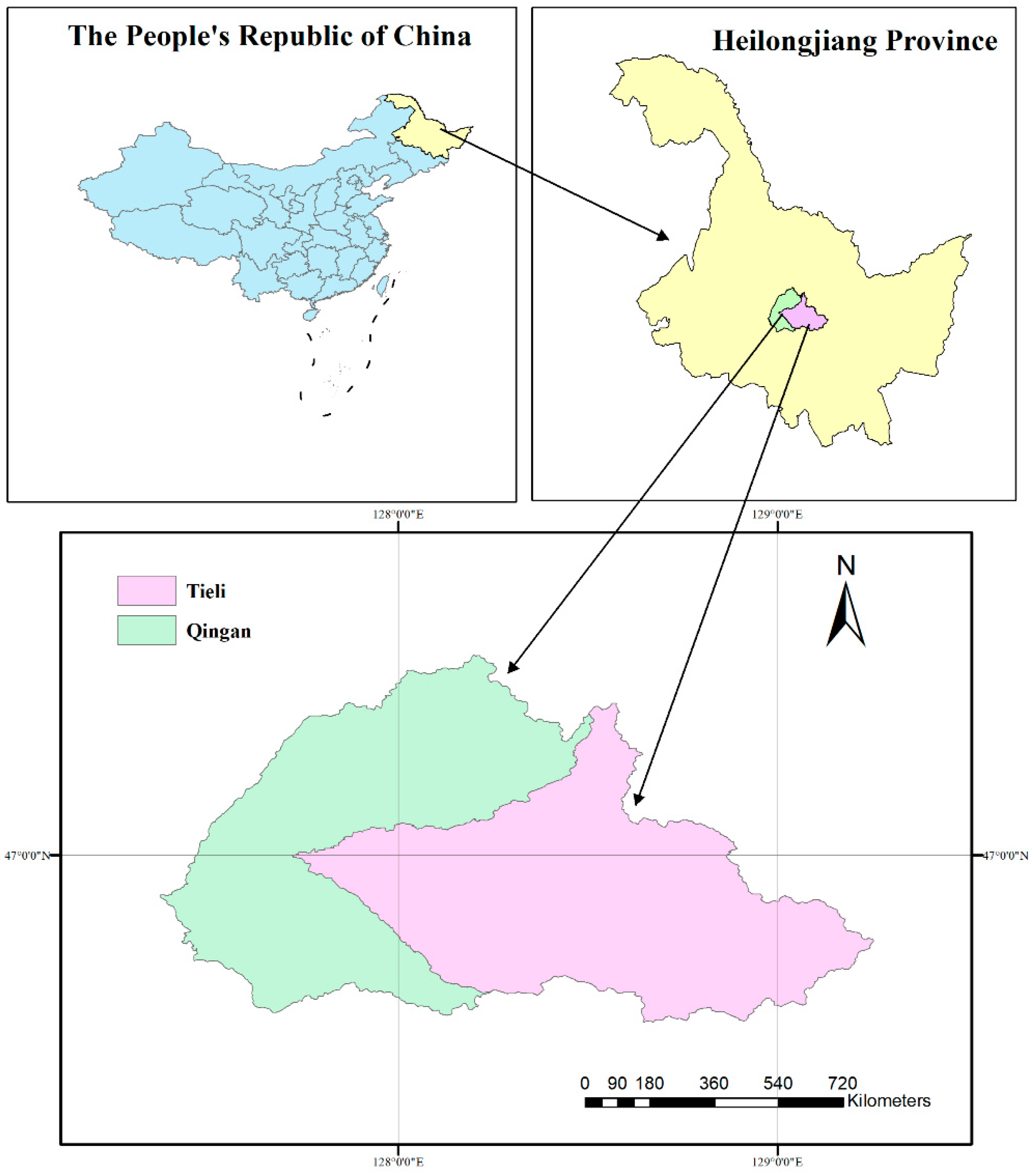
2.1. Study Area

This study focused on a sample of forests from the Weixing and Mayongshun forest farms, which are located in Tieli and Qingan, Heilongjiang Province, China (127°57′–128°12′ E, 47°02′–47°36′ N) (Figure 1). The predominant vegetation type is mixed broadleaf-conifer forest and plantations, with primary tree species including Korean pine (Pinus koraiensis Siebold and Zucc.), Dahurian larch, Scots pine (Pinus sylvestris L.), Chinese fir (Cunninghamia lanceolata (Lamb.) Hook.), ash (Fraxinus mandshurica Rupr.), elm (Ulmus pumila L. cv. Tenue), and white birch (Betula platyphylla Sukaczev). Forested lands cover an area of 0.2 million ha, with a total forest growing stock volume of 20.27 million m³, of which 11% is comprised of plantations. The average altitude is 513 m, with an annual precipitation of 831.2 mm and a mean annual temperature of 2.4 °C. The mean annual maximum and minimum temperatures are 8.8 °C and −3.4 °C, respectively. The climate in the study area is characterized by short, hot summers and predominantly long, cold, and dry winters with an extended duration of snow cover. The topography of the study site is defined by a small and flat plain in the west and low mountainous terrain in the east, which contains most of the forested areas. In China, the afforestation of Dahurian larch has been carried out for over 60 years since the founding of the country. Due to its excellent adaptability to cold climates and relatively fast growth rate, Dahurian larch has become a prominent species for reforestation and serves as a significant timber resource in China [45].

2.2. Data

In this study, we analyzed data collected in 2018 and 2019 from 62 temporary sample plots, comprising a total of 5059 Dahurian larch. Each plot had a square shape with an area of 0.09 ha. These plots were Dahurian larch plantations and exhibited no evidence of thinning, pruning, burning, severe disease, or other damage. All living trees without top damage were included in the data set for statistical analysis. Other tree species, such as ash, elm, and white birch, were present in the plots, but their numbers were too small to be included as target species in the analysis. However, they were used to calculate stand-level variables [46]. For each tree, the diameters (outside-bark 1.3 m above ground level) were measured to the nearest 0.1 cm to obtain diameter at breast height (D, cm). We retained all trees with D ≥ 5 cm and measured other variables, including total tree height (H, m) and height to crown base (HCB, m), with a precision of 0.1 m (measured using a Vertex IV ultrasonic hypsometer). We used the vertical sighting method [47] by looking up and walking to the edge of the crown in four different directions (north, east, south and west). The horizontal distance from the center of the trunk to the location (CR_n, CR_e, CR_s, and CR_w) was then measured with the help of a tape measure and a laser range finder. For the same crown radius, three or more measurers were asked to repeat the measurements and then the average value was calculated as the final value of the crown radius. CW was calculated by (CR_e + CR_s + CR_w + CR_n)/2 [1,28].

Several stand variables were counted and calculated to facilitate the development of generalized CW models. These variables included the dominant tree height (HDOM, m), dominant tree diameter (DDOM, cm), quadratic mean diameter (Dq, cm), basal area of the stand (BA, m²·ha⁻¹), basal area of trees larger than the subject tree (BAL, m²·ha⁻¹), and stem numbers (N, trees·ha⁻¹). According to the IUFRO (International Union of Forest Research Organizations), HDOM was calculated as the average height of the 100 largest trees per hectare based on the plot area [48]. Additionally, the H-to-D ratio (HDR) and relative spacing index (RSI), D-to-Dq ratio (DQMD), and Reineke’s stand density index (SDI) have all been included as important candidate predictor variables in this paper [20,49]. Due to incomplete data collection during the data gathering process, information regarding stand age for various sites was not fully obtained. Therefore, stand age was not included in the modeling process. All the above variables were easily accessible and calculated through conventional methods, making the models user-friendly and practical for application.

Table 1. Summary statistics for Dahurian larch (Larix gmelinii Rupr.) sample trees of the whole data.

Variable	Description	Min	Max	Average	SD
D (cm)	Diameter at breast height	5.0	62.0	18.1	6.2
H (m)	Total tree height	3.8	29.7	17.0	3.6
HCB (m)	Height to crown base	1.7	21.0	11.5	2.6
CW (m)	Crown width	0.15	8.30	2.97	1.00
HDOM (m)	Dominant tree height	18.36	28.54	21.16	2.18
DDOM (cm)	Dominant diameter	21.92	51.00	27.43	5.03
Dq (cm)	Quadratic mean diameter	15.12	35.87	17.66	3.70
BA (m2·ha−1)	Basal area per hectare	23.56	39.62	30.43	2.93
BAL (m2·ha−1)	Basal area of trees larger than the subject tree	0.00	38.36	18.22	8.58
N (trees·ha−1)	Stem numbers	333	1778	1324	293
HDR	H-to-D ratio	0.44	1.83	0.98	0.18
DQMD	D-to-Dq ratio	0.20	2.09	1.02	0.25
RSI	Relative spacing index	0.11	0.20	0.13	0.01
SDI	Reineke’s stand density index	514.61	874.53	697.40	63.79

provides a detailed summary of the data used in the analyses.

2.3. Generalized Model

2.3.1. Basic Model

The study utilized the commonly used nine CW-D models in the literature as candidates (

Table 2. Candidate basic models and fitting statistics.

Model	Function Form	R2	RMSE	AIC	SD
Linear	$\mathrm{CW}={\beta }_0+{\beta }_1\mathrm{D}$	0.5191	0.6933	10,647.81	0.5191
Power	$\mathrm{CW}={\beta }_0{\mathrm{D}}^{{\beta }_1}$	0.5343	0.6821	10,493.82	0.5343
Compund	$\mathrm{CW}={\beta }_0{{\beta }_1}^{\mathrm{D}}$	0.4564	0.7375	11,269.72	0.4564
Quadratic	$\mathrm{CW}={\beta }_0+{\beta }_1\mathrm{D}+{\beta }_2{\mathrm{D}}^2$	0.5512	0.6693	10,300.61	0.5512
Hossfeld I	$\mathrm{CW}={(\mathrm{D}/({\beta }_0+{\beta }_1\mathrm{D}))}^2$	0.5504	0.6704	10,315.13	0.5504
Growth	$\mathrm{CW}=exp({\beta }_0+{\beta }_1\mathrm{D})$	0.4565	0.7376	11,269.72	0.4565
Exponential	$\mathrm{CW}={\beta }_{0}exp({\beta }_1\mathrm{D})$	0.4565	0.7372	11,269.74	0.4565
Monomolecular	$\mathrm{CW}={\beta }_0(1-exp(-{\beta }_1\mathrm{D}\left)\right)$	0.5461	0.6734	10,354.43	0.5461
Logistic	$\mathrm{CW}={\beta }_0/(1+exp({\beta }_1\mathrm{D}+{\beta }_2\left)\right)$	0.5583	0.6645	10,225.33	0.5583

) [26,50,51]. The data were input into these models to obtain CW predictions. The coefficient of determination (R²), root mean square error (RMSE), and Akaike information criterion (AIC) were calculated for each model and compared to select the optimal basic model.

2.3.2. Variable Selection

Tree size, site characteristics, and stand characteristics variables were included in the optimal basic model through the two-stage approach [27,28]. In the first stage, we fitted the basic model to the data for each plot separately; however, the model for some plots could not converge. Therefore, we fitted the mixed-effects model of the basic model to obtain random-effect parameters for each plot. The location of the random-effect parameters of the best-fitting model was used as the location of the added variable. The Pearson correlation plots of the random effect parameters for each plot were then plotted against all variables. In the second stage, the basic model was expanded through reparameterization to incorporate variables that were closely correlated with the parameters.

A priori analysis showed no variance heterogeneity across the range of predicted values, and therefore no variance function was applied for GM and MIXED. The effect of a covariate on variations in CW was evaluated graphically by incrementally changing a covariate variable at equal intervals while keeping the other variables at their mean values. The GM was fitted using the “nls” function in R software version 4.2.1 (R Foundation for Statistical Computing, Vienna, Austria) [52].

2.4. Mixed-Effects Model

We incorporated plot-level random effects into GM using the nonlinear mixed-effects modeling approach. The variation in random effect parameters in mixed-effects models can partially explain the differences in covariate values between groups or represent inter-group variability that cannot be explained in some applications [28,53]. The matrix form of the expression for the nonlinear mixed-effects model (MIXED) is defined as follows:

$$\begin{array}{c}{\mathrm{CW}}_{ij}=f({\phi }_i,x_{ij})+{\epsilon }_{ij},{\phi }_i=A_i\beta +B_i{b}_i\\ {\epsilon }_{ij}~N\left(0,{\mathrm{R}}_i\right),{\mathrm{R}}_i={\sigma }^2{\mathrm{G}}_i^{0.5}{\mathsf{\Gamma }}_i{\mathrm{G}}_i^{0.5}\\ b_i~N\left(0,\mathrm{D}\right)\end{array}$$

(1)

where CW_ij is the CW of the jth sample tree in the ith sample plot, x_ij is a vector for measurements of predictor variables on plot i, φ_i is the particular parameter of plot i, ε_ij is the error term of the normal distribution within the sample plot. A_i and B_i are the design matrices, β is a p × 1 dimensional vector of fixed parameters, b_i is a q × 1 dimensional vector for plot-level random effect parameters and is assumed to have a multivariate normal distribution with a zero mean and respective variance–covariance matrix D. R_i is the variance–covariance matrix within the plot where σ² is the residual variance common to all plots, Γ_i is a matrix accounting for within-plot autocorrelations of the residuals, and G_i is a diagonal matrix accounting for the variance in within-plot heteroscedasticity. The “nlme” function of R software version 4.2.1 and the “nlme” package were used to estimate the random effect parameters [52].

2.5. Quantile Regression

Quantile regression offers a more complete picture of the relationship between variables by estimating multiple rates of change from the minimum to the maximum response. The parameters of quantile regression (QR) are obtained by minimizing the asymmetric loss function of the absolute values of the residuals as follows [54]:

$$\mathrm{S}=\left[{\displaystyle \sum _{y_{ij}\ge {\widehat{y}}_{ij}^{\tau }}\tau }\left(y_{ij}-{\widehat{y}}_{ij}^{\tau }\right)+{\displaystyle \sum _{y_{ij}<{\widehat{y}}_{ij}^{\tau }}\left(1-\tau \right)}\left(y_{ij}-{\widehat{y}}_{ij}^{\tau }\right)\right]$$

(2)

where ${\widehat{y}}_{ij}^{\tau }$ is the predicted value of CW in the τth quantile model, and y_ij is the measured value of CW. A series of QRs (τ = 0.1, 0.2, 0.3, 0.4, 0.5, 0.6, 0.7, 0.8, 0.9) were constructed to fit the entire dataset, by using the “nlqr” function in the “quantreg” package of R software version 4.2.1 [52].

2.6. Predictive Ability of Different Models

2.6.1. Calibration Technique of GM

If the response variable of a subsample of n_ij trees from the ith plot is known, this prior information could improve the prediction accuracy of the response variable for the remaining trees in the same plot. The correction factor $k_i^{*}$ could be calibrated using the following formula [33]:

$$k_i^{*}={\displaystyle \sum _{j=1}^{n_{ij}}\left({\widehat{\mathrm{CW}}}_{ij}\ast {\mathrm{CW}}_{ij}\right)}/{\displaystyle \sum _{j=1}^{n_i}{\left({\widehat{\mathrm{CW}}}_{ij}\right)}^2}$$

(3)

where $\widehat{\mathrm{C}{\mathrm{W}}_{ij}}$ is the predicted CW from GM for the jth subsample tree in the ith plot. $\mathrm{C}{\mathrm{W}}_{ij}$ is the observed CW value of the jth subsample tree in the ith plot. n_ij is the number of sample trees used for calibration in the ith plot. Then, multiplying the correction factor $k_i^{*}$ with the GM gives the calibration model (GMC). The function form of GMC is as follows:

$${\mathrm{CW}}_{ij}=k_i^{\ast }\times \mathrm{GM}$$

(4)

2.6.2. Calibration Technique of MIXED

The plot-specific random effects parameter of the ith plot could be predicted by using the first-order Taylor series expansion based on the subsample of trees in the same plot [53,55]. The random effects parameter ${\widehat{b}}_i^{\left(k\right)}$ is shown as follows:

$${\widehat{b}}_i^{\left(k\right)}=\widehat{\mathrm{D}}{\mathrm{Z}}_i^{\mathrm{T}}{\left({\mathrm{Z}}_i\widehat{\mathrm{D}}{\mathrm{Z}}_i^{\mathrm{T}}+{\widehat{\mathrm{R}}}_i\right)}^{-1}\left({\mathrm{y}}_i-\mathrm{f}\left({\mathrm{x}}_i,\widehat{\mathsf{\beta }},{\widehat{b}}_i^{\left(k-1\right)}\right)+{\mathrm{Z}}_i{\widehat{b}}_i^{\left(k-1\right)}\right)$$

(5)

where $\widehat{\mathsf{\beta }}$ is a vector of fixed-effect parameters $\beta$, $\widehat{\mathrm{D}}$ is the variance–covariance matrix at the sample site level, ${\widehat{\mathrm{R}}}_i$ is the error matrix, ${\mathrm{Z}}_i$ is the partial derivative of the function f with respect to $b_i$, shaped as ${\left.\frac{\partial f(x_i,\mathsf{\beta },b_i)}{\partial b_i}\right|}_{\widehat{\beta },b_i}$, and y_i is a vector of measured values of CW.

Since both ends of Equation (5) contain random effect parameters ${\widehat{b}}_i$, we used an iterative process to solve it [56]. In this process, ${\widehat{b}}_i^{\left(k\right)}$ represents the estimated value of the random effect parameter for plot i in the k-th iteration. When the k-th iteration is completed and $|{\widehat{b}}_i^{\left(k\right)}-{\widehat{b}}_i^{\left(k-1\right)}|<1\times {10}^{-6}$ is reached, ${\widehat{b}}_i^{\left(k\right)}$ represents the final estimate of the random effect parameter. It is added to the specified fixed-effect parameters to calculate the predicted CW:

$${\widehat{\mathrm{y}}}_i=f\left(x_i,\widehat{\mathsf{\beta }},{\widehat{b}}_i^{\left(k\right)}\right)$$

(6)

2.6.3. Calibration Technique of QR

The goal of QR calibration is to improve prediction accuracy by identifying the quantile curve or the two closest quantile curves that the subsample of trees in each plot pass through [30,38,39]. The calibration formula for QR is shown as follows:

$${\widehat{\mathrm{CW}}}_{ij}=\alpha {\widehat{y}}_k\left(x_{ij}\right)+\left(1-\alpha \right){\widehat{y}}_{k+1}\left(x_{ij}\right)$$

(7)

where $\widehat{\mathrm{C}{\mathrm{W}}_{ij}}$ is the predicted CW of calibration, ${\widehat{y}}_k\left({\mathbf{x}}_{ij}\right)$ and ${\widehat{y}}_{k+1}\left({\mathbf{x}}_{ij}\right)$ are the predicted CW of the two closest curves of a group of quantile curves, and α is the interpolation ratio in the form $\mathsf{\alpha }=\frac{{\widehat{y}}_{k+1}\left({\mathrm{x}}_{ij}\right)-\mathrm{C}{\mathrm{W}}_{ij}}{{\widehat{y}}_{k+1}\left({\mathrm{x}}_{ij}\right)-{\widehat{y}}_k\left({\mathrm{x}}_{ij}\right)}$.

The calibration process was divided into two cases: measuring the CW of either a single tree or multiple trees in each plot. When measuring CW for a single tree, two quantile curves were selected to encompass CW_ij (i.e., ${\widehat{y}}_k\left({\mathbf{x}}_{ij}\right)$ ≤ $\mathrm{C}{\mathrm{W}}_{ij}$ ≤ ${\widehat{y}}_{k+1}\left({\mathbf{x}}_{ij}\right)$), and a calibrated CW curve passing through that point was obtained by interpolation using Equation (7). If the CW is higher than the maximum (qth) quantile curve, ${\widehat{y}}_k$ is defined as ${\widehat{y}}_{q-1}$, ${\widehat{y}}_{k+1}$ is defined as ${\widehat{y}}_q$. Similarly, if the CW is lower than the minimum (1st) quantile curve, ${\widehat{y}}_k$ and ${\widehat{y}}_{k+1}$ are defined as ${\widehat{y}}_1$ and ${\widehat{y}}_2$, respectively.

When measuring the CW of multiple trees, the calibration process involves finding the two quantile curves with sign changes that correspond to the mean bias error (MBE) between the observed CWs (CW_obv) and predicted CWs (CW_pre) of the sampled trees for each plot (i.e., $\mathrm{MBE}=\frac{1}{\mathrm{n}}{\sum }_{\mathrm{j}=1}^{\mathrm{n}}(\mathrm{C}{\mathrm{W}}_{obv}-\mathrm{C}{\mathrm{W}}_{pre})$ at τ = k, MBE > 0; at τ = k + 1, MBE < 0), the interpolation ratio α is minimized by computing ${\sum }_{\mathrm{j}=1}^{\mathrm{n}}(\mathrm{C}{\mathrm{W}}_{obv}-\mathrm{C}{\mathrm{W}}_{pre}{)}^2$, and $\alpha$ is substituted into Equation (7) to complete the calibration. In cases where most of the CW_obv values are lower than the CW_pre values of the minimum quantile (k = 1) curve (i.e., MBE < 0 in all quantile curves), ${\widehat{y}}_k$ and ${\widehat{y}}_{k+1}$ are defined as ${\widehat{y}}_1$ and ${\widehat{y}}_2$, respectively. Similarly, if most of the CW_obv values are larger than the CW_pre values of the maximum quantile (k = q) curve (i.e., MBE > 0 in all quantile curves), then ${\widehat{y}}_k$ is defined as ${\widehat{y}}_{q-1}$, and ${\widehat{y}}_{k+1}$ is defined as ${\widehat{y}}_q$.

Four combinations of quantile regression for calibration (QRC), containing three-quantiles (QRC3, τ = 0.1, 0.5, and 0.9), five-quantiles (QRC5, τ = 0.1, 0.3, 0.5, 0.7, and 0.9), seven-quantiles (QRC7, τ = 0.1, 0.3, 0.4, 0.5, 0.6, 0.7, and 0.9), and nine-quantiles (QRC9, τ = 0.1, 0.2, 0.3, 0.4, 0.5, 0.6, 0.7, 0.8, and 0.9) were compared. The optimal QRC was then compared with GMC and MIXED.

2.7. Sample Alternatives in Prediction

Different sampling designs and sample sizes can change the correction factor $k_i^{*}$, random effects parameters ${\widehat{b}}_i^{\left(k\right)}$, and interpolation ratio α in the above models, leading to variations in the accuracy of CW predictions. Therefore, several strategies of tree selection were compared for the models used in this study, including:

• Selecting the 1 to 10 thickest sample trees from each plot for calibration;
• Selecting the 1 to 10 sample trees that have DBH closest to the arithmetic average of all the sample trees from each plot for calibration;
• Selecting the 1 to 10 thinnest sample trees from each plot for calibration;
• Randomly selecting 1 to 10 sample trees from each plot for calibration, repeating the process 50 times, and calculating the average to reduce the extreme calibration results due to randomness.

Since the uncalibrated models were not subject to sampling, the model parameters remained unchanged. Previous research had demonstrated that selecting fewer than 10 sample trees was the most sensible option, taking into account the fluctuations in prediction accuracy and practical application [57]. The selection of sample size can be achieved by assessing the RMSE variation rates (ΔRMSE).

2.8. Model Estimation and Evaluation

All the fitting and validation statistics of the models were obtained using R software in version 4.2.1 [52]. A self-written function was used for model calibration, and the graphical results of the models were obtained using various functions from the “ggplot2” package [52]. The models were validated using leave-one-out cross-validation (LOOCV), with each plot being used as the validation data and the remaining plots as the fitting data. The fitting statistics of the models used R-squared (R²) and root-mean-square error (RMSE), while the validation statistics used RMSE, mean absolute error (MAE), and mean absolute percentage error (MAPE). The calculated evaluation statistics for fitting and validating are as follows:

$${\mathrm{R}}^2=1-\frac{{\displaystyle \sum _{i=1}^m{\displaystyle \sum _{j=1}^n{({\mathrm{CW}}_{ij}-\widehat{{\mathrm{CW}}_{ij}})}^2}}}{{\displaystyle \sum _{i=1}^m{\displaystyle \sum _{j=1}^n{({\mathrm{CW}}_{ij}-\overline{{\mathrm{CW}}_i})}^2}}}$$

(8)

$$\mathrm{RMSE}=\sqrt{\frac{1}{{\displaystyle \sum _{i=1}^{m}n}}{\displaystyle \sum _{i=1}^m{\displaystyle \sum _{j=1}^n{({\mathrm{CW}}_{ij}-\widehat{{\mathrm{CW}}_{ij}})}^2}}}$$

(9)

$$\mathrm{MAE}=\frac{{\displaystyle \sum _{i=1}^m{\displaystyle \sum _{j=1}^n|{\mathrm{CW}}_{ij}-\widehat{{\mathrm{CW}}_{ij}}|}}}{{\displaystyle \sum _{i=1}^{m}n}}$$

(10)

$$\mathrm{MAPE}=\frac{1}{{\displaystyle \sum _{i=1}^{m}n}}{\displaystyle \sum _{i=1}^m{\displaystyle \sum _{j=1}^n\left|\frac{{\mathrm{CW}}_{ij}-\widehat{{\mathrm{CW}}_{ij}}}{{\mathrm{CW}}_{ij}}\right|}}\times 100$$

(11)

$$\Delta \mathrm{RMSE}=\frac{RMS{E}_{(Sample=1)}-RMS{E}_{(Sample=i)}}{RMS{E}_{(Sample=1)}}\times 100$$

(12)

where $\mathrm{C}{\mathrm{W}}_{ij}$ is the observed value of the jth tree CW in the ith plot, $\widehat{\mathrm{C}{\mathrm{W}}_{ij}}$ is the model predicted value of $\mathrm{C}{\mathrm{W}}_{ij}$, $\overline{\mathrm{C}{\mathrm{W}}_i}$ is the average value of CW in the ith plot, m is the number of plots, and n is the number of trees per plot, ${\mathrm{RMSE}}_{(\mathit{\text{Sample}}=1)}$ is the RMSE value of sample size = 1, and ${\mathrm{RMSE}}_{\left(\mathit{\text{Sample}}=i\right)}$ is the RMSE value of sample size = i.

3. Results

3.1. Generalized Model

The forms and fitting statistics of the nine candidate base models are presented in Table 2. The parameter estimation values of all models were statistically significant (p < 0.05). The logistic model had the highest R² and the lowest RMSE and AIC values, making it the optimal choice as the basic model for predicting CW. The basic model is shown as follows:

$$\mathrm{CW}=\frac{{\beta }_0}{1+exp({\beta }_1\mathrm{D}+{\beta }_2)}$$

(13)

where CW and D are the respective crown width and the diameter at breast height of each tree; ${\beta }_0$, ${\beta }_1$ and ${\beta }_2$ are the model parameters.

The likelihood ratio tests for different random-effects parameters for the mixed-effects model form of the basic model are shown in

Table 3. Likelihood ratio tests (LRT) for basic model with different random-effects parameters.

Random Parameter	df	AIC	BIC	Log-Lik	LRT	p-Value
β0	6	8242.206	8281.380	−4115.103
β1	6	8179.481	8218.654	−4083.740
β2	6	8125.910	8165.084	−4056.955
β0, β1	8	8119.116	8171.347	−4051.558	10.7945	0.0045
β1, β2	8	8005.991	8058.222	−3994.995

. Adding the random-effects parameters to β₁ and β₂ of Equation (13) yielded the smallest AIC and BIC values, indicating that they were the optimal positions for incorporating the variables. The Pearson correlation coefficients (r) between the random-effect parameters added to β₁ and β₂ and the variables in Table 1 are depicted in Figure 2. The parameter β₁ of the basic model had a strong correlation with Dq, HDOM, and DDOM (r > 0.6). The parameter β₂ had a moderate correlation with H, N, Dq, HDOM, and DDOM (0.4 < r < 0.6). Different combinations of variables with moderate and strong correlations with parameters were added to the model for fitting. The best combination of variables added to the model was selected based on the fitting statistics RMSE and R². The GM is shown as follows:

$$\mathrm{CW}=\frac{{\beta }_0}{1+exp(({\beta }_1+{\beta }_3\mathrm{Dq})\mathrm{D}+({\beta }_2+{\beta }_4\mathrm{HDOM}))}$$

(14)

where Dq is the quadratic mean diameter of each plot; HDOM is the dominant tree height of each plot; β₃ and β₄ are the model parameters to be estimated; and other abbreviations have been defined in Equation (13).

The CW prediction curves of the GM are shown in Figure 3 for the influence of Dq and HDOM on CW. CW increased as HDOM increased and decreased as Dq increased. As the D increased, the differences in curves within the Dq became more pronounced, while those within the HDOM became less noticeable.

3.2. Mixed-Effects Model

Mixed-effects models were established according to Equation (14). There were 31 different combinations of random-effect parameters, of which 18 converged. A comparison of the optimal mixed-effects models for choosing different numbers of random-effects parameters is shown in

Table 4. Likelihood ratio tests (LRT) for MIXED with different random-effects parameters.

Random Parameter	df	AIC	BIC	Log-Lik	LRT	p-Value
None	6	9984.156	10,023.329	−4986.078
β0	8	8018.339	8070.570	−4001.170	1969.8165	<0.0001
β0, β4	10	7913.663	7978.952	−3946.831	108.6763	<0.0001
β1, β2, β3	13	7935.892	8020.768	−3954.946	16.2297	0.001

. The random-effects parameters b₀ and b₁ had the lowest AIC and BIC values and the highest log-likelihood, making them the most optimal form of MIXED:

$$\mathrm{CW}=\frac{{\beta }_0+b_0}{1+exp((({\beta }_1+{\beta }_3\mathrm{Dq})\mathrm{D}+({\beta }_2+({\beta }_4+b_1)\mathrm{HDOM})))}$$

(15)

where b₀ and b₁ are the random-effects parameters; other abbreviations have been defined in Equation (14).

3.3. Quantile Regression

The same function form in Equation (14) was used to predict the τth CW quantile as follows:

$${\mathrm{CW}}^{\tau }=\frac{{\beta }_0^{\tau }}{1+exp((({\beta }_1^{\tau }+{\beta }_3^{\tau }\mathrm{Dq})\mathrm{D}+({\beta }_2^{\tau }+{\beta }_4^{\tau }\mathrm{HDOM})))}$$

(16)

where $\mathrm{C}{\mathrm{W}}^{\tau }$ is the predicted value of the τth quantile crown width, ${\beta }_0^{\tau }$~${\beta }_4^{\tau }$ is the parameter of the τth QR of CW, and the other abbreviations have been defined in Equation (14).

Figure 4 shows the various CW simulation curves based on quantiles (τ = 0.1, 0.2, 0.3, 0.4,0.5, 0.6, 0.7, 0.8, and 0.9). The QR curves did not show a significant simulation curve crossover at the points of maximum and minimum D, which suggested that they effectively reflected the distribution of CW. In addition, the simulation curve of GM has been included in Figure 4, and its shape closely resembles that of the median curve (τ = 0.5). The two curves almost completely overlap, except for the extreme values of D. These findings indicated that the distribution of CW in this study was uniform, and the mean value of the CW was similar to the median value.

3.4. Model Fitting

The model parameters and fitting statistics are presented in

Table 5. Parameter estimates (Par) and fit statistics (Stat) calculated using the whole dataset for the GM, MIXED, and QR at nine quantiles (τ = 0.1, 0.2, 0.3, 0.4, 0.5, 0.6, 0.7, 0.8, and 0.9).

Par/Stat	GM	MIXED	QR
			τ = 0.1	τ = 0.2	τ = 0.3	τ = 0.4	τ = 0.5	τ = 0.6	τ = 0.7	τ = 0.8	τ = 0.9
β0	6.0908	5.9724	4.3750	4.7382	4.9205	5.2849	5.4180	5.7644	6.2322	7.1233	9.3974
β1	−0.1389	−0.1591	−0.1722	−0.1701	−0.1734	−0.1684	−0.1709	−0.1565	−0.1438	−0.1229	−0.0934
β2	3.2066	3.9054	2.6534	2.8495	3.1027	3.3880	3.6616	3.6937	3.7168	3.4867	3.1071
β3	0.0022	0.0029	0.0016	0.0019	0.0022	0.0025	0.0027	0.0027	0.0026	0.0023	0.0017
β4	−0.0658	−0.0966	−0.0047	−0.0235	−0.0406	−0.0620	−0.0805	−0.0919	−0.1006	−0.0950	−0.0753
${\sigma }^2$		0.2364
${\sigma }_{b_0}^2$		0.8562
${\sigma }_{b_1}^2$		0.0004
${\sigma }_{b_0{b}_1}$		0.0129
R2	0.5789	0.7436	—	0.2848	0.4503	0.5457	0.5760	0.5557	0.4700	0.3033	—
RMSE	0.6484	0.5059	1.0211	0.8450	0.7408	0.6734	0.6506	0.6660	0.7274	0.8340	1.0393

Note: “—” means that the model is fitted poorly and the R² calculated to be negative.

. The estimated values of the model parameters were all significant (p-values < 0.05) and possessed statistical significance. The highest fitting accuracy was achieved when τ = 0.5 (median quantile regression) among all quantile regressions, which corresponded to the optimal QR. The farther the magnitude away from the median, the worse the fitting accuracy. GM and QR (τ = 0.5) showed similar R² and RMSE values, with GM slightly edging out QR (τ = 0.5). MIXED had the smallest RMSE and the largest R², and was markedly superior to GM and QR (τ = 0.5), thereby making it the best-fitting model.

3.5. Model Validation

3.5.1. Comparison of Multiple QRCs

LOOCV was used to validate the calibration of the QRCs in the four sampling strategies. The results of the calibrated validation statistics are shown in Figure 5. The overall trend of MAE, MAPE, and RMSE decreased as the number of sample trees increased. Except for the thinnest tree sampling strategy, the difference in prediction accuracy was small for the same number of sample trees, especially when sufficient prior information was available (sample size > 5). The overall trend was that the more QR curves used, the higher the prediction accuracy of CW (with the thickest tree sampling design best fitting this pattern). When the prior information was limited (1 < sample size < 5), the prediction accuracy of CW using the intermediate tree and random tree sampling design was better for the QRC5 than for the QRC7 and QRC9. In short, the five-quartile (QRC5) calibration was slightly better than other QRCs for most comparisons with the same number of sample trees. Therefore, the QRC5 was chosen as the optimal QRC and compared with the calibration strategies of other models.

3.5.2. Comparison of GMC, MIXED, and QRC5

To compare the differences between GMC, MIXED, and QRC5 among four sampling designs with 1–10 sampling trees, LOOCV was used to obtain the validation statistics in Figure 6 (See Appendix A

Table A1. Validating statistics of CW values by GMC, MIXED, and QRC5, which varied with different sampling designs and sample sizes.

Sample Design	Sample Size	MAE			RMSE			MAPE
		GMC	MIXED	QRC5	GMC	MIXED	QRC5	GMC	MIXED	QRC5
None	0	0.5155	0.5158	0.5143	0.6601	0.6631	0.6618	21.5491	21.8891	21.2178
The thickest trees	1	0.6002	0.5031	0.6870	0.7883	0.6416	0.8903	23.6226	20.9484	27.6314
	2	0.5174	0.4849	0.5686	0.6558	0.6169	0.7212	21.0965	20.2713	22.8772
	3	0.4893	0.4774	0.5280	0.6224	0.6123	0.6680	20.1783	20.0778	21.7450
	4	0.4832	0.4794	0.5263	0.6130	0.6141	0.6631	20.0900	19.8636	21.9423
	5	0.4742	0.4701	0.5108	0.6025	0.6146	0.6458	19.8985	19.9534	21.5468
	6	0.4652	0.4693	0.4963	0.5919	0.6026	0.6324	19.4461	19.5147	20.7956
	7	0.4554	0.4537	0.4802	0.5805	0.5851	0.6145	19.0452	18.8467	20.0873
	8	0.4485	0.4490	0.4672	0.5735	0.5808	0.6006	18.8111	18.6234	19.5990
	9	0.4461	0.4485	0.4648	0.5708	0.5812	0.5979	18.7032	18.5287	19.4749
	10	0.4446	0.4443	0.4615	0.5686	0.5751	0.5942	18.6644	18.3931	19.3447
The intermediate trees	1	0.5559	0.4693	0.5439	0.7260	0.6060	0.7094	21.9191	19.7876	21.6668
	2	0.4874	0.4497	0.4782	0.6328	0.5823	0.6245	19.5329	18.8179	19.1047
	3	0.4630	0.4365	0.4538	0.6011	0.5666	0.5942	18.7278	18.2325	18.2701
	4	0.4472	0.4295	0.4397	0.5812	0.5587	0.5757	18.2561	17.7846	17.8897
	5	0.4389	0.4233	0.4312	0.5712	0.5519	0.5657	17.9466	17.4779	17.6264
	6	0.4327	0.4197	0.4264	0.5639	0.5479	0.5596	17.7288	17.2771	17.4380
	7	0.4293	0.4171	0.4219	0.5593	0.5450	0.5540	17.6152	17.1069	17.3167
	8	0.4266	0.4144	0.4186	0.5564	0.5420	0.5496	17.5139	16.9809	17.2003
	9	0.4241	0.4125	0.4152	0.5529	0.5400	0.5461	17.4284	16.8731	17.0913
	10	0.4219	0.4107	0.4140	0.5503	0.5379	0.5444	17.3768	16.8336	17.0088
The thinnest trees	1	1.2097	0.5047	0.7020	1.6231	0.6467	0.9160	44.7334	21.8685	28.6787
	2	0.8409	0.4943	0.6760	1.1652	0.6365	0.9568	32.0416	21.1862	27.2681
	3	0.6972	0.4636	0.5802	0.9102	0.5981	0.7766	26.4041	19.7898	23.4378
	4	0.6477	0.4532	0.5581	0.8389	0.5835	0.7262	24.5070	19.1751	22.3591
	5	0.5989	0.4496	0.5062	0.7787	0.5817	0.6679	22.7115	18.8711	20.4601
	6	0.5603	0.4477	0.4855	0.7309	0.5798	0.6330	21.4284	18.7619	19.7522
	7	0.5323	0.4423	0.4669	0.6930	0.5735	0.6071	20.3959	18.4126	19.0288
	8	0.5258	0.4367	0.4526	0.6810	0.5688	0.5878	20.1326	18.1136	18.4996
	9	0.5142	0.4361	0.4453	0.6696	0.5692	0.5825	19.7838	18.0618	18.2338
	10	0.5172	0.4364	0.4443	0.6779	0.5723	0.5840	19.8670	18.0381	18.1712
Random trees	1	0.6033	0.4739	0.5742	0.8049	0.6108	0.7506	23.4281	19.8794	22.7129
	2	0.5050	0.4541	0.4866	0.6554	0.5880	0.6340	20.0931	18.9659	19.5145
	3	0.4714	0.4403	0.4620	0.6098	0.5713	0.6006	19.0012	18.2706	18.6089
	4	0.4551	0.4328	0.4485	0.5903	0.5626	0.5848	18.4527	17.9209	18.1518
	5	0.4441	0.4265	0.4377	0.5760	0.5557	0.5710	18.1457	17.5797	17.7598
	6	0.4387	0.4235	0.4305	0.5694	0.5524	0.5622	17.9026	17.4840	17.4378
	7	0.4316	0.4181	0.4255	0.5606	0.5464	0.5567	17.7283	17.2194	17.2718
	8	0.4278	0.4166	0.4212	0.5557	0.5443	0.5512	17.5961	17.1428	17.1185
	9	0.4269	0.4142	0.4185	0.5547	0.5409	0.5476	17.5608	17.0945	17.0259
	10	0.4235	0.4112	0.4159	0.5508	0.5384	0.5445	17.4431	16.8399	16.9377

for more details). The MAE, MAPE, and RMSE of GMC and QRC5 were lower than those of GM under a certain sample size for the four sampling designs, while the MAE, MAPE, and RMSE of the calibrated MIXED were consistently smaller than those of GM under any sampling strategy. The MAE, MAPE, and RMSE of each calibration decreased gradually with an increase in the number of sampling trees across the four sampling strategies. The thinnest tree strategy of GMC showed the maximum MAE, MAPE, and RMSE, indicating the poorest performance. Except for the thickest tree strategy, the ranking of model validation statistics for the other strategies was as follows: MIXED, QRC5, and GMC. The ranking for the thickest tree strategy was MIXED, GMC, and QRC5.

Figure 7 shows the comparison of the same calibration model under different sampling strategies in terms of RMSE. For MIXED, the RMSE of random tree and intermediate tree sampling strategies was similar and smaller than the two extreme sampling strategies (the thickest and thinnest tree) in all sampling trees. For GMC, the RMSE of the thinnest tree sampling strategy was significantly greater than the other three strategies, and it never exceeded the RMSE of GM. The RMSE of the intermediate tree and random tree sampling strategies were the smallest and closest to each other. For QRC5, the intermediate tree and random tree sampling strategies still had the smallest RMSE, while the differences between the two extreme sampling strategies and the intermediate tree and random tree sampling strategies were more significant. Moreover, only when the number of sampled trees was five did the two extreme strategies perform better than GM.

In summary, the validation statistics of the sampling designs for the intermediate trees and random trees were consistently smaller than those of the two extreme value sampling designs. The ΔRMSE for MIXED, QRC5, and GMC were recorded under the intermediate and random tree sampling designs to determine the minimum sample size (

Table 6. The RMSE variation rates (ΔRMSE) for MIXED, QRC5, and GMC with sample number in random tree sampling design and intermediate tree sampling design.

Model	Sample Size	Intermediate Trees	ΔRMSE	Random Trees	ΔRMSE
MIXED	1	0.6060		0.6108
	2	0.5823	3.9%	0.5880	3.7%
	3	0.5666	6.5%	0.5713	6.5%
	4	0.5587	7.8%	0.5626	7.9%
	5	0.5519	8.9%	0.5557	9.0%
	6	0.5479	9.6%	0.5524	9.6%
	7	0.5450	10.1%	0.5464	10.5%
	8	0.5420	10.6%	0.5443	11.0%
	9	0.5400	10.9%	0.5409	11.4%
	10	0.5379	11.2%	0.5384	11.8%
QRC5	1	0.7094		0.7506
	2	0.6245	12.0%	0.6340	15.5%
	3	0.5942	16.2%	0.6006	20.0%
	4	0.5757	18.8%	0.5848	22.1%
	5	0.5657	20.3%	0.5710	23.9%
	6	0.5596	21.1%	0.5622	25.1%
	7	0.5540	21.9%	0.5567	25.8%
	8	0.5496	22.5%	0.5512	26.5%
	9	0.5461	23.0%	0.5476	27.0%
	10	0.5444	23.3%	0.5445	27.5%
GMC	1	0.7260		0.8049
	2	0.6328	12.8%	0.6554	18.6%
	3	0.6011	17.2%	0.6098	24.2%
	4	0.5812	19.9%	0.5903	26.7%
	5	0.5712	21.3%	0.5760	28.4%
	6	0.5639	22.3%	0.5694	29.4%
	7	0.5593	23.0%	0.5606	30.4%
	8	0.5564	23.4%	0.5557	31.0%
	9	0.5529	23.8%	0.5547	31.1%
	10	0.5503	24.2%	0.5508	31.6%

). Among the three models, the decline rates for intermediate trees and random tree sampling designs decreased from 12.8% and 18.6% to a mere 0.3% and 0.4%, respectively. Using a benchmark of ΔRMSE above 1%, the minimum sample sizes for MIXED, QRC5, and GMC under the intermediate tree sampling design were determined to be five, five, and six trees, respectively. Similarly, under the random tree sampling design, the minimum sample sizes were found to be five, six, and seven trees for MIXED, QRC5, and GMC, respectively. In both sampling designs, the optimal sample sizes for QRC5 and GMC were larger than MIXED. Although the RMSE for QRC5 and GMC under the random tree sampling design was lower than that of the intermediate tree sampling design, the optimal sample size for the intermediate tree sampling design consistently required one fewer tree.

4. Discussion

4.1. Model Selecting and Variables Adding

In this study, the logistic model was selected as the basic model for the CW-D model. This choice was made not only because the logistic model showed good fitting performance but also because it is commonly used to describe a prudent growth of population size [58]. The S-shaped growth curve characteristic of the logistic model can effectively simulate the pattern of rapid early growth followed by stabilized growth in forest trees.

By adding additional variables to the CW basic model, not only can the accuracy of CW predictions be improved, but the relationship between CW and D allometric growth can also be better explained. In this study, two stand variables, Dq and HDOM, were selected using a two-stage approach. The inclusion of Dq as a significant stand variable in the CW model is consistent with the choices made by Paulo and Tomé [59] and Sanchez-Gonzalez et al. [51]. HDOM is a fertility index reflecting the quality of the forest floor in terms of growth and yield capacity [60,61]. Overall, the higher the HDOM, the greater the soil fertility and the greater the growing resources, and therefore the greater the CW is expected to be [28,62,63]. Tree size variables besides D were not included, which might be attributed to the similarity in phenological and growth characteristics within pure stands, leading to crown growth being more concentrated within a specific layer of the canopy, making the impact of tree size variables such as H and HCB on CW weaker than that of stand variables [64,65].

4.2. Comparison between Different QRCs

QR can flexibly predict data at different quantiles (as observed in Figure 4 for different QR curves of CW). For studies focusing on extreme values, such as the characteristics of the outer contour or the outermost contour of the crown [23,66], using QR allows for effective predictions by the maximum or minimum QR curves. Therefore, selecting appropriate QR curves for calibration is crucial. In this study, to explore the impact of the number of QR curves on the accuracy of predictions, we divided the QR curves into four groups (QRC3, QRC5, QRC7, and QRC9). However, some studies only compared QRC3 and QRC5 [30,38,39,67]; others extended the comparison by including QRC9 [41]; and QRC7 was not included in these studies. This could be because QRC7 has uneven spacing for τ values. In the studies related to QRCs, the differences in validation statistics for various QRCs were not significant, which was consistent with the results of this study [30,38,39,41]. However, there have been diverging opinions regarding the selection of QRC. Cao and Wang [38], Özçelik et al. [67], Xie et al. [41], and others suggest using QRC5 or QRC9 in studies related to taper equations, branch growth, or tree height, while some researchers choose the QRC3 for calibration [30,39]. The possible reason could be overfitting caused by additional curves, where the improvement in predictive ability is not significant and could even result in reduced performance [39]. In conclusion, too many or too few QR curves in QRC may not be conducive to improving predictive ability. Therefore, considering the need to achieve a certain level of prediction accuracy in model calibration, this study selected a moderately sized QRC5 as the final QRC.

4.3. Comparison of GMC, MIXED and QRC

According to the validation statistics after calibration, the predictive accuracy of CW significantly improved in all three models (Figure 6 and Figure 7 and Appendix A Table A1). Furthermore, as the sample size increased, the differences in predictive accuracy among the models gradually decreased. The observed variation trend in predictive accuracy for these three models in this study aligns with the findings of Özçelik et al. [30] and Wang et al. [31], who also compared GMC, QRC, and MIXED models for predicted tree height and height to crown base, respectively. Additionally, several studies comparing QRC and MIXED have reported similar results [41,68]. The choice of MIXED as the final model is not only because the validation statistics consistently outperformed QRC and GMC, but also because MIXED demonstrates extremely high robustness. Even when the four sampling designs caused significant variations in CW prediction accuracy for QRC and GMC (Figure 7), MIXED was able to maintain a high level of CW prediction accuracy [30,31].

4.4. Selection of Calibration Strategies

In studies examining the impact of sampling strategies on calibration results, there is considerable controversy surrounding the selection of sampling designs. For example, Crecente-Campo et al. [57] and Castedo Dorado et al. [69] found that the best predictive performance for the height-diameter model in MIXED was achieved using the thinnest trees. In contrast, Temesgen et al. [33] and Fu et al. [70] found that the validation statistics performed best when the thickest trees were selected. However, it was decided to choose an intermediate or random tree sampling design rather than the thickest or thinnest tree sampling design in this study. Fu et al. [70] believed that selecting the thickest trees could provide information on the stand structure and tree development through the HDOM. However, the model developed in this study included HDOM, which may potentially limit the capacity of the thickest tree sampling to provide additional information for calibration [69,71]. Based on this reason, Crecente-Campo et al. [57] and Castedo Dorado et al. [69] also chose the thinnest trees as their final sampling strategy. At the same time, Crecente-Campo et al. [57] also pointed out that the thinnest tree sampling design provided biased samples. Without underlying sample probabilities, there is no statistical basis to estimate modeling error [72,73]. However, the highest predictive accuracy ultimately led them to choose the thinnest tree sampling. Therefore, the magnitude of predictive accuracy is the primary influencing factor in the selection of the sampling design. For this very reason, we made the decision to choose between random sampling and intermediate tree sampling designs as our final selection (Figure 6).

This study ultimately decided to choose an intermediate tree sampling design as the final sampling design because its RMSE was consistently smaller than that of the random tree sampling design (Table 6). This finding is consistent with that of Crecente-Campo et al. [74] and Yan et al. [75] in predicting tree height and crown width. A possible reason may be that intermediate trees provide more effective information by occupying the largest proportion in each plantation [75]. Although the random tree sampling design can generate more reliable and accurate predictions by averaging multiple simulation results [57,68], the repeated random sampling consumed a significant amount of time and effort in the forest survey. In conclusion, MIXED was ultimately chosen as the CW prediction model, and the most reasonable sampling strategy was chosen as selecting five intermediate sample trees. Of course, QRC5 and GMC can also be considered as an alternative to MIXED if the time and resource consumption of obtaining the sample tree information is ignored.

This study emphasizes the search for modeling methods and sampling schemes that can improve the accuracy of CW prediction, which is a significant reference for the overall design of CW prediction studies. However, since this study only focused on the Daurian larch plantation forest, more exploration is needed to explore the feasibility of the conclusions when applied to other tree species.

5. Conclusions

This study analyzed and compared the prediction accuracy of the crown width (CW) of Dahurian larch plantations in the Xiaoxing’an Mountains by different modeling approaches including the generalized model (GM), mixed-effects model (MIXED), quantile regression (QR), and their corresponding correction techniques. Firstly, we found that the prediction accuracy of the CW model was improved by incorporating stand variables of quadratic mean diameter (Dq) and dominant height (HDOM). Secondly, we discovered that the prediction accuracies of GM (GMC), MIXED, and QR (QRC3, QRC5, QRC7, and QRC9) were significantly improved when calibrated using different sampling designs. QRC5 exhibited superior prediction accuracy and stability compared to other QRC methods. MIXED consistently outperformed QRC5 and GMC in terms of CW prediction accuracy and robustness, regardless of the sampling design. Finally, intermediate tree sampling was chosen as the best sampling design because it provided the best CW prediction accuracy. The optimal sample size for MIXED (five trees) was smaller than that of QRC5 (five trees) and GMC (six trees). Therefore, it was decided to select MIXED with an intermediate tree sampling design and a sample size of six trees as the final model for predicting CW. The models and design options presented in this study will inspire other researchers to sample and calibrate CW prediction models when developing Daurian larch plantations or other coniferous forests. Future work will focus on conducting additional explorations to explore the feasibility of applying these findings to other tree species.

References

1. Lei, Y.; Fu, L.; Affleck, D.L.R.; Nelson, A.S.; Shen, C.; Wang, M.; Zheng, J.; Ye, Q.; Yang, G. Additivity of nonlinear tree crown width models: Aggregated and disaggregated model structures using nonlinear simultaneous equations. For. Ecol. Manag. 2018, 427, 372–382. [Google Scholar] [CrossRef]
2. Lowman, M.D.; Schowalter, T.D. Plant science in forest canopies—The first 30 years of advances and challenges (1980–2010). New Phytol. 2012, 194, 12–27. [Google Scholar] [CrossRef] [PubMed]
3. Jucker, T.; Bouriaud, O.; Coomes, D.A. Crown plasticity enables trees to optimize canopy packing in mixed-species forests. Funct. Ecol. 2015, 29, 1078–1086. [Google Scholar] [CrossRef]
4. Hardiman, B.S.; Bohrer, G.; Gough, C.M.; Vogel, C.S.; Curtisi, P.S. The role of canopy structural complexity in wood net primary production of a maturing northern deciduous forest. Ecology 2011, 92, 1818–1827. [Google Scholar] [CrossRef]
5. Barbeito, I.; Collet, C.; Ningre, F. Crown responses to neighbor density and species identity in a young mixed deciduous stand. Trees 2014, 28, 1751–1765. [Google Scholar] [CrossRef]
6. Fischer, F.J.; Maréchaux, I.; Chave, J. Improving plant allometry by fusing forest models and remote sensing. New Phytol. 2019, 223, 1159–1165. [Google Scholar] [CrossRef]
7. Hoffmann, C.W.; Usoltsev, V.A. Tree-crown biomass estimation in forest species of the Ural and of Kazakhstan. For. Ecol. Manag. 2002, 158, 59–69. [Google Scholar] [CrossRef]
8. Gülci, S.; Akay, A.E.; Gülci, N.; Taş, İ. An assessment of conventional and drone-based measurements for tree attributes in timber volume estimation: A case study on stone pine plantation. Ecol. Inform. 2021, 63, 101303. [Google Scholar] [CrossRef]
9. Gonzalez-Benecke, C.A.; Gezan, S.A.; Samuelson, L.J.; Cropper, W.P.; Leduc, D.J.; Martin, T.A. Estimating Pinus palustris tree diameter and stem volume from tree height, crown area and stand-level parameters. J. For. Res. 2014, 25, 43–52. [Google Scholar] [CrossRef]
10. Bonnor, G.M. Stem diameter estimates from crown width and tree height. Commonw. For. Rev. 1968, 47, 8–13. [Google Scholar]
11. Kalliovirta, J.; Tokola, T. Functions for estimating stem diameter and tree age using tree height, crown width and existing stand database information. Silva Fenn. 2005, 39, 227–248. [Google Scholar] [CrossRef]
12. Lacerda, T.H.S.; Miranda, E.N.; Lopes, I.L.e.; Fonseca, G.R.; França, L.C.d.J.; Gomide, L.R. Feature selection by genetic algorithm in nonlinear taper model. Can. J. For. Res. 2022, 52, 769–779. [Google Scholar] [CrossRef]
13. Monserud, R.A.; Sterba, H. A basal area increment model for individual trees growing in even- and uneven-aged forest stands in Austria. For. Ecol. Manag. 1996, 80, 57–80. [Google Scholar] [CrossRef]
14. Zarnoch, S.J.; Bechtold, W.A.; Stolte, K.W. Using crown condition variables as indicators of forest health. Can. J. For. Res. 2004, 34, 1057–1070. [Google Scholar] [CrossRef]
15. Krajicek, J.E.; Brinkman, K.A.; Gingrich, S.F. Crown competition—A measure of density. For. Sci. 1961, 7, 35–42. [Google Scholar] [CrossRef]
16. Roy, B.; Hart, L.; Weih, R.; Smith, K. Crown radius and diameter at breast height relationships for six bottomland hardwood species. J. Ark. Acad. Sci. 2005, 59, 110–115. [Google Scholar]
17. Slavík, M.; Kuželka, K.; Modlinger, R.; Tomášková, I.; Surový, P. UAV laser scans allow detection of morphological changes in tree canopy. Remote Sens. 2020, 12, 3829. [Google Scholar] [CrossRef]
18. Wagner, F.H.; Ferreira, M.P.; Sanchez, A.; Hirye, M.C.M.; Zortea, M.; Gloor, E.; Phillips, O.L.; de Souza Filho, C.R.; Shimabukuro, Y.E.; Aragão, L.E.O.C. Individual tree crown delineation in a highly diverse tropical forest using very high resolution satellite images. ISPRS J. Photogramm. Remote Sens. 2018, 145, 362–377. [Google Scholar] [CrossRef]
19. Deluzet, M.; Erudel, T.; Briottet, X.; Sheeren, D.; Fabre, S. Individual tree crown delineation method based on multi-criteria graph using geometric and spectral information: Application to several temperate forest sites. Remote Sens. 2022, 14, 1083. [Google Scholar] [CrossRef]
20. Sharma, R.P.; Bílek, L.; Vacek, Z.; Vacek, S. Modelling crown width–diameter relationship for Scots pine in the central Europe. Trees 2017, 31, 1875–1889. [Google Scholar] [CrossRef]
21. Wang, J.; Jiang, L.; Yan, Y. The impacts of climate, competition, and their interactions on crown width for three major species in Chinese boreal forests. For. Ecol. Manag. 2022, 526, 120597. [Google Scholar] [CrossRef]
22. Westfall, J.A.; Nowak, D.J.; Henning, J.G.; Lister, T.W.; Edgar, C.B.; Majewsky, M.A.; Sonti, N.F. Crown width models for woody plant species growing in urban areas of the U.S. Urban Ecosyst. 2020, 23, 905–917. [Google Scholar] [CrossRef]
23. Russell, M.B.; Weiskittel, A.R. Maximum and largest crown width equations for 15 tree species in Maine. North. J. Appl. For. 2011, 28, 84–91. [Google Scholar] [CrossRef]
24. Mensah, S.; Pienaar, O.L.; Kunneke, A.; Du Toit, B.; Seydack, A.; Uhl, E.; Pretzsch, H.; Seifert, T. Height—Diameter allometry in South Africa’s indigenous high forests: Assessing generic models performance and function forms. For. Ecol. Manag. 2018, 410, 1–11. [Google Scholar] [CrossRef]
25. Uzoh, F.C.C.; Oliver, W.W. Individual tree diameter increment model for managed even-aged stands of ponderosa pine throughout the western United States using a multilevel linear mixed effects model. For. Ecol. Manag. 2008, 256, 438–445. [Google Scholar] [CrossRef]
26. Sönmez, T. Diameter at breast height-crown diameter prediction models for Picea orientalis. Afr. J. Agric. Res. 2009, 4, 215–219. [Google Scholar]
27. Chen, Q.; Duan, G.; Liu, Q.; Ye, Q.; Sharma, R.P.; Chen, Y.; Liu, H.; Fu, L. Estimating crown width in degraded forest: A two-level nonlinear mixed-effects crown width model for Dacrydium pierrei and Podocarpus imbricatus in tropical China. For. Ecol. Manag. 2021, 497, 119486. [Google Scholar] [CrossRef]
28. Sharma, R.P.; Vacek, Z.; Vacek, S. Individual tree crown width models for Norway spruce and European beech in Czech Republic. For. Ecol. Manag. 2016, 366, 208–220. [Google Scholar] [CrossRef]
29. Calama, R.; Montero, G. Interregional nonlinear height-diameter model with random coefficients for stone pine in Spain. Can. J. For. Res. 2004, 34, 150–163. [Google Scholar] [CrossRef]
30. Özçelik, R.; Cao, Q.V.; Trincado, G.; Göçer, N. Predicting tree height from tree diameter and dominant height using mixed-effects and quantile regression models for two species in Turkey. For. Ecol. Manag. 2018, 419–420, 240–248. [Google Scholar] [CrossRef]
31. Wang, J.; Jiang, L.; Gaire, D.; He, P.; Yan, Y.; Xin, S. Predicting and calibrating height to crown base: A case for Dahurian larch (Larix gmelinii Rupr.) in Northeastern China. Can. J. For. Res. 2022, 52, 1303–1319. [Google Scholar] [CrossRef]
32. Hanus, M.; Hann, D.; Marshall, D. Predicting Height for Undamaged and Damaged Trees in Southwest Oregon; Oregon State University, Forest Research Laboratory: Corvallis, OR, USA, 1999. [Google Scholar]
33. Temesgen, H.; Monleon, V.J.; Hann, D.W. Analysis and comparison of nonlinear tree height prediction strategies for Douglas-fir forests. Can. J. For. Res. 2008, 38, 553–565. [Google Scholar] [CrossRef]
34. Cade, B.S.; Noon, B.R. A gentle introduction to quantile regression for ecologists. Front. Ecol. Environ. 2003, 1, 412–420. [Google Scholar] [CrossRef]
35. Koenker, R.; Bassett, G. Regression quantiles. Econometrica 1978, 46, 33. [Google Scholar] [CrossRef]
36. Lanssanova, L.R.; Silva, F.A.d.; Machado, S.d.A.; Pelissari, A.L.; Figueiredo Filho, A.; Fiorentin, L.; Cerqueira, C.L. Hypsometric relationship in Tectona grandis L. F. stands using quantile regression. Sci. For. 2021, 49, e3559. [Google Scholar] [CrossRef]
37. Paulo, J.A.; Firmino, P.N.; Faias, S.P.; Tomé, M. Quantile regression for modelling the impact of climate in cork growth quantiles in Portugal. Eur. J. For. Res. 2021, 140, 991–1004. [Google Scholar] [CrossRef]
38. Cao, Q.V.; Wang, J. Evaluation of methods for calibrating a tree taper equation. For. Sci. 2015, 61, 213–219. [Google Scholar] [CrossRef]
39. Bohora, S.B.; Cao, Q.V. Prediction of tree diameter growth using quantile regression and mixed-effects models. For. Ecol. Manag. 2014, 319, 62–66. [Google Scholar] [CrossRef]
40. Yang, Z.; Liu, Q.; Luo, P.; Ye, Q.; Duan, G.; Sharma, R.P.; Zhang, H.; Wang, G.; Fu, L. Prediction of individual tree diameter and height to crown base using nonlinear simultaneous regression and airborne LiDAR data. Remote Sens. 2020, 12, 2238. [Google Scholar] [CrossRef]
41. Xie, L.; Widagdo, F.R.A.; Miao, Z.; Dong, L.; Li, F. Evaluation of the mixed-effects model and quantile regression approaches for predicting tree height in larch (Larix olgensis) plantations in northeastern China. Can. J. For. Res. 2022, 52, 309–319. [Google Scholar] [CrossRef]
42. Abaimov, A.P.; Zyryanova, O.A.; Prokushkin, S.G.; Koike, T.; Matsuura, Y. Forest ecosystems of the cryolithic zone of Siberia: Regional features, mechanisms of stability and pyrogenic changes. Eurasian J. For. Res. 2000, 1, 1–10. [Google Scholar]
43. Qu, L.; Wang, X.; Mao, Q.; Agathokleous, E.; Choi, D.; Tamai, Y.; Watanabe, T.; Koike, T. Responses of ectomycorrhizal diversity of larch and its hybrid seedlings and saplings to elevated CO2, O3, and high nitrogen loading. Eurasian J. For. Res. 2022, 22, 23–27. [Google Scholar]
44. Lukkarinen, A.J.; Ruotsalainen, S.; Peltola, H.; Nikkanen, T. Annual growth rhythm of Larix sibirica and Larix gmelinii provenances in a field trial in southern Finland. Scand. J. For. Res. 2013, 28, 518–532. [Google Scholar] [CrossRef]
45. Jia, B.; Sun, H.; Shugart, H.H.; Xu, Z.; Zhang, P.; Zhou, G. Growth variations of Dahurian larch plantations across northeast China: Understanding the effects of temperature and precipitation. J. Environ. Manag. 2021, 292, 112739. [Google Scholar] [CrossRef]
46. Thorpe, H.C.; Astrup, R.; Trowbridge, A.; Coates, K.D. Competition and tree crowns: A neighborhood analysis of three boreal tree species. For. Ecol. Manag. 2010, 259, 1586–1596. [Google Scholar] [CrossRef]
47. Pretzsch, H.; Biber, P.; Uhl, E.; Dahlhausen, J.; Rötzer, T.; Caldentey, J.; Koike, T.; van Con, T.; Chavanne, A.; Seifert, T.; et al. Crown size and growing space requirement of common tree species in urban centres, parks, and forests. Urban For. Urban Green. 2015, 14, 466–479. [Google Scholar] [CrossRef]
48. Tarmu, T.; Laarmann, D.; Kiviste, A. Mean height or dominant height—What to prefer for modelling the site index of Estonian forests? For. Stud. 2020, 72, 121–138. [Google Scholar] [CrossRef]
49. Mattioli, W.; Ferrari, B.; Giuliarelli, D.; Mancini, L.D.; Portoghesi, L.; Corona, P. Conversion of mountain beech coppices into high forest: An example for ecological intensification. Environ. Manag. 2015, 56, 1159–1169. [Google Scholar] [CrossRef]
50. Bragg, D.C. A local basal area adjustment for crown width prediction. North. J. Appl. For. 2001, 18, 22–28. [Google Scholar] [CrossRef]
51. Sanchez-Gonzalez, M.; Canellas, I.; Montero, G. Generalized height-diameter and crown diameter prediction models for cork oak forests in Spain. For. Syst. 2007, 16, 76–88. [Google Scholar] [CrossRef]
52. R Core Team. R: A Language and Environment for Statistical Computing; R Core Team: Vienna, Austria, 2022; Available online: https://www.R-project.org/ (accessed on 15 October 2022).
53. Pinheiro, J.C.; Bates, D.M. Mixed Effects Models in S and S-PLUS; Springer: New York, NY, USA, 2000; ISBN 978-0-387-98957-0. [Google Scholar]
54. Zhang, L.; Gove, J.H. Spatial assessment of model errors from four regression techniques. For. Sci. 2005, 51, 334–346. [Google Scholar]
55. Vonesh, E.; Chinchilli, V.M. Linear and Nonlinear Models for the Analysis of Repeated Measurements; CRC Press: Boca Raton, FL, USA, 1996; ISBN 9780429180194. [Google Scholar]
56. Lindstrom, M.J.; Bates, D.M. Nonlinear mixed effects models for repeated measures data. Biometrics 1990, 46, 673. [Google Scholar] [CrossRef]
57. Crecente-Campo, F.; Tomé, M.; Soares, P.; Diéguez-Aranda, U. A generalized nonlinear mixed-effects height–diameter model for Eucalyptus globulus L. in northwestern Spain. For. Ecol. Manag. 2010, 259, 943–952. [Google Scholar] [CrossRef]
58. Bertsimas, D.; King, A. Logistic regression: From art to science. Statist. Sci. 2017, 32, 367–384. [Google Scholar] [CrossRef]
59. Paulo, J.A.; Tomé, M. An individual tree growth model for Juvenile Cork Oak stands in southern Portugal. In Silva Lusitana; Estação Florestal Nacional: Lisboa, Portugal, 2009. [Google Scholar]
60. Lu, L.; Chhin, S.; Zhang, X.; Zhang, J. Modelling tree height-diameter allometry of Chinese fir in relation to stand and climate variables through Bayesian model averaging approach. Silva Fenn. 2021, 55, 10415. [Google Scholar] [CrossRef]
61. Le Moguédec, G.; Dhôte, J.-F. Fagacées: A tree-centered growth and yield model for sessile oak (Quercus petraea L.) and common beech (Fagus sylvatica L.). Ann. For. Sci. 2012, 69, 257–269. [Google Scholar] [CrossRef]
62. Fu, L.; Sharma, R.P.; Hao, K.; Tang, S. A generalized interregional nonlinear mixed-effects crown width model for Prince Rupprecht larch in northern China. For. Ecol. Manag. 2017, 389, 364–373. [Google Scholar] [CrossRef]
63. Eerikäinen, K. Predicting the height–diameter pattern of planted Pinus kesiya stands in Zambia and Zimbabwe. For. Ecol. Manag. 2003, 175, 355–366. [Google Scholar] [CrossRef]
64. Forrester, D.I.; Ammer, C.; Annighöfer, P.J.; Barbeito, I.; Bielak, K.; Bravo-Oviedo, A.; Coll, L.; del Río, M.; Drössler, L.; Heym, M.; et al. Effects of crown architecture and stand structure on light absorption in mixed and monospecific Fagus sylvatica and Pinus sylvestris forests along a productivity and climate gradient through Europe. J. Ecol. 2018, 106, 746–760. [Google Scholar] [CrossRef]
65. Gonçalves, A.C. Stand structure impacts on forest modelling. Appl. Sci. 2022, 12, 6963. [Google Scholar] [CrossRef]
66. Gao, H.; Bi, H.; Li, F. Modelling conifer crown profiles as nonlinear conditional quantiles: An example with planted Korean pine in northeast China. For. Ecol. Manag. 2017, 398, 101–115. [Google Scholar] [CrossRef]
67. Özçelik, R.; Diamantopoulou, M.J.; Trincado, G. Evaluation of potential modeling approaches for Scots pine stem diameter prediction in north-eastern Turkey. Comput. Electron. Agric. 2019, 162, 773–782. [Google Scholar] [CrossRef]
68. Ma, A.; Miao, Z.; Xie, L.; Dong, L.; Li, F. Crown width prediction for Larix olgensis plantations in Northeast China based on nonlinear mixed-effects model and quantile regression. Trees 2022, 36, 1761–1776. [Google Scholar] [CrossRef]
69. Castedo Dorado, F.; Diéguez-Aranda, U.; Barrio Anta, M.; Sánchez Rodríguez, M.; von Gadow, K. A generalized height–diameter model including random components for radiata pine plantations in northwestern Spain. For. Ecol. Manag. 2006, 229, 202–213. [Google Scholar] [CrossRef]
70. Fu, L.; Duan, G.; Ye, Q.; Meng, X.; Luo, P.; Sharma, R.P.; Sun, H.; Wang, G.; Liu, Q. Prediction of individual tree diameter using a nonlinear mixed-effects modeling approach and airborne LiDAR data. Remote Sens. 2020, 12, 1066. [Google Scholar] [CrossRef]
71. Bronisz, K.; Mehtätalo, L. Mixed-effects generalized height–diameter model for young silver birch stands on post-agricultural lands. For. Ecol. Manag. 2020, 460, 117901. [Google Scholar] [CrossRef]
72. Arnab, R. Survey Sampling Theory and Applications; Academic Press: Amsterdam, The Netherlands, 2017; ISBN 9780128118481. [Google Scholar]
73. Von Klaus, G.; Timo, P.; Margarida, T.; Kangas, A.; Maltamo, M. Forest Inventory; Springer: Dordrecht, The Netherlands, 2006; ISBN 978-1-4020-4379-6. [Google Scholar]
74. Crecente-Campo, F.; Corral-Rivas, J.J.; Vargas-Larreta, B.; Wehenkel, C. Can random components explain differences in the height–diameter relationship in mixed uneven-aged stands? Ann. For. Sci. 2014, 71, 51–70. [Google Scholar] [CrossRef]
75. Yan, Y.; Wang, J.; Mahardika, S.B.; Jiang, L. Effects of climate and competition on crown width: A case of Korean pine plantations. Eur. J. For. Res. 2023, 142, 231–244. [Google Scholar] [CrossRef]
Figure 1. The geographical position of the study area in Tieli and Qingan, Heilongjiang Province, China.
Forests 14 02022 g001
Figure 2. Correlation plot for adding random-effect parameters to β1 and β2 of Equation (13) with the variables in Table 1.
Forests 14 02022 g002
Figure 3. Effects of HDOM (a) and Dq (b) on the CW. The curves were created by using the mean values of the variables in Table 1, the parameters of GM in Table 3, and equal intervals of the HDOM and Dq, starting from the minimum to the maximum range.
Forests 14 02022 g003
Figure 4. Graphs of observed CW measurements (black hollow dots) and simulation curves generated by GM and QRs based on nine quantiles (τ = 0.1, 0.2, 0.3, 0.4, 0.5, 0.6, 0.7, 0.8 and 0.9).
Forests 14 02022 g004
Figure 5. MAE, MAPE, and RMSE for calibration techniques of QR including QRC3, QRC5, QRC7, QRC9 and GM against a number of sample sizes per plot with different sampling strategies.
Forests 14 02022 g005
Figure 6. MAE, MAPE, and RMSE for MIXED, GMC, QRC5, and GM against a number of sample sizes per plot with different sample designs.
Forests 14 02022 g006
Figure 7. The RMSE of MIXED, GMC, QRC5, and GM against a number of sample sizes per plot with different sample designs.
Forests 14 02022 g007