
Impacts and Predictions of Urban Expansion on Habitat Connectivity Networks: A Multi-Scenario Simulation Approach

Abstract
:
1. Introduction
2. Materials and Methods
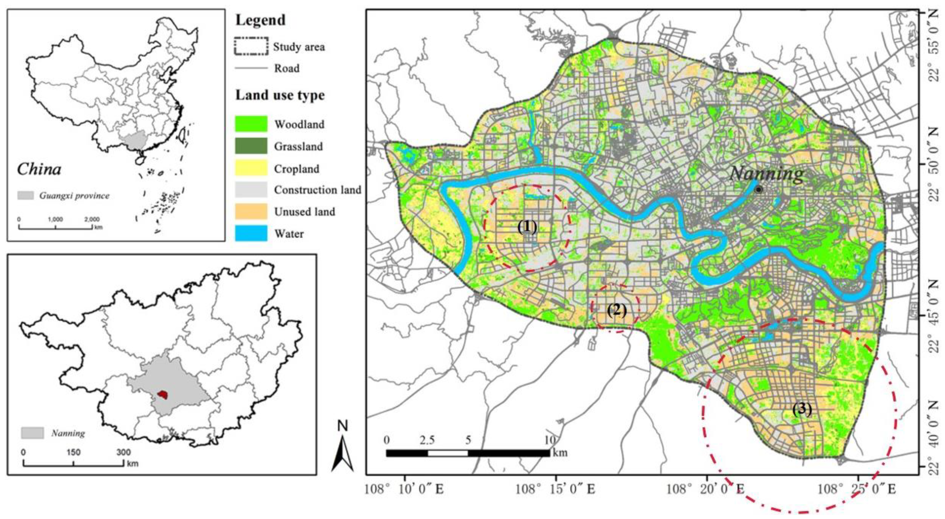
2.1. Study Area
2.2. Data Sources
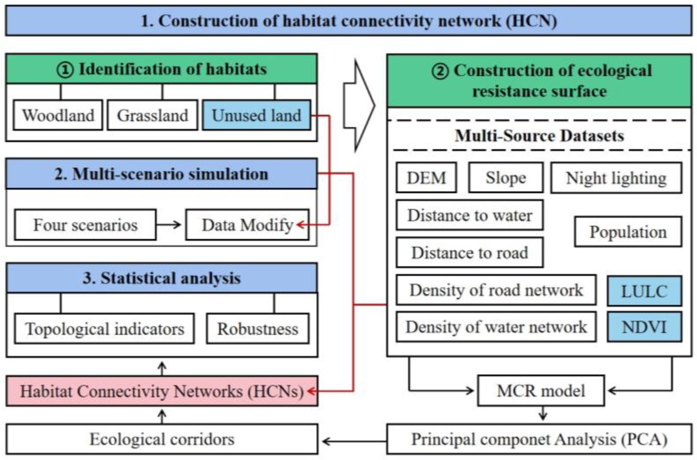
2.3. Methods
2.3.1. Selection of Habitats
2.3.2. Circuit Theory and MCR Model
2.3.3. Principal Component Analysis
2.3.4. Multiple Scenario Simulation
2.3.5. Topological Indicators for Evaluating HCNs
Average Degree
Diameter
Modularity
Clustering Coefficient
Eigenvector Centrality
Average Path Length
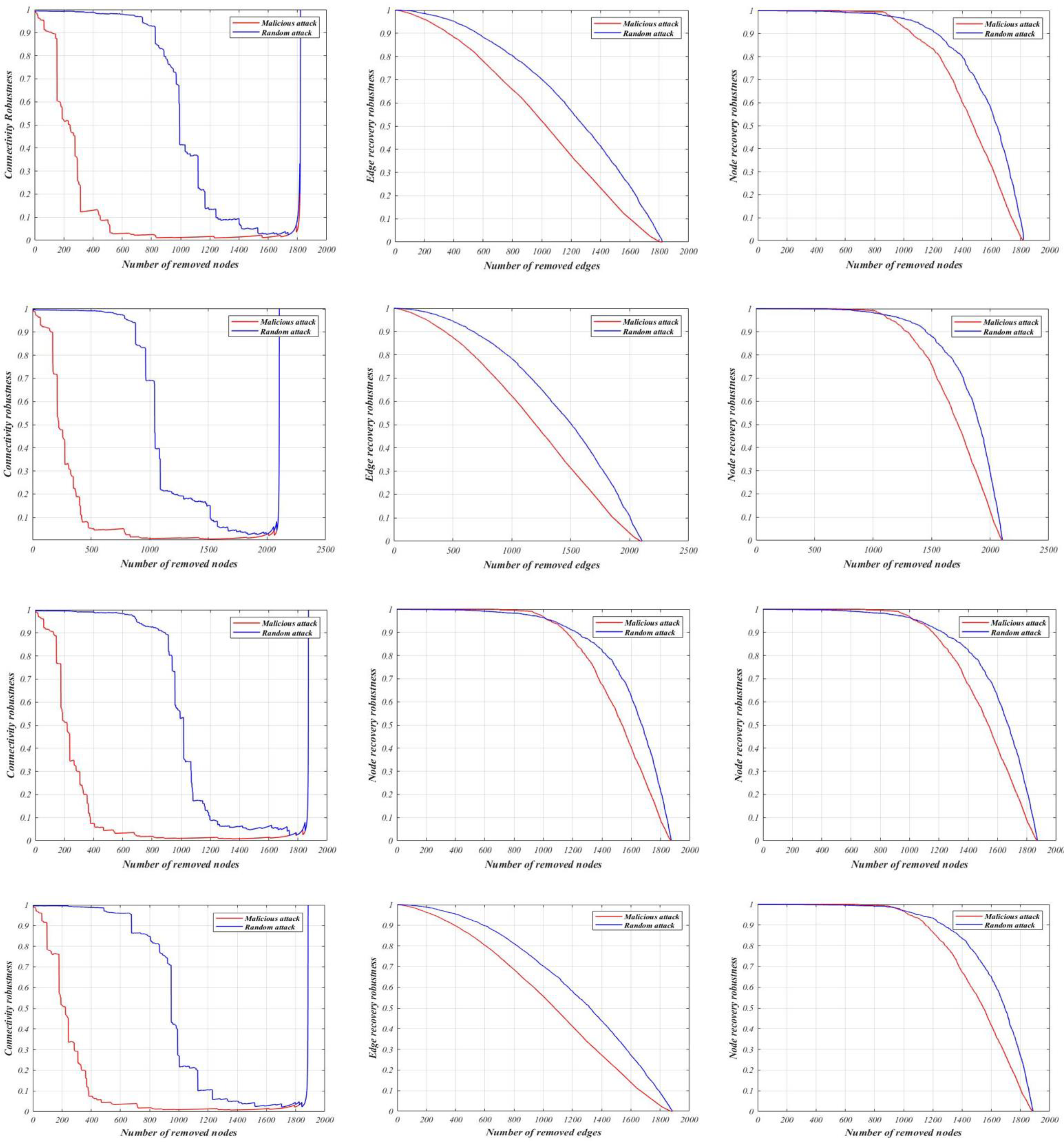
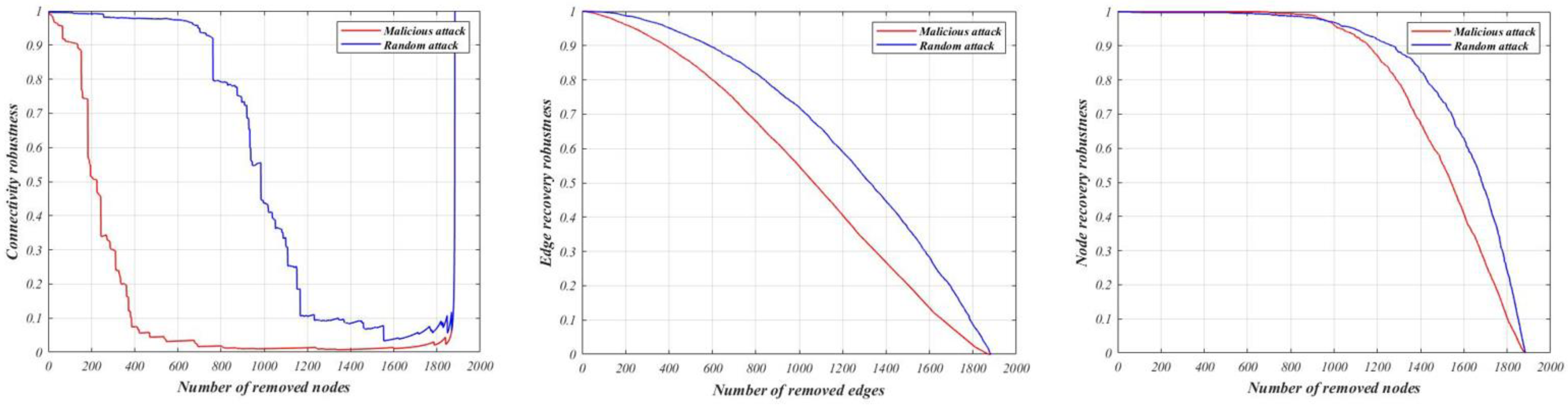
2.3.6. Robustness for Evaluating HCNs
3. Results
3.1. Spatial Distribution of Habitats
3.2. Principal Component Analysis and Minimum Cumulative Resistance Surface Analysis
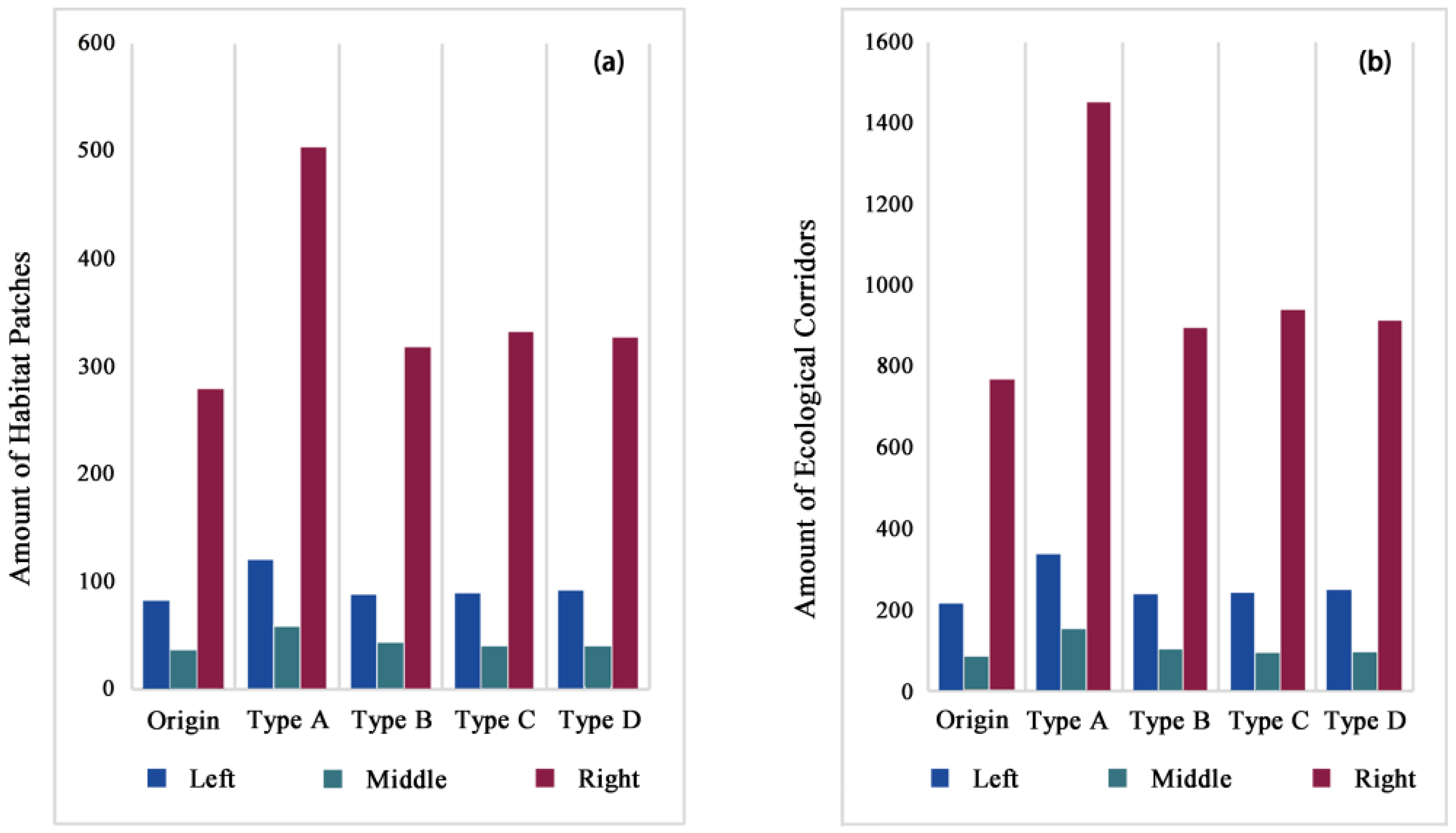
3.3. Analysis of HCNs
3.4. Topological Indicators Analysis of HCNs
3.5. Robustness Analysis of HCNs
4. Discussion
4.1. Construction of HCNs
4.2. Urban Expansion and the HCNs
4.3. Implications for Management
4.4. Limitations and Future Research Directions
5. Conclusions
Author Contributions
Funding
Data Availability Statement
Acknowledgments
Conflicts of Interest
References
- Grimm, N.B.; Faeth, S.H.; Golubiewski, N.E.; Redman, C.L.; Wu, J.; Bai, X.; Briggs, J.M. Global change and the ecology of cities. Science 2008, 319, 756–760. [Google Scholar] [CrossRef] [PubMed]
- Scolozzi, R.; Geneletti, D. A multi-scale qualitative approach to assess the impact of urbanization on natural habitats and their connectivity. Environ. Impact Assess. Rev. 2012, 36, 9–22. [Google Scholar] [CrossRef]
- Madadi, H.; Moradi, H.; Soffianian, A.; Salmanmahiny, A.; Senn, J.; Geneletti, D. Degradation of natural habitats by roads: Comparing land-take and noise effect zone. Environ. Impact Assess. Rev. 2017, 65, 147–155. [Google Scholar] [CrossRef]
- Chen, Y.; Rasool, M.A.; Hussain, S.; Meng, S.; Yao, Y.; Wang, X.; Liu, Y. Bird community structure is driven by urbanization level, blue-green infrastructure configuration and precision farming in Taizhou, China. Sci. Total Environ. 2023, 859, 160096. [Google Scholar] [CrossRef] [PubMed]
- Li, D.; Yang, Y.; Xia, F.; Sun, W.; Li, X.; Xie, Y. Exploring the influences of different processes of habitat fragmentation on ecosystem services. Landsc. Urban Plan. 2022, 227, 104544. [Google Scholar] [CrossRef]
- Li, G.; Fang, C.; Li, Y.; Wang, Z.; Sun, S.; He, S.; Qi, W.; Bao, C.; Ma, H.; Fan, Y.; et al. Global impacts of future urban expansion on terrestrial vertebrate diversity. Nat. Commun. 2022, 13, 1628. [Google Scholar] [CrossRef]
- Almenar, J.B.; Bolowich, A.; Elliot, T.; Geneletti, D.; Sonnemann, G.; Rugani, B. Assessing habitat loss, fragmentation and ecological connectivity in Luxembourg to support spatial planning. Landsc. Urban Plan. 2019, 189, 335–351. [Google Scholar] [CrossRef]
- Cisneros-Araujo, P.; Ramirez-Lopez, M.; Juffe-Bignoli, D.; Fensholt, R.; Muro, J.; Mateo-Sánchez, M.C.; Burgess, N.D. Remote sensing of wildlife connectivity networks and priority locations for conservation in the Southern Agricultural Growth Corridor (SAGCOT) in Tanzania. Remote Sens. Ecol. Conserv. 2021, 7, 430–444. [Google Scholar] [CrossRef]
- Fletcher, R.J., Jr.; Didham, R.K.; Banks-Leite, C.; Barlow, J.; Ewers, R.M.; Rosindell, J.; Holt, R.D.; Gonzalez, A.; Pardini, R.; Damschen, E.I. Is habitat fragmentation good for biodiversity? Biol. Conserv. 2018, 226, 9–15. [Google Scholar] [CrossRef]
- Lynch, A.J. Creating effective urban greenways and stepping-stones: Four critical gaps in habitat connectivity planning research. J. Plan. Lit. 2019, 34, 131–155. [Google Scholar] [CrossRef]
- Tarabon, S.; Bergès, L.; Dutoit, T.; Isselin-Nondedeu, F. Maximizing habitat connectivity in the mitigation hierarchy. A case study on three terrestrial mammals in an urban environment. J. Environ. Manag. 2019, 243, 340–349. [Google Scholar] [CrossRef] [PubMed]
- Kong, F.; Yin, H.; Nakagoshi, N.; Zong, Y. Urban green space network development for biodiversity conservation: Identification based on graph theory and gravity modeling. Landsc. Urban Plan. 2010, 95, 16–27. [Google Scholar] [CrossRef]
- Qian, M.; Huang, Y.; Cao, Y.; Wu, J.; Xiong, Y. Ecological network construction and optimization in Guangzhou from the perspective of biodiversity conservation. J. Environ. Manag. 2023, 336, 117692. [Google Scholar] [CrossRef] [PubMed]
- Forman, R.T.; Godron, M. Patches and structural components for a landscape ecology. BioScience 1981, 31, 733–740. [Google Scholar] [CrossRef]
- Fang, X.; Zhang, Y.; Xiang, Y.; Zou, J.; Li, X.; Hao, C.; Wang, J. A spatial model for coastal flood susceptibility assessment using the 2D-SPR method with complex network theory: A case study of a reclamation island in Zhoushan, China. Environ. Impact Assess. Rev. 2023, 98, 106953. [Google Scholar] [CrossRef]
- Huang, J.; He, J.; Liu, D.; Li, C.; Qian, J. An ex-post evaluation approach to assess the impacts of accomplished urban structure shift on landscape connectivity. Sci. Total Environ. 2018, 622, 1143–1152. [Google Scholar] [CrossRef]
- Albert, C.H.; Rayfield, B.; Dumitru, M.; Gonzalez, A. Applying network theory to prioritize multispecies habitat networks that are robust to climate and land-use change. Conserv. Biol. 2017, 31, 1383–1396. [Google Scholar] [CrossRef]
- Keeley, A.T.H.; Ackerly, D.D.; Cameron, D.R.; Heller, N.E.; Huber, P.R.; Schloss, C.A.; Thorne, J.H.; Merenlender, A.M. New concepts, models, and assessments of climate-wise connectivity. Environ. Res. Lett. 2018, 13, 073002. [Google Scholar] [CrossRef]
- Guo, H.; Yu, Q.; Pei, Y.; Wang, G.; Yue, D. Optimization of landscape spatial structure aiming at achieving carbon neutrality in desert and mining areas. J. Clean. Prod. 2021, 322, 129156. [Google Scholar] [CrossRef]
- Su, K.; Yu, Q.; Yue, D.; Zhang, Q.; Yang, L.; Liu, Z.; Niu, T.; Sun, X. Simulation of a forest-grass ecological network in a typical desert oasis based on multiple scenes. Ecol. Model. 2019, 413, 108834. [Google Scholar] [CrossRef]
- Dai, L.; Liu, Y.; Luo, X. Integrating the MCR and DOI models to construct an ecological security network for the urban agglomeration around Poyang Lake, China. Sci. Total Environ. 2021, 754, 141868. [Google Scholar] [CrossRef]
- Lee, K.M.; Kim, J.Y.; Cho, W.K.; Goh, K.I.; Kim, I.M. Correlated multiplexity and connectivity of multiplex random networks. New J. Phys. 2012, 14, 033027. [Google Scholar] [CrossRef]
- Zhou, D.; Elmokashfi, A. Network recovery based on system crash early warning in a cascading failure model. Sci. Rep. 2018, 8, 7443. [Google Scholar] [CrossRef]
- Podobnik, B.; Lipic, T.; Horvatic, D.; Majdandzic, A.; Bishop, S.R.; Eugene Stanley, H. Predicting the lifetime of dynamic networks experiencing persistent random attacks. Sci. Rep. 2015, 5, 14286. [Google Scholar] [CrossRef] [PubMed]
- Zhou, M.; Liu, J. A memetic algorithm for enhancing the robustness of scale-free networks against malicious attacks. Phys. A Stat. Mech. Its Appl. 2014, 410, 131–143. [Google Scholar] [CrossRef]
- Ramesh, A.; Satyavani, N. Seismic Image Enhancement from Principal Component Analysis: A Case Study from KG Basin. J. Geol. Soc. India 2022, 98, 1547–1552. [Google Scholar] [CrossRef]
- Qiu, S.; Yu, Q.; Niu, T.; Fang, M.; Guo, H.; Liu, H.; Li, S. Study on the Landscape Space of Typical Mining Areas in Xuzhou City from 2000 to 2020 and Optimization Strategies for Carbon Sink Enhancement. Remote Sens. 2022, 14, 4185. [Google Scholar] [CrossRef]
- Wang, L.; Wang, S.; Liang, X.; Jiang, X.; Wang, J.; Li, C.; Chang, S.; You, Y.; Su, K. How to Optimize High-Value GEP Areas to Identify Key Areas for Protection and Restoration: The Integration of Ecology and Complex Networks. Remote Sens. 2023, 15, 3420. [Google Scholar] [CrossRef]
- Shi, Y.; Zhang, K.; Li, Q.; Liu, X.; He, J.S.; Chu, H. Interannual climate variability and altered precipitation influence the soil microbial community structure in a Tibetan Plateau grassland. Sci. Total Environ. 2020, 714, 136794. [Google Scholar] [CrossRef] [PubMed]
- Fahrig, L. Ecological responses to habitat fragmentation per se. Annu. Rev. Ecol. Evol. Syst. 2017, 48, 1–23. [Google Scholar] [CrossRef]
- Marini, L.; Bartomeus, I.; Rader, R.; Lami, F. Species–habitat networks: A tool to improve landscape management for conservation. J. Appl. Ecol. 2019, 56, 923–928. [Google Scholar] [CrossRef]
- Von Haaren, C.; Reich, M. The German way to greenways and habitat networks. Landsc. Urban Plan. 2006, 76, 7–22. [Google Scholar] [CrossRef]
- Blair, R.B.; Johnson, E.M. Suburban habitats and their role for birds in the urban–rural habitat network: Points of local invasion and extinction? Landsc. Ecol. 2008, 23, 1157–1169. [Google Scholar] [CrossRef]
- Saura, S.; Bodin, Ö.; Fortin, M.J. Editor’S Choice: Stepping stones are crucial for species’ long-distance dispersal and range expansion through habitat networks. J. Appl. Ecol. 2014, 51, 171–182. [Google Scholar] [CrossRef]
- Hofman, M.P.; Hayward, M.W.; Kelly, M.J.; Balkenhol, N. Enhancing conservation network design with graph-theory and a measure of protected area effectiveness: Refining wildlife corridors in Belize, Central America. Landsc. Urban Plan. 2018, 178, 51–59. [Google Scholar] [CrossRef]
- Li, F.; Ye, Y.; Song, B.; Wang, R. Evaluation of urban suitable ecological land based on the minimum cumulative resistance model: A case study from Changzhou, China. Ecol. Model. 2015, 318, 194–203. [Google Scholar] [CrossRef]
- Grafius, D.R.; Corstanje, R.; Harris, J.A. Linking ecosystem services, urban form and green space configuration using multivariate landscape metric analysis. Landsc. Ecol. 2018, 33, 557–573. [Google Scholar] [CrossRef] [PubMed]
- Sandström, U.G.; Angelstam, P.; Mikusiński, G. Ecological diversity of birds in relation to the structure of urban green space. Landsc. Urban Plan. 2006, 77, 39–53. [Google Scholar] [CrossRef]
- Devictor, V.; Julliard, R.; Couvet, D.; Lee, A.; Jiguet, F. Functional homogenization effect of urbanization on bird communities. Conserv. Biol. 2007, 21, 741–751. [Google Scholar] [CrossRef]
- Yi, X.; Jue, W.; Huan, H. Does economic development bring more livability? Evidence from Jiangsu Province, China. J. Clean. Prod. 2021, 293, 126187. [Google Scholar] [CrossRef]
- Chace, J.F.; Walsh, J.J. Urban effects on native avifauna: A review. Landsc. Urban Plan. 2006, 74, 46–69. [Google Scholar] [CrossRef]
- Grunewald, K.; Bastian, O.; Louda, J.; Arcidiacono, A.; Brzoska, P.; Bue, M.; Cetin, N.; Dworczyk, C.; Dubova, L.; Fitch, A.; et al. Lessons learned from implementing the ecosystem services concept in urban planning. Ecosyst. Serv. 2021, 49, 101273. [Google Scholar] [CrossRef]
- Mitchell, M.G.; Bennett, E.M.; Gonzalez, A. Linking landscape connectivity and ecosystem service provision: Current knowledge and research gaps. Ecosystems 2013, 16, 894–908. [Google Scholar] [CrossRef]
- Liao, Z.; Su, K.; Jiang, X.; Wang, J.; You, Y.; Wang, L.; Chang, S.; Wei, C.; Zhang, Y.; Li, C. Spatiotemporal variation and coupling of grazing intensity and ecosystem based on four quadrant model on the Inner Mongolia. Ecol. Indic. 2023, 152, 110379. [Google Scholar] [CrossRef]
- Yu, Z.; Chen, L.; Li, L.; Zhang, T.; Yuan, L.; Liu, R.; Wang, Z.; Zang, J.; Shi, S. Spatiotemporal characterization of the urban expansion patterns in the Yangtze River Delta region. Remote Sens. 2021, 13, 4484. [Google Scholar] [CrossRef]
- Rimal, B.; Sloan, S.; Keshtkar, H.; Sharma, R.; Rijal, S.; Shrestha, U.B. Patterns of historical and future urban expansion in Nepal. Remote Sens. 2020, 12, 628. [Google Scholar] [CrossRef]
- Feng, R.; Wang, K. The direct and lag effects of administrative division adjustment on urban expansion patterns in Chinese mega-urban agglomerations. Land Use Policy 2022, 112, 105805. [Google Scholar] [CrossRef]
- Dhanaraj, K.; Angadi, D.P. Analysis of urban expansion patterns through landscape metrics in an emerging metropolis of Mangaluru Community Development Block, India, During 1972–2018. J. Indian Soc. Remote Sens. 2022, 50, 1855–1870. [Google Scholar] [CrossRef]
- Jezzini, N.; Nassif, N.; Mereu, V.; Faour, G.; Hassoun, G.; Mulas, M. Land Suitability Analysis for Forests in Lebanon as a Tool for Informing Reforestation under Climate Change Conditions. Forests 2023, 14, 1893. [Google Scholar] [CrossRef]
- Cuesta, F.; Calderón-Loor, M.; Rosero, P.; Miron, N.; Sharf, A.; Proaño-Castro, C.; Andrade, F. Mapping Above-Ground Carbon Stocks at the Landscape Scale to Support a Carbon Compensation Mechanism: The Chocó Andino Case Study. Forests 2023, 14, 1903. [Google Scholar] [CrossRef]
- Zhang, L.; Zhu, L.; Li, Y.; Zhu, W.; Chen, Y. Maxent modelling predicts a shift in suitable habitats of a subtropical evergreen tree (Cyclobalanopsis glauca (Thunberg) Oersted) under climate change scenarios in China. Forests 2022, 13, 126. [Google Scholar] [CrossRef]
- Alvey, A.A. Promoting and preserving biodiversity in the urban forest. Urban For. Urban Green. 2006, 5, 195–201. [Google Scholar] [CrossRef]


| Dataset | Time | Resolution | Data Sources (Accessed on 1 October 2022) |
|---|---|---|---|
| DEM | 2020 | 30 m | Download from NESSDC (http://www.geodata.cn/) |
| Night lighting | 2021 | 30 m | Download from NESSDC (http://www.geodata.cn/) |
| Sentinel-2 | 2020 | 10 m | Download from USGS (https://earthexplorer.usgs.gov/) |
| Population | 2020 | 30 m | Download from NESSDC (http://www.geodata.cn/) |
| Road | 2020 | 30 m | Download from NESSDC (http://www.geodata.cn/) |
| Water | 2020 | 30 m | Download from NESSDC (http://www.geodata.cn/) |
| DEM | 2020 | 30 m | Download from NESSDC (http://www.geodata.cn/) |
| Ecological Resistance Factor | 1 | 2 | 3 | 4 | 5 |
|---|---|---|---|---|---|
| DEM | ≤75 | (75, 100] | (100, 125] | (125, 150] | ≥150 |
| Slope (°) | ≤5 | (5, 10] | (10, 20] | (20, 30] | ≥30 |
| LULC | Woodland | Grassland | Cropland | Water | Building land |
| Night lighting | ≤45 | (45, 50] | (50, 55] | (55, 60] | ≥60 |
| NDVI | >0.45 | (0.4, 0.45] | (0.35, 0.4] | (0.3, 0.35] | ≤0.3 |
| Population | ≤1000 | (1000, 3500] | (3500, 6000] | (6000, 8500] | ≥8500 |
| Distance to road (m) | >400 | (300, 400] | (200, 300] | (100, 200] | ≤100 |
| Distance to water source (m) | ≥600 | (450, 600] | (300, 450] | (150, 300] | ≤150 |
| Density of the road network | ≤450 | (450, 800] | (800, 1150] | (1150, 1500] | ≥1500 |
| Density of the water network | ≤5 | (5, 10] | (10, 15] | (15, 20] | ≥20 |
| Amount/Type | Current | Scenario A | Scenario B | Scenario C | Scenario D |
|---|---|---|---|---|---|
| Habitat patches | 1822 | 2106 | 1873 | 1886 | 1884 |
| Ecological corridors | 5337 | 6235 | 5527 | 5564 | 5548 |
| Topological Indicator | Average Degree | Diameter | Modularity | Clustering Coefficient | Eigenvector Centrality | Average Path Length | |
|---|---|---|---|---|---|---|---|
| Current | western | 5.284 | 9 | 0.585 | 0.523 | 0.012 | 3.884 |
| central | 4.882 | 5 | 0.480 | 0.583 | 0.002 | 2.656 | |
| eastern | 5.551 | 12 | 0.718 | 0.544 | 0.036 | 5.405 | |
| Scenario A | western | 5.647 | 9 | 0.648 | 0.508 | 0.018 | 4.301 |
| central | 5.393 | 6 | 0.529 | 0.541 | 0.005 | 3.003 | |
| eastern | 5.776 | 14 | 0.763 | 0.515 | 0.069 | 6.347 | |
| Scenario B | western | 2.736 | 9 | 0.617 | 0.509 | 0.011 | 4.040 |
| central | 5.050 | 6 | 0.497 | 0.568 | 0.004 | 2.903 | |
| eastern | 5.652 | 12 | 0.723 | 0.523 | 0.044 | 5.69 | |
| Scenario C | western | 5.432 | 9 | 0.615 | 0.525 | 0.011 | 4.016 |
| central | 4.947 | 6 | 0.480 | 0.570 | 0.004 | 2.898 | |
| eastern | 5.673 | 13 | 0.722 | 0.518 | 0.046 | 5.839 | |
| Scenario D | western | 5.451 | 9 | 0.621 | 0.533 | 0.013 | 4.021 |
| central | 4.895 | 6 | 0.474 | 0.603 | 0.003 | 2.770 | |
| eastern | 5.618 | 12 | 0.736 | 0.541 | 0.043 | 5.627 | |
Disclaimer/Publisher’s Note: The statements, opinions and data contained in all publications are solely those of the individual author(s) and contributor(s) and not of MDPI and/or the editor(s). MDPI and/or the editor(s) disclaim responsibility for any injury to people or property resulting from any ideas, methods, instructions or products referred to in the content. |
© 2023 by the authors. Licensee MDPI, Basel, Switzerland. This article is an open access article distributed under the terms and conditions of the Creative Commons Attribution (CC BY) license (https://creativecommons.org/licenses/by/4.0/).
Share and Cite
Chang, S.; Su, K.; Jiang, X.; You, Y.; Li, C.; Wang, L. Impacts and Predictions of Urban Expansion on Habitat Connectivity Networks: A Multi-Scenario Simulation Approach. Forests 2023, 14, 2187. https://doi.org/10.3390/f14112187
Chang S, Su K, Jiang X, You Y, Li C, Wang L. Impacts and Predictions of Urban Expansion on Habitat Connectivity Networks: A Multi-Scenario Simulation Approach. Forests. 2023; 14(11):2187. https://doi.org/10.3390/f14112187
Chicago/Turabian StyleChang, Shihui, Kai Su, Xuebing Jiang, Yongfa You, Chuang Li, and Luying Wang. 2023. "Impacts and Predictions of Urban Expansion on Habitat Connectivity Networks: A Multi-Scenario Simulation Approach" Forests 14, no. 11: 2187. https://doi.org/10.3390/f14112187