Article

An Analysis of the Factors Affecting Forest Mortality and Research on Forecasting Models in Southern China: A Case Study in Zhejiang Province

1
State Key Laboratory of Subtropical Silviculture, Zhejiang A&F University, Lin’an 311300, China
2
Zhejiang Province Key Think Tank: Institute of Ecological Civilization, Zhejiang A&F University, Lin’an 311300, China
3
Key Laboratory of Carbon Cycling in Forest Ecosystems and Carbon Sequestration of Zhejiang Province, Zhejiang A&F University, Lin’an 311300, China
4
School of Environmental and Resources Science, Zhejiang A&F University, Lin’an 311300, China
5
College of Forestry, Fujian Agriculture and Forestry University, Fuzhou 350002, China
6
Zhejiang Forest Resources Monitoring Center, Hangzhou 310020, China
*
Author to whom correspondence should be addressed.
These authors contributed equally to this work.
Forests 2023, 14(11), 2199; https://doi.org/10.3390/f14112199
Submission received: 9 October 2023 / Revised: 28 October 2023 / Accepted: 2 November 2023 / Published: 6 November 2023
(This article belongs to the Section Forest Inventory, Modeling and Remote Sensing)

Abstract

:
Forests play a crucial role as the primary sink for greenhouse gases, and forest mortality significantly impacts the carbon sequestration capacity of forest ecosystems. A single type of forest mortality model has been developed, and its model variables are incomplete, leading to significant bias in mortality prediction. To address this limitation, this study harnessed data collected from 773 permanent plots situated in Zhejiang Province, China, spanning a period from 2009 to 2019. The primary objectives were to pinpoint the key variables influencing forest mortality and to construct forest mortality prediction models utilizing both traditional regression methods and machine learning techniques, ultimately aiming to provide a theoretical basis for forest management practices and future predictions. Four basic linear regression models were used in this study: Linear Regression (LR), Akaike Information Criterion (AIC) Stepwise Regression, Ridge Regression, and Lasso Regression. Four machine learning models, Gradient Boosting Regression (GBR), Random Forest (RF), Support Vector Regression (SVR), and Multilayer Perceptron (MLP), were used to model stand mortality. Mortality was used as the dependent variable, and environmental factors such as topographic factors, soil composition, stand characteristics, and climatic variables were used as independent variables. The findings unveiled that soil and stand-related factors exerted significant effects on the mortality rate, whereas terrain-related and climate factors did not exhibit statistical significance. The Random Forest model established by using stand age, tree height, ADBH, crown cover, humus layer thickness, and the biodiversity index has the highest fitting statistics such as R² and Mean Squared Error, indicating that it has a good fitting and prediction effect, which effectively predicts mortality at the stand level, and is a valuable tool for predicting changes in forest ecosystems, with practical value in estimating tree mortality to enhance forest management and planning.

1. Introduction

With the passage of time, the phenomenon of tree growth and death occurs one after another, and the stand changes accordingly. Tree mortality constitutes a central component of forest succession and dynamics, bearing significant importance for the population size, vegetation types, and distribution patterns of forest communities [1], which in turn affect the structure and function of tree populations. A quantitative analysis of tree mortality is very important for understanding the carbon storage, productivity, and dynamics of forests and can guide government workers to carry out forest protection work accurately [1,2,3]. Tree mortality can be quantified by generating tree mortality models, which provide reference for forestry decision making [4,5,6].
Forest mortality, a complex phenomenon, is subject to the influence of multiple endogenous and exogenous factors. Endogenous factors encompass individual trees, stand attributes, and human-induced disturbances, while exogenous factors comprise terrain, soil characteristics, climate conditions, wildfires, pest outbreaks, and geological disasters, among others. All of these factors significantly impact the natural mortality of trees [7]. Stand losses resulting from mortality events bring about alterations in population size, vegetation types, and distribution patterns within forest communities, thereby affecting the structure and functioning of tree species populations [8]. Analyzing forest biomass data stemming from both logging and natural mortality allows for the derivation of various indicators, including carbon storage and productivity, aiding in the assessment of their impact on forest communities [9]. However, current research endeavors lack regional and long-term continuous monitoring data on forest mortality, thereby hindering accurate assessments [10]. To build a more dependable tree mortality model and enhance the accuracy of future forest mortality predictions, this study obtained long-term reliable observational data.
Various modeling methods have been employed to develop single-tree and stand-level mortality models. Previous research has utilized traditional single-tree cumulative regression techniques to estimate the number of deceased trees [5,11,12], while logistic regression models [10,13] and mixed-effects models [14] have been used to determine the mortality rate of individual trees, which were then aggregated to obtain the total number of dead trees in a sample plot [15]. For instance, Zhang et al. derived a regression model for stand mortality using larch data from Northern China [15], and Li et al. proposed a series of regression models based on the Acadian Forest in North America [11]. Nevertheless, such estimation methods necessitate comprehensive single-tree information and tend to overlook model uncertainty [16,17]. By contrast, modelling stand-level mortality directly addresses these limitations. Previous studies have underscored the advantages of employing stand-level prediction models, emphasizing critical considerations in model selection and the choice of independent variables, asserting that mortality formulas should incorporate more detailed indicators such as tree species and terrain conditions at the stand level [18,19,20]. Furthermore, the integration of tree mortality with machine learning algorithms is relatively uncommon. Machine learning offers the ability to handle complex nonlinear relationships and high-dimensional data, enhancing the accuracy of tree mortality predictions and enabling adaptation to the intricate nature of forest ecosystems [21]. Thus, machine learning stands as a more flexible and efficient approach for calculating forest mortality compared to traditional statistical models. The aim of this study was to establish a genuine and precise stand-level mortality model by elucidating the relationship between factors and stand mortality; overcoming the aforementioned challenge; and employing various machine learning algorithms such as Random Forest, Gradient Enhanced Regression, Support Vector Regression, and Multi-layer Perceptron to construct a subtropical forest mortality model in China. The integration of these advanced modeling techniques significantly contributes to a deeper understanding of forest dynamics, culminating in more precise predictions and informed decisions concerning forest management and conservation efforts.
To address the aforementioned problems, this study selected four potential predictors: terrain variables, stand variables, soil variables, and climate variables. Traditional statistical methods and machine learning techniques were employed to construct a tree mortality model for Zhejiang Province. The specific objectives of this study are as follows: (1) To employ traditional statistical methods and machine learning techniques for selecting the optimal combination of predictive variables and establishing an accurate tree mortality model; (2) To develop a tree-based mortality model and evaluate its performance; (3) To assess the comprehensive predictors’ impact on tree mortality. The findings of this study hold relevance for large-scale forestry scenario analysis in actual regional management planning, thereby bearing significant importance for subtropical forest management planning and decision-making.

2. Study Areas and Methods

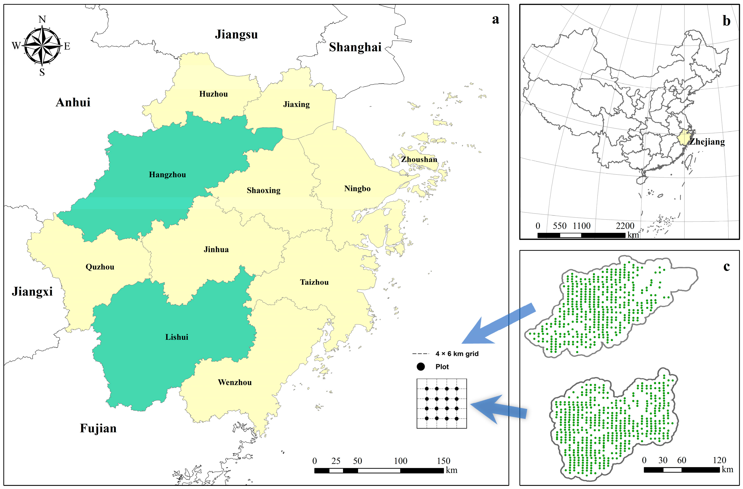
2.1. Description of Study Area

Data were gathered from 773 permanent plots distributed across close-to-nature forests in Hangzhou and Lishui, Zhejiang Province, Southern China (Figure 1). These permanent plots are systematic samples, evenly dispersed at 4 km × 6 km intervals on grid points based on the Beijing 54 coordinate system, with each plot comprising a square area of 800 square meters. The forests encompassed in these plots primarily consist of coniferous forests, broad-leaved forests, and mixed forests of evergreen broad-leaved species. There were 166 plots of coniferous pure forest (pure forest was a single tree species or the number of trees ≥ 90%), 40 plots of broad-leaved pure forest, and 567 mixed forests. There were 52 dominant tree species in the plot. These include Cupressus funebris, Sassafras tzumu, Liquidambar formosana, Pinus taeda, Castanopsis fargesii Franch, Castanopsis sclerophylla, Cryptomeria japonica var. sinensis, Quercus acutissima, Pinus massonian, Castanopsis carlesii, Schima superba, Phoebe zhennan, Alnus trabeculosa, Cyclobalanopsis glauca, Cunninghamia lanceolata Pinus elliottii, other soft woods, other hard woods, etc. This study collected data for two periods from 2009 to 2019.
We only included trees with a diameter at breast height (D) greater than 1 cm in our measurements of the number of trees, dominant species, average diameter at breast height (ADBH), average age, and crown cover. Traditionally, our starting threshold stood at 5 cm. However, we made an adjustment, lowering the initial threshold to 1 cm, with the aim of enhancing our capacity to assess the mortality of newly established trees.

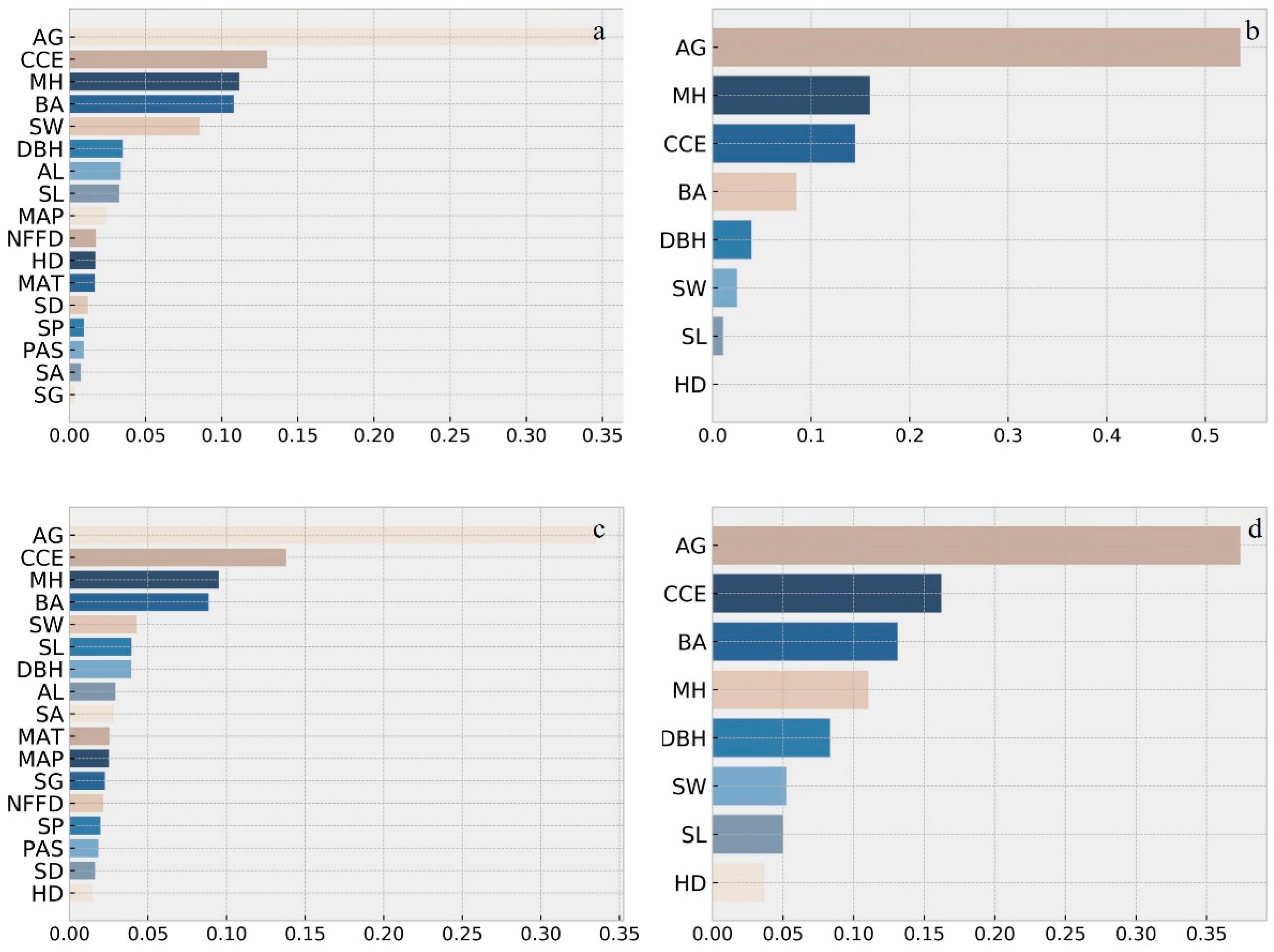
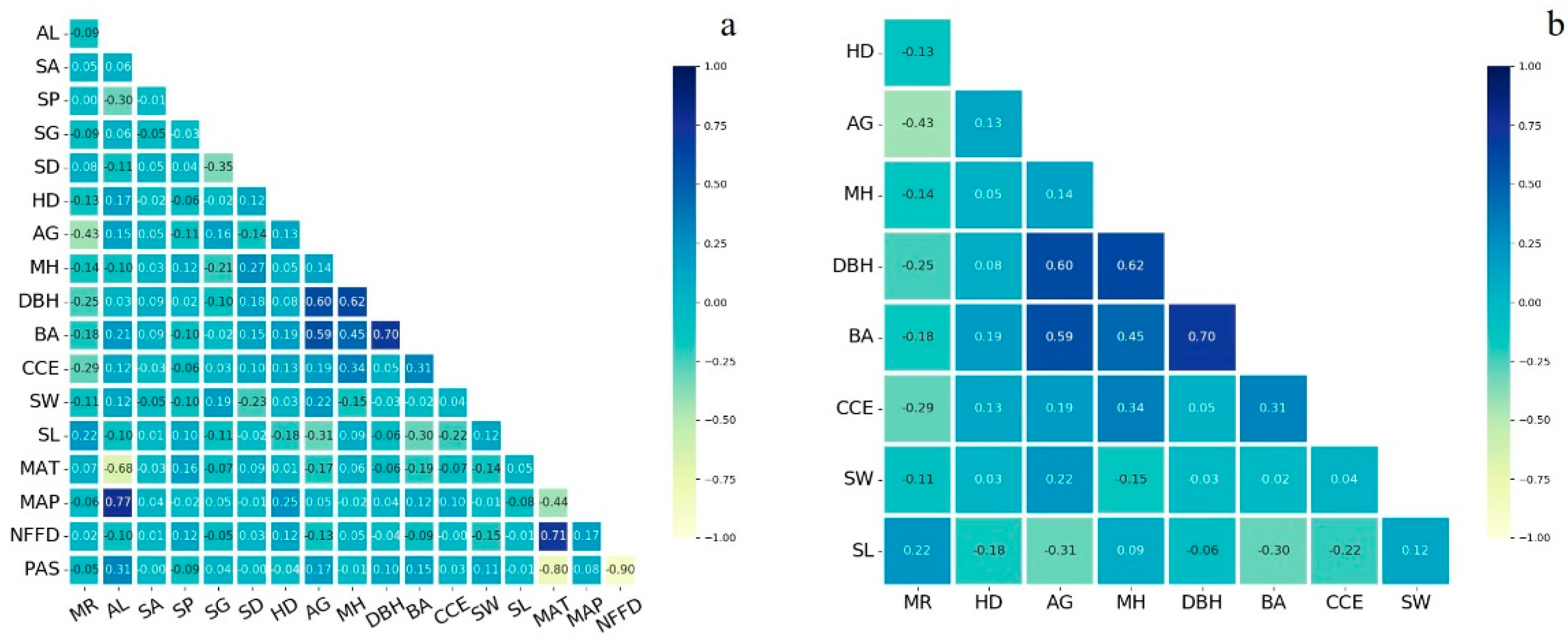
2.2. Selection of Predictor Variables

The selection of predictor variables in this study was a deliberate process, taking into careful consideration their ecological significance and observational relevance. It was essential to ensure that the chosen variables were not merely employed for statistical fitting but held biological relevance in elucidating the phenomena observed [10]. Drawing from sample plot investigations and relevant literature, we categorized all of the predictor variables, which we evaluated for their potential impact on tree mortality, into four sets based on their association with tree-, stand-, soil-, or climate-related mortality: (1) terrain predictor variables (T): altitude (AL), slope direction (SA), slope position (SP), and slope gradient(SG) [22,23]; (2) ground predictor variables (G): soil layer thickness (SD), humic layer thickness (HD) [24]; (3) stand predictor variables (S): the average age of forest stands (AG), average diameter at breast height (ADBH), stand dominant height (DH), basal area per hectare in forest stands (BA), Shannon–Wiener index (SW), Simpson’s index (SI), and crown cover extent (CCE) [25,26,27]; (4) climate predictor variables (C): average annual temperature(MAT), average annual rainfall (MAP), number of frost-free days (NFFD), and snowfall from August to July of the previous year (PAS) [24,28,29].
The AL of the sample points was determined using GPS and topographic maps. Virtual variables could also be set to multiple values if there were multiple states to ensure that the distance between the pairs was meaningful. For example, different directions could be set as 1 (east), 2 (west), 3 (south), and 4 (north). SA was assigned dummy variables ranging from −1 to 8 using the method proposed by Shao et al. Distribution refers to the slope at the north, northeast, east, southeast, south, southwest, west, northwest points and the flat slope. Similarly, the same method was applied to assign dummy variables to SP, ranging from 1 to 6 [30]. The average age of each dominant tree species constitutes the AG. ADBH was computed by measuring the average diameter at breast height of the dominant tree species in the main forest layer. Crown cover extent refers to the ratio of the canopy vertical projection coverage area to the plot area. The projection here is the vertical projection of the tree crown, which can be investigated via diagonal intercept sampling or visual survey method and recorded to two decimal places. When the crown cover extent was small (<0.4), the average canopy width method needed to be adopted; that is, the average canopy width area of the trees in the plot was multiplied by the number of trees to obtain the canopy coverage area and then divided by the plot area to obtain the crown cover extent or measured via diagonal intercept sampling. Soil variables were collected via field sampling. Climate datasets spanning from 2009 to 2019 were retrieved from the Climate AP database, based on the longitude, latitude, and elevation of each permanent sample plot. The Climate AP database is a national meteorological data repository that provides comprehensive information related to climate change, including vital parameters such as temperature, precipitation, wind speed, and various other meteorological metrics [31]. The data were derived from both extensive long-term observations and model-based estimates conducted at weather stations. The data acquisition interval was one year. For more detailed descriptions of these variables, see Table 1.

3. Models Selection and Approaches

3.1. Training Datasets

Our training dataset spans a period from 2009 to 2019 and encompasses a wide range of parameters related to trees, forests, soil, and climate. These parameters include AL, SA, SP, SG, SD, HD, AG, ADBH, DH, BA, SW, SI, CCE, MAT, MAP, NFFD, and PAS. In order to obtain these data, professional investigators conducted field surveys and sampling measurements to ensure the reliability and accuracy of the data. We collected a total of 76,070 observational data samples from different geographic regions and tree species to ensure the generalization performance of the model by screening for dead trees (trees that have died but not fallen) and live sample trees from 2009 to 2019.
Furthermore, about 100 samples were collected for each plot, and the mortality rate was calculated as a percentage of the total stock of dead trees in the forest. In the case of a relatively small forest area, forest mortality could also be expressed by calculating the number of dead trees as a percentage of the total number of trees in the forest. The tree mortality data within the training dataset exhibits a left-skewed distribution, with an average mortality rate of approximately 13%. This distribution suggests that most samples with low mortality rates correspond to areas with fewer tree fatalities, contributing to a relatively dispersed dataset.
The Linear Regression model employs random sampling to allocate 80% of the data for modeling, reserving the remaining 20% for validation. The training, validation, and testing set of machine learning follows an 8:1:1 ratio, using processed data to train and cross-validate specified models.

3.2. Linear Regression Models

We employed a selection of traditional Linear Regression, AIC Stepwise Regression, Ridge Regression, and Lasso Regression models to screen the predictors. Linear Regression primarily seeks to minimize the error between the actual value and the predicted value through the least squares method to identify the best predictors [32,33,34]. Stepwise Regression aims to maximize the predictive power of the model by identifying the optimal feature subset from a given set for feature selection [35,36]. Ridge Regression serves to reduce unnecessary features, simplifying the model and enhancing prediction accuracy [37,38]. Lasso Regression is particularly effective in addressing issues such as multicollinearity and overfitting [39,40].
We employed the Variance Inflation Factor (VIF) to address multicollinearity among predictors [41]. Predictors with VIF values less than 10 were retained in the final model, while variables with VIF values exceeding 10, such as MAT and NFFD, were excluded.
The Variance Inflation Factor (VIF) values for the two climate variables, MAT and NFFD, both exceed 10, signaling the presence of multicollinearity (Figure 2). By contrast, other topographic variables, soil variables, and stand variables do not exhibit multicollinearity. Three scenarios were analyzed: the removal of MAT alone, the removal of NFFD alone, and the simultaneous removal of both variables. Upon excluding NFFD from the analysis, we observed that the VIF values for the remaining 16 variables consistently remained below 10, indicating a rich dataset. However, when MAT alone was excluded, the VIF value for NFFD remained above 10. Consequently, we opted to remove NFFD.

3.3. Machine Learning Models

We opted for widely recognized machine learning algorithms, including Gradient Boosting Regression (GBR), Random Forest (RF), Support Vector Regression (SVR), and Multi-layer Perceptrons (MLP), to identify the most effective combinations of variables. The GBR algorithm excels in prediction accuracy by amalgamating multiple learning algorithms [42]. To enhance GBR’s performance, we carefully selected appropriate hyperparameters, including the number of learning algorithms (n_estimators = 2~3) and the number of nodes in the decision tree (max_depth = 20~100) [43]. In the RF algorithm, we optimized the number of randomly selected variables for decision tree nodes based on the specific number of independent variables, following the method proposed by Kuhn et al. [44]. With mortality as the dependent variable, we employed cross-validation, varying the number of randomly selected variables (mtry) from 1 to 17 using 10-fold cross-validation. We held the number of decision trees constant (ntrees = 600) and selected the variables that demonstrated the best generalization ability [45]. The SVM algorithm was sensitive to parameter and kernel function selection, necessitating specific adjustments for each problem [46]. We determined the best parameters through grid search using the training data and selected the optimal parameters for predicting mortality based on evaluation criteria. The range of the kernel functions considered included RBF, linear, and polynomial functions, while the regularization parameter (Cost) spanned from 1 to 20 [47]. For the MLP algorithm, we determined the number of hidden layers and the number of perceptrons in these hidden layers through iterative testing to achieve optimal performance [45]. We adopted the mean squared error (MSE) as the loss function and employed early stopping to prevent overfitting [48,49]. The optimal hyperparameters of the hidden layers were determined through grid search. We employed neural networks with these optimized parameters to predict stand mortality.

3.4. Data Structure

To explore the potential relationships between the independent variables and the dependent variables, we calculated the relative importance of the independent variables in the original dataset and their relative importance after some independent variables were removed for both the GBR model and RF model (Figure 3). Additionally, we examined the correlation between the original independent variables and the selected independent variables with higher importance (Figure 4).
In the original dataset, under the GBR model, the factors that significantly influenced the prediction of the mortality rate included AG, CCE, MH, BA, SW, ADBH, AL, SL, MAP, NFFD, HD, MAT, SD, SP, PAS, SA, and SG. Among these, AG, CCE, MH, and BA had relative importance scores exceeding 0.1. These four factors collectively contributed to 70% of the prediction, with the remaining factors having importance scores below 0.1. After reducing the number of independent variables to 8 based on their importance, the prominent predictors for predicting mortality rate remained AG, MH, CCE, BA, ADBH, SW, SL, and HD, with AG, MH, and BA accounting for up to 80% of the contribution, while the importance of the other variables remained below 0.1. Similarly, in the RF model, the key factors influencing the mortality rate in the original dataset were AG, CCE, MH, BA, SW, SL, ADBH, AL, SA, MAT, MAP, SG, NFFD, SP, PAS, SD, and HD, with AG and CCE having relative importance scores above 0.1. These two factors also contributed to 70% of the prediction, while the other factors had importance scores below 0.05. After reducing the importance of independent variables to 8, AG, CCE, BA, MH, ADBH, SW, SL, and HD emerged as the dominant predictors, with AG, CCE, and BA accounting for 70% of the contribution, and the importance of the other variables remaining below 0.1.
This analysis emphasizes the significance of several independent variables—AG, MH, CCE, BA, ADBH, SW, SL, and others—in predicting the target variables, making them pivotal considerations for subsequent analyses (Figure 3). While HD, a soil-related variable, may not be highly influential in the initial model that incorporates all 17 independent variables from the original dataset, it assumes significance in the Random Forest (RF) model following the screening of independent variables. Consequently, these eight independent variables wield substantial influence over the model’s performance and predictive capacity, offering potentially essential insights and explanatory power for achieving a high degree of accuracy in predicting the target variable. With the exception of HD, which is a soil factor, these variables pertain to stand factors, indicating that stand factors play the most substantial role in estimating the relative importance of independent and dependent variables and wield significant influence in model establishment. Among these independent variables, AG emerges as the most influential. This reinforces the idea that changes in stand age significantly affect tree mortality, with trees from different age groups displaying varying tolerance levels to environmental changes, consequently leading to diverse mortality rates. Conversely, the remaining nine independent variables exhibit lower importance in predicting the target variable. It is possible that these variables exert a weaker impact on the model’s performance and predictive capabilities, or their association with the target variable is less pronounced. During the process of model optimization or feature selection, the model may consider the exclusion of these lower-importance variables.
The heat map shows that the correlation between the stand factor and the dependent variable is relatively high (Figure 4). For example, stand ADBH and crown cover exhibit correlations of −0.25 and −0.29 with the mortality rate, ranking second only to the age factor. All other topographic factors, soil factors, and climate factors display absolute correlation values below 0.1, except HD, which has a correlation of −0.13. The factors with high correlation, namely AG, CCE, ADBH, and SL, align with the results of independent variable importance. AG and the mortality rate exhibit a negative correlation as high as −0.43. In the correlation between different independent variables, we observed that the correlation between topographic factors is not high. However, some topographic factors, such as AL, exhibit a notable correlation with climate factors like MAT and MAP, potentially due to altitude’s significant impact on climate. The correlation between stand factors is relatively strong, particularly with the mortality rate of the dependent variable, indicating interdependence or interaction among stand factors. Therefore, when establishing prediction models or conducting statistical analyses, it is advisable to consider the relationship between these related factors to avoid issues such as multicollinearity. The correlation between soil factors and other factors is not substantial, while the correlation between climate factors is high but not strongly correlated with the mortality rate of the dependent variable or other factors.
Data preprocessing for the data analysis methods was conducted in Excel 2016 (Microsoft, Redmond, WA, USA). Linear model construction and validation were performed using R 4.2.1 software (R Foundation for Statistical Computing, Vienna, Austria). Subsequently, machine learning models were built using Python 3.8. Relevant charts were created using Origin 2019b (OriginLab, Northampton, UK), and mapping was carried out using ArcMap 10.7 (Environmental Systems Research Institute, Redlands, CA, USA).

3.5. Model Evaluation

In this study, we employed three criteria to compare the goodness-of-fit of the models: the Akaike Information Criterion (AIC) [50], Bayesian Information Criterion (BIC) [51], and −2 times the value of the log-likelihood function (−2 logL). Smaller values of these criteria indicate a superior fit of the model to the data.
To assess the performance of the regression models, we employed five evaluation metrics: the coefficient of determination (R²), root mean square error (RMSE), mean absolute error (MAE), explained variance (EV), and accuracy. A higher R-squared value signifies a better alignment of the model with the data. Accuracy is a metric for the performance of classification models, measuring the proportion of correctly predicted samples out of the total samples. High accuracy indicates that the model is more reliable in making classification predictions. Conversely, lower values of MAE, MSE, and RMSE indicate a superior predictive performance of the model [52].
During the validation process of the machine learning models, we utilized cross-validation to assess their performance and generalization ability [53]. This technique involved dividing the dataset into multiple non-overlapping subsets, with each subset serving as a test set while the remaining subsets acted as training sets. Predictions were generated for each test set, and prediction errors were computed. Evaluation metrics such as RMSE and MAE were obtained through repeated cross-validation.

4. Results

4.1. Linear Regression Modelling Results

The fitting performance of each model (Table 2) and the fitting results of the model on the training dataset (Table 3) were derived from four distinct models: the Linear Regression model (M1), AIC Stepwise Regression model (M2), Ridge Regression model (M3), and Lasso Regression model (M4).
The results show that the AIC Stepwise Regression model (M2) had the second highest R² and relatively low AIC, BIC, and −2 logL values, indicating a better fitting performance. When selecting the optimal model, considering the practical application of the model, the AIC Stepwise Regression equation (M2) was more meaningful and involved fewer independent variables, which was favorable for simplifying the model operation and enhancing the applicability of the model. The Linear Regression model (M1) had the best performance in terms of R² and the smallest AIC and BIC. This indicates that the Linear Regression model was well suited to represent mortality data. On the contrary, the Ridge Regression model (M3) was poorly fitted, indicating that the Ridge Regression method was not suitable for capturing the underlying relationships in the mortality data. The Lasso Regression model (M4), with a smaller R² and larger −2 logL value, was also not suitable for fitting the mortality data.
The equation after AIC Stepwise Regression is as follows:
y = 0.5951 22.56 H D 141.20 A G 90.37 D B H + 51.80 B A 159.38 C C E + 46.33 S L
In this model, the independent variables AG, ADBH, BA, CCE, and SL exhibit significance. All of these factors are linked to the forest stand, underscoring their substantial influence in the predictive model and their pivotal role in predictive importance. The parameters for HD, AG, ADBH, and CCE are characterized by negative values, while the parameters for BA and SL are positive. The negative parameters for HD, AG, and ADBH imply that as HD and ADBH increase during tree growth, the mortality rate decreases. Younger trees are more susceptible to mortality, whereas mature forests experience lower mortality due to external factors and their inherent characteristics. The negative parameter for CCE suggests that enhanced canopy growth, quicker crown cover, and a larger canopy projection lead to lower annual mortality rates [27]. Conversely, the positive parameter for BA and SL indicates that higher basal area and stand density are associated with increased mortality rates, implying that forest overcrowding may result in elevated mortality.

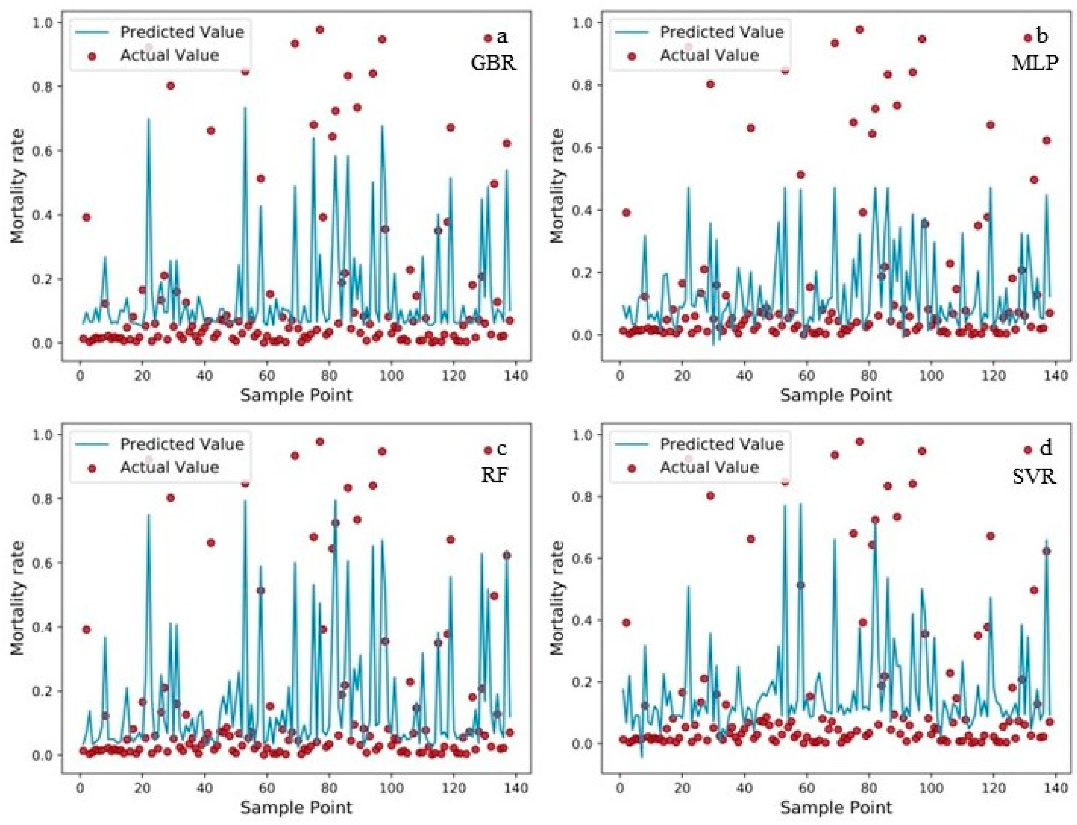
4.2. Machine Learning Modelling Results

To obtain the optimal model for fitting the mortality rate, this study compares the results of estimating the mortality rate using Random Forest (RF), Gradient Boosted Regression (GBR), Support Vector Regression (SVR), and Multi-Layer Perceptron (MLP) models. A comprehensive comparison of the accuracy of these four machine learning algorithms in estimating the mortality rate was conducted (Table 4 and Table 5).
A grid search algorithm was also employed to fine-tune the model hyperparameters and enhance overall prediction performance. Furthermore, adjusting the max_depth parameter and selecting the appropriate number of nodes led to improved data fitting. The new dataset, with feature dimensions reduced from 17 independent variables to eight independent variables while maintaining the sample size, significantly impacted the GBR and RF models. The n_estimators for the GBR and RF models under the new dataset were substantially reduced from 100 and 258 to 20 and 23, respectively. Notably, there was no significant change in the accuracy of the GBR and RF models in the source dataset. The RF model performed notably better in the new dataset, achieving the highest accuracy value of 63%. This suggests that the GBR and RF models under the new dataset achieve better fitting and prediction performance with fewer decision trees and computations. Additionally, it reveals that the features of terrain and climate in the source dataset have less influence on the model prediction.
For the RF model, its fitting accuracy increased with the number of decision trees, and once the number of decision trees surpassed a critical value, the model’s fitting accuracy stabilized. The Random Forest parameters set during grid search, such as the depth of the decision tree and the minimum number of samples split, were more complex compared to GBR [54]. The same setup results can be observed (Table 4). Regarding the SVR model, it employed various kernel functions (RBF, linear, and poly) and kernel coefficients (gamma ranging from 0.001 to 1) along with the penalty coefficient (cost ranging from 1 to 20). The optimal parameters were determined through grid search during training, using the fitted data. The SVR model selected RBF as the kernel function to accomplish nonlinear mapping during training. The cost parameter was set to five, indicating that the model was less penalized and more suitable for the size of the dataset, enhancing the model’s flexibility in predicting samples. The epsilon setting of 0.1 indicates that the fitting process of the training samples was more stringent. For the MLP model, it consisted of two hidden layers, each containing 16 neurons. The number of learning iterations was selected from an interval of (100, 200, 500), and 500 rounds were ultimately used as the number of iterations through grid search. This implies that a large number of repetitions were used to repeat the training and are more suitable for training the new dataset with the MLP fit. The learning rate was changed from 0.0001 to 0.1 in steps of 0.0005.
The sizes of fit statistics for different machine learning models are presented, including R-squared value (R²), mean squared error (MSE), explained variance score (EVS), mean absolute error (MAE), and accuracy (Table 6). Among the models, the Random Forest model stands out with a high fitting accuracy, achieving an R-squared value of more than 0.6. The GBR model also demonstrates a high fitting accuracy for the original dataset, with an R-squared value of 0.6198. This suggests that the GBR model performs well in handling a dataset with multiple features and intermixed redundant information. However, the SVR and MLP models show poor fitting conditions, indicating that they might not be the most suitable choices for this specific dataset and prediction task. It is worth noting that the coefficient of determination even increased after removing the low eigenvalue variables, indicating the robustness of the Random Forest model, which was therefore chosen as the best machine learning model for predicting mortality. In summary, the results (Table 6) substantiate the superior predictive capability of the Random Forest model in accurately forecasting mortality, with the Gradient Boosting Regression (GBR) model ranking as the next best performer in this regard.
The order of predictive performance can be observed as follows: the RF model, GBR model, SVR model, and MLP model (Figure 5). In our data analysis, we observed data points that deviate from the normal distribution trend of mortality rates and significantly affect the model’s fitting accuracy, treating them as outliers. Typically, mortality rates are distributed between 0 and 0.4. However, there are very few samples with mortality rates distributed between 0.8 and 1. The data distribution in this range significantly deviates from the values observed of most samples, not conforming to the growth patterns of sample trees in the study area. In analyzing the distribution of fitted values against actual values in the test set, it is evident that the RF model outperforms the other models. This superior performance is discerned through its capacity to maintain a more uniform distribution and effectively accommodate data points with elevated values. By contrast, the MLP model exhibits suboptimal performance, particularly in handling outliers. Notably, there is a substantial disparity between the fitted values and the actual values for data points with a mortality rate exceeding 0.46. Both the RF model and the GBR model demonstrate a heightened sensitivity to outliers, with the fitted values for high-mortality data points aligning more closely with their corresponding actual values. The SVR model, on the other hand, exhibits poor fitting for values with low mortality rates, whereas the RF model and MLP model provide a better fit for lower values. Additionally, it is noteworthy that all four model types tend to overpredict values approaching 0, especially the SVR model.
A smaller root mean square error (RMSE) indicates a closer alignment between the model’s predictions and the actual observed values, signifying a higher degree of predictive accuracy. Figure 6 reveals that the models perform more effectively with larger sample sizes and exhibit enhanced prediction accuracy when the mortality rate is less than 0.2, reflecting a relatively favorable mortality rate within the region. It is worth noting that, despite the majority of values for the dependent variable—mortality rate—falling within the range of (0, 0.2), the overall RMSE within this context spans from 0.155 to 0.181. This range suggests that the model experiences relatively minor prediction errors, indicating robust model performance and a heightened level of accuracy in forecasting actual values (Figure 6). When assessing the RMSE rankings, the models can be ordered as follows: RF model, GBR model, SVR model, and MLP model. Particularly, the RF model stands out as it exhibits the lowest RMSE, rendering it the most suitable model for the test set. It is worth noting that the predicted values for all four models tend to exceed the actual values when the mortality rate is less than 0.1, a pattern consistent with the observations (Figure 5). Conversely, when the mortality rate surpasses 0.4, the predicted values typically fall below the actual values. Given that only 11% of the samples have a mortality rate exceeding 0.4, the models naturally predict lower values for samples with high mortality rates, aligning with the data distribution.
The residual distribution of the models aligns with the previously discussed results (Figure S1): the RF model exhibits a better residual distribution compared to the other models, with the GBR and MLP models closely following suit, while the SVR model displays a low residual distribution. Residuals for all four models predominantly cluster within the range of (−2, 2). Specifically, the residual distribution of the RF model skews closer to a normal distribution, with the average of the residuals approaching zero, slightly on the negative side. Notably, the RF model exhibits a minimal number of outliers in the residuals, and there is no discernible evidence of heteroscedasticity or autocorrelation. By contrast, the residual distribution of the GBR and MLP models skews more negatively, indicating a model bias towards predicting values that are generally lower than the actual observed values. Furthermore, the GBR model exhibits fewer outliers in the residuals when compared to the MLP model, and like the RF model, it also exhibits an absence of signs of heteroscedasticity and autocorrelation. Conversely, the SVR model demonstrates a more pronounced negative bias in its residual distribution, suggesting a proclivity to predict values significantly lower than the actual observed values.

5. Discussion

In all models, the RF model consistently demonstrated the most robust predictive performance, which aligns with the findings reported by Zanella et al. [55]. The model has lower MAE and RMSE compared to other models. In addition, the optimization of the sampling and tree-building process greatly improves the training speed and accuracy of the results, and by capturing the non-linear relationships in the sample space, the RF model effectively overcomes the limitations of traditional statistical methods in mortality data analysis.
Studies have demonstrated the substantial influence of topographic factors, particularly altitude, on forest mortality. With rising altitude, there is a decrease in temperature, which can impact the suitability of certain tree species, ultimately leading to elevated mortality rates in these regions [56,57]. However, given that the permanent plots in this study were situated in the low mountains, hills, and plains of Zhejiang Province, China, where altitude and slope exhibit minimal variation, the optimal model did not incorporate altitude and slope as predictors. This observation suggests that elevation and slope factors exert no significant influence on stand mortality in this specific context.
On the other hand, soil factors were found to emerge as pivotal determinants of stand mortality, consistent with prior investigations [58]. Specifically, the thickness of the humus layer (HD) emerged as a significant variable in the modeling process. HD made a substantial contribution to the model’s overall importance and significantly influenced the formulation of the forest mortality model. Natural tree mortality is notably pronounced during the early stages of growth, when trees have heightened requirements for both light and substantial soil nutrient availability; therefore, HD assumes a critical role as a predictor in determining mortality rates.
The association between AG, ADBH and tree mortality was thoroughly examined. The findings revealed that with increasing stand age, there is a marked decrease in both the likelihood of stand mortality and the quantity of deceased trees within the stand. This outcome aligns with a study conducted on Wang et al.’s research on sample plots in the Jiangshanjiao experimental forestry site in Heilongjiang Province [59]. It underscores the existence of a negative link between AG, ADBH, and tree mortality, although such associations may vary, contingent upon the specific ecological context and forest typology [60]. However, the forests in the study area are divided into natural secondary forests and man-made managed forests with a relatively simple composition. The natural secondary forests primarily comprise a mixture of broad-leaved tree species, whereas the managed forests predominantly consist of pure stands of Chinese fir and pine. In view of the somewhat limited sample size, this study has chosen to amalgamate managed and natural forests to create a comprehensive, large-scale stand loss model that encompasses both tree mortality and tree age. Nonetheless, it is of paramount importance for future research endeavors to develop distinct models for managed and natural forests. These models should emphasize the increase in tree mortality with advancing age within natural forests and elucidate the specific circumstances under which younger trees in managed forests are more prone to mortality.
This study delves deeper into the impact of CCE on stand mortality. As CCE increased, both the probability of tree mortality and the number of deceased trees within the stand were observed to exhibit a significant reduction. This discovery aligns with the research conducted by Zhao et al., where it was documented that an augmentation in ADBH and CCE corresponded with a decline in the number of deceased trees [61]. Augmenting the canopy cover plays a pivotal role in regulating the microclimate within the stand. This regulation involves the provision of shade and the mitigation of temperature extremes, ultimately creating a more stable and conducive environment for tree growth and subsequently diminishing stress-induced mortality. Moreover, the dense canopy has the added advantage of retaining water in forest ecosystems by reducing evaporation and runoff [27]. This water retention significantly benefits tree roots, particularly during periods of drought, consequently mitigating mortality attributed to water stress. In addition, a dense canopy effectively minimizes direct sunlight access to the forest floor, thus reducing the competition for light among trees [25]. This, in turn, fosters the flourishing of understory trees and alleviates mortality stemming from insufficient light and shade. The outcomes of this study unequivocally demonstrate that denser canopies contribute to more favorable growing conditions for trees, resulting in a substantial reduction in stand mortality.
Moreover, forest density and BA emerged as additional pivotal factors exerting a substantial influence on stand mortality. Previous investigations conducted by Hallinger et al. and Moore et al. have put forth evidence suggesting that elevated stand density correlates with an increased likelihood of tree mortality within a given age and stand structure [23,62]. In a parallel vein, Palmas et al.’s research on natural mixed forests in Chile established models demonstrating that, as stand density approaches maximum density, the stand experiences augmented levels of mortality [63]. In this current study, the significance of BA as a predictor variable was also prominently featured. In this study, the importance of BA as a predictor variable was notably highlighted. This significance can be attributed to the extended, uninterrupted growth of permanent sample plots within the forest. These plots exhibit a spatial structure distribution closely resembling a natural distribution, thereby offering favorable growth conditions for this study.
Furthermore, this study delved into the relationship between climate factors and the likelihood of tree mortality. Global warming, drought, pests, and diseases can all cause tree deaths. Prolonged drought can kill trees, causing permanent damage to their water-carrying tissues. Trees susceptible to drought are more vulnerable to pests such as bark beetles and fungi [64]. The decrease in soil moisture levels due to rising temperatures is a major driver of tree mortality [65]. High temperatures also contribute to wildfires, especially in the Americas and Europe [66]. Subtropical forests are less likely to have forest fires due to natural causes in the same period of rain and heat, while the Mediterranean climate of Western North America and Europe has dry summers and less precipitation, resulting in national forests in the northern interior regions suffering large tree losses due to wildfires. In addition, climate change is likely to lead to an increase in natural tree deaths, which, unlike tree deaths caused by disturbance, will continue to decline from southern regions to the north, with forest mortality likely to follow as temperatures rise. Prior investigations by Zhang et al. have illustrated that as climate warms, the likelihood of tree mortality under water stress exhibits an upward trajectory [67]. When forests are subjected to major natural disasters such as fires, typhoons, and extreme climate such as extreme high temperature and extreme precipitation, a large area of trees will die. With respect to this prediction, the area of this current study is relatively inland, not coastal. In addition, between 2009 and 2019, it did not suffer major natural disasters and was not prone to extreme weather conditions that led to widespread tree deaths. Consequently, the findings of this study suggest that climate factors exerted no significant impact on tree mortality within the permanent plots of Zhejiang Province; therefore, the four climate factors assessed, MAT, MAP, NFFD, and PAS, were not encompassed within the optimal model. Nevertheless, in the context of long-term climate change, the 10-year time horizon may not capture the full impact of the climate change taking place on Earth, and longer time horizons should be studied in the future, taking into account the possible impact of other climate factors on tree death.
The study concentrated on analyzing terrain, soil, forest stand, and climate factors in the context of tree mortality. Nevertheless, it is important to acknowledge that the factors influencing forest mortality extend beyond these four categories. Exploring additional factors and their potential interactions could enhance the predictive capacity of the developed models. Forest mortality is a complex issue influenced by various factors, including biological elements such as insects, fungi, and wildlife. The study by Dudek and Grużewska in Northeastern Poland found that damage caused by wildlife herbivores takes precedence, followed by pathogenic fungi and insects, with the severity of damage dependent on the source, tree species, and age [68]. The research conducted by Kautz, Meddens, Hall, and Arneth explores the impact of biotic disturbances on forest ecosystems, emphasizing the significant influence of insects, particularly in northern hemisphere forests, akin to wildfires [69]. Furthermore, the study by Sierota, Grodzki, and Szczepkowski underscores the varying effects of biological factors on different tree species and ages [70]. In future regression model construction, it is crucial to comprehensively consider these factors to better explain variations in forest mortality. For instance, the discernible impact of air pollution on forest mortality is particularly pronounced in the temperate regions of Europe and Asia within the Northern Hemisphere. A comprehensive perspective on alterations in tree mortality due to air pollution can be gleaned by contrasting these regions with others in Europe and North America [71].
In forthcoming research endeavors, the greenhouse gas inventory report prepared by Suichang County will be employed to validate model outcomes. By integrating the finely calculated forest mortality rates into the formula used for computing carbon emissions arising from forest mortality biomass, a more precise evaluation of carbon emissions resulting from tree mortality can be achieved. This approach will prove invaluable for informing policy decisions pertaining to forest management and carbon sequestration, as it facilitates a deeper comprehension of the environmental repercussions of tree mortality and its potential implications for carbon emissions.

6. Conclusions

Forest ecosystems occupy a pivotal position in upholding equilibrium and steadiness within terrestrial ecosystems, and any increase in forest mortality can impart noteworthy repercussions on these intricate ecological systems. This investigation was primarily centered on the scrutiny of the determinants influencing stand mortality within subtropical forests situated in Zhejiang Province. Eight regression and machine learning models were constructed using four types of environmental variables to predict stand mortality in the tree populations of subtropical forests.
The research outcomes have successfully identified the pivotal factors that underlie stand mortality in subtropical regions. Furthermore, this study unequivocally established the superiority of the RF model in the domain of forecasting forest mortality within these specific areas. This model effectively integrates various stand characteristics, including AG, DH, CCE, and HD, thereby enabling more precise predictions of forest mortality. The newly developed stand-level mortality rate model exhibits exceptional statistical properties, making it highly suitable for inclusion in government greenhouse gas inventories and for conducting extensive calculations concerning carbon emissions resulting from forest mortality biomass.
In light of the ongoing global climate change, factors affecting tree mortality may become more frequent and intense. The results of this study show that the average rate of loss in forest stock volume in Zhejiang Province is currently 13.60 percent and will increase thereafter. There is an urgent need to enhance our comprehension of how trees respond to these mortality factors within ecosystems. Developing a deeper mechanistic understanding of the mortality process can lead to better process models for subtropical forest mortality and aid forest managers in implementing effective management practices to enhance forest quality and resilience in the face of a changing climate. This knowledge will play a pivotal role in adapting forest management strategies to address the uncertainties that lie ahead for forest ecosystems within the context of a warming climate.

Supplementary Materials

The following supporting information can be downloaded at: https://www.mdpi.com/article/10.3390/f14112199/s1, Figure S1: The figure shows the residual distribution of (a) GBR, (b) MLP, (c) RF and (d) SVR model test sets, respectively. The abscissa is the predicted value of the depletion rate, the ordinate is the standardized residual.

Author Contributions

Conceptualization: Z.D.; methodology: Z.D., B.J. and X.C.; software: Z.D. and X.S.; validation: H.Y. and S.Y.; formal analysis: Z.D. and B.J.; investigation: Z.D., X.C., S.L. and Y.S.; data curation: B.J. and H.Y.; writing—original draft: Z.D., X.C. and Y.S.; writing—review & editing: Z.D., B.J. and Y.S.; visualization: Z.D. and X.S.; supervision: Y.S.; project administration: Y.S.; resources: Z.D. and S.Y.; funding acquisition: L.X., Y.Z. and Y.S. All authors have read and agreed to the published version of the manuscript.

Funding

This research was funded by the Key Research and Development Program of Zhejiang Province (Grant number: 2023C02003; 2021C02005; 2022C03039); the Joint Research Fund of the Department of Forestry of Zhejiang Province and Chinese Academy of Forestry (Grant No. 2022SY05); the National Natural Science Foundation of China (Grant number: 32001315; U1809208; 31870618); and the Scientific Research Development Fund of Zhejiang A&F University (Grant number: 2020FR008).

Data Availability Statement

The raw/processed data required to reproduce these findings cannot be shared at this time as the data also form part of an ongoing study.

Conflicts of Interest

The authors declare no conflict of interest.

References

  1. Chambers, J.Q.; Higuchi, N.; Teixeira, L.M.; dos Santos, J.; Laurance, S.G.; Trumbore, S.E. Response of tree biomass and wood litter to disturbance in a Central Amazon forest. Oecologia 2004, 141, 596–611. [Google Scholar] [CrossRef] [PubMed]
  2. Liu, Q.; Peng, C.; Schneider, R.; Cyr, D.; McDowell, N.G.; Kneeshaw, D. Drought-induced increase in tree mortality and corresponding decrease in the carbon sink capacity of Canada’s boreal forests from 1970 to 2020. Glob. Chang. Biol. 2020, 29, 2274–2285. [Google Scholar] [CrossRef]
  3. Perez-Quezada, J.F.; Barichivich, J.; Urrutia-Jalabert, R.; Carrasco, E.; Aguilera, D.; Bacour, C.; Lara, A. Warming and Drought Weaken the Carbon Sink Capacity of an Endangered Paleoendemic Temperate Rainforest in South America. J. Geophys. Res. Biogeosci. 2023, 128, e2022JG007258. [Google Scholar] [CrossRef] [PubMed]
  4. Eid, T.; Tuhus, E. Models for individual tree mortality in Norway. For. Ecol. Manag. 2001, 154, 69–84. [Google Scholar] [CrossRef]
  5. Xie, L.; Chen, X.; Zhou, X.; Sharma, R.P.; Li, J. Developing Tree Mortality Models Using Bayesian Modeling Approach. Forests 2022, 13, 604. [Google Scholar] [CrossRef]
  6. Yao, X.; Titus, S.J.; Macdonald, S.E. A generalized logistic model of individual tree mortality for aspen, white spruce, and lodgepole pine in Alberta mixed wood forests. Can. J. For. Res. 2001, 31, 283–291. [Google Scholar]
  7. Cailleret, M.; Bircher, N.; Hartig, F.; Hülsmann, L.; Bugmann, H. Bayesian calibration of a growth-dependent tree mortality model to simulate the dynamics of European temperate forests. Ecol. Appl. Publ. Ecol. Soc. Am. 2020, 30, e02021. [Google Scholar] [CrossRef]
  8. Batllori, E.; Lloret, F.; Aakala, T.; Anderegg, W.R.L.; Aynekulu, E.; Bendixsen, D.P.; Bentouati, A.; Bigler, C.; Burk, C.J.; Camarero, J.J.; et al. Forest and woodland replacement patterns following drought-related mortality. Proc. Natl. Acad. Sci. USA 2020, 117, 29720–29729. [Google Scholar] [CrossRef]
  9. Lun, F.; Liu, Y.; He, L.; Yang, L.; Liu, M.; Li, W. Life cycle research on the carbon budget of the Larix principis-rupprechtii plantation forest ecosystem in North China. J. Clean. Prod. 2018, 177, 178–186. [Google Scholar] [CrossRef]
  10. Zhao, D.; Borders, B.; Wilson, M. Individual-tree diameter growth and mortality models for bottomland mixed-species hardwood stands in the lower Mississippi alluvial valley. For. Ecol. Manag. 2004, 199, 307–322. [Google Scholar] [CrossRef]
  11. Li, R.; Weiskittel, A.R.; John, A.; Kershaw, J. Modeling annualized occurrence, frequency, and composition of ingrowth using mixed-effects zero-inflated models and permanent plots in the Acadian Forest Region of North America. Can. J. For. Res. 2011, 41, 2077–2089. [Google Scholar] [CrossRef]
  12. Qiu, S.; Xu, M.; Li, R.; Zheng, Y.; Clark, D.; Cui, X.; Liu, L.; Lai, C.; Zhang, W.; Liu, B. Climatic information improves statistical individual-tree mortality models for three key species of Sichuan Province, China. Ann. For. Sci. 2015, 72, 443–455. [Google Scholar] [CrossRef]
  13. Salas-Eljatib, C.; Weiskittel, A.R. On studying the patterns of individual-based tree mortality in natural forests: A modelling analysis. For. Ecol. Manag. 2020, 475, 118369. [Google Scholar] [CrossRef]
  14. Zhou, X.; Fu, L.; Sharma, R.P.; He, P.; Lei, Y.; Guo, J. Generalized or general mixed-effect modelling of tree morality of Larix gmelinii subsp. principis-rupprechtii in Northern China. J. For. Res. 2021, 32, 2447–2458. [Google Scholar] [CrossRef]
  15. Zhang, X.; Lei, Y.; Lei, X.; Chen, Y.; Feng, M. Predicting Stand-Level Mortality with Count Data Models. Sci. Silvae Sin. 2012, 48, 54–61. (In Chinese) [Google Scholar]
  16. Hu, M.-C.; Pavlicova, M.; Nunes, E.V. Zero-Inflated and Hurdle Models of Count Data with Extra Zeros: Examples from an HIV-Risk Reduction Intervention Trial. Am. J. Drug Alcohol Abus. 2011, 37, 367–375. [Google Scholar] [CrossRef]
  17. Feng, C.X. A comparison of zero-inflated and hurdle models for modeling zero-inflated count data. Feng J. Stat. Distrib. Appl. 2021, 8, 8. [Google Scholar] [CrossRef]
  18. Bircher, N.; Cailleret, M.; Bugmann, H. The agony of choice: Different empirical mortality models lead to sharply different future forest dynamics. Ecol. Appl. 2015, 25, 1303–1318. [Google Scholar] [CrossRef]
  19. Guan, H.; Dong, X.; Yan, G.; Searls, T.; Bourque, C.P.A.; Meng, F.R. Conditional inference trees in the assessment of tree mortality rates in the transitional mixed forests of Atlantic Canada. PLoS ONE 2021, 16, e0250991. [Google Scholar] [CrossRef]
  20. Hülsmann, L.; Bugmann, H.; Cailleret, M.; Brang, P. How to Kill a Tree: Empirical Mortality Models for 18 Species and Their Performance in a Dynamic Forest Model. Ecol. Appl. 2018, 28, 522–540. [Google Scholar] [CrossRef]
  21. McNellis, B.E.; Smith, A.M.S.; Smith, A.T.; Strand, E.K. Tree mortality in western U.S. forests forecasted using forest inventory and Random Forest classification. Ecosphere 2021, 12, e03419. [Google Scholar] [CrossRef]
  22. Ma, W.; Lin, G.; Liang, J. Estimating dynamics of central hardwood forests using random forests. Ecol. Model. 2020, 419, 108947. [Google Scholar] [CrossRef]
  23. Moore, J.A.; Hamilton, D.A., Jr.; Xiao, Y.; Byrne, J. Bedrock type significantly affects individual tree mortality for various conifers in the inland Northwest, U.S.A. Can. J. For. Res. 2004, 34, 31–42. [Google Scholar] [CrossRef]
  24. Wang, W.; Peng, C.; Kneeshaw, D.D.; Larocque, G.R.; Luo, Z. Drought-induced tree mortality: Ecological consequences, causes, and modeling. Environ. Rev. 2012, 20, 109–121. [Google Scholar] [CrossRef]
  25. Das, A.J.; Stephenson, N.L. Improving estimates of tree mortality probability using potential growth rate. Can. J. For. Res. 2015, 45, 920–928. [Google Scholar] [CrossRef]
  26. Hurst, J.M.; Stewart, G.H.; Perry, G.L.W.; Wiser, S.K.; Norton, D.A. Determinants of tree mortality in mixed old-growth Nothofagus forest. For. Ecol. Manag. 2012, 270, 189–199. [Google Scholar] [CrossRef]
  27. Timilsina, N.; Staudhammer, C.L. Individual Tree Mortality Model for Slash Pine in Florida: A Mixed Modeling Approach. South. J. Appl. For. 2012, 36, 211–219. [Google Scholar] [CrossRef]
  28. Vanoni, M.; Bugmann, H.; Nötzli, M.; Bigler, C. Drought and frost contribute to abrupt growth decreases before tree mortality in nine temperate tree species. For. Ecol. Manag. 2016, 382, 51–63. [Google Scholar] [CrossRef]
  29. Yaussy, D.A.; Iverson, L.R.; Matthews, S.N. Competition and Climate Affects US Hardwood-Forest Tree Mortality. For. Sci. 2013, 59, 416–430. [Google Scholar] [CrossRef]
  30. Shao, F.; Yu, X.; Zheng, J.; Wang, H. Relationships between dominant arbor species distribution and environmental factors of shelter forests in the Beijing mountain area. Acta Ecol. Sin. 2012, 32, 6092–6099. (In Chinese) [Google Scholar] [CrossRef]
  31. Wang, T.; Wang, G.; Innes, J.L.; Seely, B.; Chen, B. ClimateAP: An application for dynamic local downscaling of historical and future climate data in Asia Pacific. Front. Agric. Sci. Eng. 2017, 4, 448–458. [Google Scholar] [CrossRef]
  32. Zhou, P.; Zhang, L.; Qi, S. Plant Diversity and Aboveground Biomass Interact with Abiotic Factors to Drive Soil Organic Carbon in Beijing Mountainous Areas. Sustainability 2022, 14, 10655. [Google Scholar] [CrossRef]
  33. Liu, X.; Lin, L.; Wang, Y. Improving the multiple linear regression method of biomass estimation using plant water-based spectrum correction. Remote Sens. Lett. 2022, 13, 716–725. [Google Scholar] [CrossRef]
  34. Jiménez, R.D.L.; Gao, Y.; Solórzano, J.V.; Skutsch, M.; Pérez SD, R.; Salinas, M.M.A.; Farfán, M. Mapping Forest Degradation and Contributing Factors in a Tropical Dry Forest. Front. Environ. Sci. 2022, 10, 912873. [Google Scholar] [CrossRef]
  35. Liu, C.; Chen, D.; Zou, C.; Liu, S.; Li, H.; Liu, Z.; Ye, L. Modeling Biomass for Natural Subtropical Secondary Forest Using Multi-Source Data and Different Regression Models in Huangfu Mountain, China. Sustainability 2022, 14, 13006. [Google Scholar] [CrossRef]
  36. Wohlgemuth, T. Modelling floristic species richness on a regional scale: A case study in Switzerland. Biodivers. Conserv. 1998, 7, 159–177. [Google Scholar] [CrossRef]
  37. Cai, T.; Ju, C.; Yang, X. Comparison of Ridge Regression and Partial Least Squares Regression for Estimating Above-Ground Biomass with Landsat Images and Terrain Data in Mu Us Sandy Land, China. Arid. Land Res. Manag. 2009, 23, 248–261. [Google Scholar] [CrossRef]
  38. Ohsowski, B.M.; Dunfield, K.E.; Klironomos, J.N.; Hart, M.M. Improving plant biomass estimation in the field using partial least squares regression and ridge regression. Botany 2016, 94, 501–508. [Google Scholar] [CrossRef]
  39. Bai, H.; Li, L.; Wu, Y.; Feng, G.; Gong, Z.; Sun, G. Identifying Critical Meteorological Elements for Vegetation Coverage Change in China. Front. Phys. 2022, 10, 3. [Google Scholar] [CrossRef]
  40. Kaźmierczak, K.; Zawieja, B. The influence of weather conditions on annual height increments of Scots pine. Biom. Lett. 2014, 51, 143–152. [Google Scholar] [CrossRef]
  41. Liu, J.; Pan, P.; Guo, Y.; Zang, H.; Ouyang, X.; You, J. Stand-Level Mortality Model of Cunninghamia lanceolata Forest in Southern Jiangxi Based on Zero-Inflated Model and Hurdle Model. Acta Agric. Univ. Jiangxiensis 2022, 44, 1428–1437. (In Chinese) [Google Scholar]
  42. Cai, J.; Xu, K.; Zhu, Y.; Hu, F.; Li, L. Prediction and analysis of net ecosystem carbon exchange based on gradient boosting regression and random forest. Appl. Energy 2020, 262, 114566. [Google Scholar] [CrossRef]
  43. Chen, M.; Qiu, X.; Zeng, W.; Peng, D. Combining Sample Plot Stratification and Machine Learning Algorithms to Improve Forest Aboveground Carbon Density Estimation in Northeast China Using Airborne LiDAR Data. Remote Sens. 2022, 14, 1477. [Google Scholar] [CrossRef]
  44. Kuhn, M.; Johnson, K. Applied Predictive Modeling; Spinger: New York, NY, USA, 2013. [Google Scholar] [CrossRef]
  45. Zhou, Z.H. Machine Learning; Tsinghua University Press: Beijing, China, 2016. [Google Scholar]
  46. Ding, Y.; Zhang, H.; Wang, Z.; Xie, Q.; Wang, Y.; Liu, L.; Hall, C.C. A Comparison of Estimating Crop Residue Cover from Sentinel-2 Data Using Empirical Regressions and Machine Learning Methods. Remote Sens. 2020, 12, 1470. [Google Scholar] [CrossRef]
  47. Sohn, I.; Shim, J.; Hwang, C.; Kim, S.; Lee, J.W. Informative transcription factor selection using support vector machine-based generalized approximate cross validation criteria. Comput. Stat. Data Anal. 2008, 53, 1727–1735. [Google Scholar] [CrossRef]
  48. Glorot, X.; Bengio, Y. Understanding the difficulty of training deep feedforward neural networks. J. Mach. Learn. 2010, 9, 249–256. [Google Scholar]
  49. He, K.; Zhang, X.; Ren, S.; Sun, J. Delving Deep into Rectifiers: Surpassing Human-Level Performance on ImageNet Classification. In Proceedings of the IEEE International Conference on Computer Vision, Santiago, Chile, 11–18 December 2015; pp. 1026–1034. [Google Scholar]
  50. Akaike, H. A Bayesian analysis of the minimum AIC procedure. Ann. Inst. Stat. Math. 1978, 30, 9–14. [Google Scholar] [CrossRef]
  51. Chen, S.S.; Gopalakrishnan, P.S. Clustering via the Bayesian information criterion with applications in speech recognition. In Proceedings of the 1998 IEEE International Conference on Acoustics, Speech and Signal Processing, ICASSP ’98 (Cat. No.98CH36181), Seattle, WA, USA, 15 May 1998; IEEE: New York, NY, USA, 1998; Volume 2, pp. 645–648. [Google Scholar]
  52. Mengku, Z.; Lichun, J. Prediction of bark thickness for Larix gmelinii based on machine learning. J. Beijing For. Univ. 2022, 44, 54–62. (In Chinese) [Google Scholar]
  53. Wen, B.; Dong, W.; Xie, W.; Jun, M.A. Parameter optimization method for random forest based on improved grid search algorithm. Comput. Eng. Appl. 2018, 54, 154–157. (In Chinese) [Google Scholar]
  54. Calama, R.; Montero, G. Interregional nonlinear height–diameter model with random coefficients for stone pine in Spain. Can. J. For. Res. 2004, 34, 150–163. [Google Scholar] [CrossRef]
  55. Zanella, L.; Folkard, A.M.; Blackburn, G.A.; Carvalho, L.M.T. How well does random forest analysis model deforestation and forest fragmentation in the Brazilian Atlantic forest? Environ. Ecol. Stat. 2017, 24, 529–549. [Google Scholar] [CrossRef]
  56. Stephenson, N.L.; van Mantgem, P.J.; Bunn, A.G.; Bruner, H.; Harmon, M.E.; O’Connell, K.B.; Urban, D.L.; Franklin, J.F. Causes and implications of the correlation between forest productivity and tree mortality rates. Ecol. Monogr. 2011, 81, 527–555. [Google Scholar] [CrossRef]
  57. Wu, H.; Franklin, S.B.; Liu, J.; Lu, Z. Relative importance of density dependence and topography on tree mortality in a subtropical mountain forest. For. Ecol. Manag. 2017, 384, 169–179. [Google Scholar] [CrossRef]
  58. Wang, Y.; Wang, H.; Yang, X.; Liu, L.; Li, X. Mortality models of semi-natural larch-spruce-fir (Larix olgensis-Picea jezoensis-Abies nephrolepis) forests based on soil factors. J. Fujian Agric. For. Univ. Nat. Sci. Ed. 2015, 44, 378–383. (In Chinese) [Google Scholar]
  59. Wang, T.; Dong, L.; Li, F. Laws and models of stand trees mortality for Hybrid larch young plantation. J. Northeast. For. Univ. 2017, 45, 39–43;48. (In Chinese) [Google Scholar]
  60. Caspersen, J.P. Variation in stand mortality related to successional composition. For. Ecol. Manag. 2004, 200, 149–160. [Google Scholar] [CrossRef]
  61. Zhao, D.; Borders, B.; Wang, M.; Kane, M. Modeling mortality of second-rotation loblolly pine plantations in the Piedmont/Upper Coastal Plain and Lower Coastal Plain of the southern United States. For. Ecol. Manag. 2007, 252, 132–143. [Google Scholar] [CrossRef]
  62. Hallinger, M.; Johansson, V.; Schmalholz, M.; Sjöberg, S.; Ranius, T. Factors driving tree mortality in retained forest fragments. For. Ecol. Manag. 2016, 368, 163–172. [Google Scholar] [CrossRef]
  63. Palmas, S.; Moreno, P.C.; Cropper, W.P.; Ortega, A.; Gezan, S.A. Stand-Level Components of a Growth and Yield Model for Nothofagus Mixed Forests from Southern Chile. Forests 2020, 11, 810. [Google Scholar] [CrossRef]
  64. Grodzki, W.; Oszako, T. Current Problems of Forest Protection in Spruce Stands under Conversion; Forest Research Institute: Warsaw, Poland, 2006. [Google Scholar]
  65. Breshears, D.D.; Myers, O.B.; Meyer, C.W.; Barnes, F.J.; Zou, C.B.; Allen, C.D.; Pockman, W.T. Tree die-off in response to global-change type drought: Mortality insights from a decade of plant water potential measurements. Front. Ecol. Environ. 2009, 7, 185–189. [Google Scholar] [CrossRef]
  66. Tyburski, Ł.; Zaniewski, P.T.; Bolibok, L.; Piątkowski, M.; Szczepkowski, A. Scots pine Pinus sylvestris mortality after surface fire in oligotrophic pine forest Peucedano-Pinetum in Kampinos National Park. Folia For. Pol. Ser. A For. 2019, 61, 51–57. [Google Scholar] [CrossRef]
  67. Zhang, X.; Lei, Y.; Pang, Y.; Liu, X.; Wang, J. Tree mortality in response to climate change induced drought across Beijing, China. Clim. Chang. 2014, 124, 179–190. [Google Scholar] [CrossRef]
  68. Dudek, T.; Grużewska, A. The type and extent of damages made by abiotic and biotic factors in managed forests of North−Eastern Poland. Sylwan 2022, 166, 41–53. [Google Scholar]
  69. Kautz, M.; Meddens, A.J.H.; Hall, R.J.; Arneth, A. Biotic disturbances in Northern Hemisphere forests—A synthesis of recent data, uncertainties and implications for forest monitoring and modelling. Glob. Ecol. Biogeogr. 2016, 26, 533–552. [Google Scholar] [CrossRef]
  70. Sierota, Z.; Grodzki, W.; Szczepkowski, A. Abiotic and Biotic Disturbances Affecting Forest Health in Poland over the Past 30 Years: Impacts of Climate and Forest Management. Forests 2019, 10, 75. [Google Scholar] [CrossRef]
  71. Bytnerowicz, A.; Szaro, R.; Karnosky, D.; Manning, W.; McManus, M.; Musselman, R.; Muzika, R.M. Importance of international research cooperative programs for better understanding of air pollution effects on forest ecosystems in Central Europe. In Effects of Air Pollution on Forest Health and Biodiversity in Forests of the Carpathian Mountains, Proceedings of the NATO Advanced Research Workshop, Stara Lesna, Slovakia, 22–26 May 2002; IOS Press: Amsterdam, The Netherlands, 2002; Volume 345, pp. 13–20. [Google Scholar]
Figure 1. Study area showing the sample plot location. Note: (a) The figure shows the area where the permanent sample plots are located in this study, marked by a dark green color; (b) the location of the permanent sample plots on the map of China; (c) the distribution of specific plot sites.
Forests 14 02199 g001
Figure 2. Multicollinearity diagnosis of independent variables. Note: (a) The figure shows the distribution state when the initial VIF > 10; (b) Distribution when VIF < 10 after NFFD is excluded and the multicollinearity test passes. The abbreviated meaning of each factor is shown in Table 1.
Forests 14 02199 g002
Figure 3. The importance plot of independent variables. Note: (a) The figure shows the importance of independent variables in the original dataset of the GBR model; (b) The optimal combination of GBR models according to their importance; (c) The importance of independent variables in the RF model’s original dataset; (d) The optimal combination of RF models based on importance. The abbreviations of each factor are shown in Table 1.
Forests 14 02199 g003
Figure 4. Heatmap of variable correlations. Note: (a) The figure shows the correlation between independent variable and dependent variable mortality in the original dataset; (b) The correlation between the independent variable screened according to the importance of the independent variable and the dependent variable mortality is shown. MR represents the death rate of the dependent variable. The abbreviations of each factor are shown in Table 1.
Forests 14 02199 g004
Figure 5. Line graph of actual and predicted values in the test set. Note: The figures individually depict the predicted and actual values of the (a) GBR model, (b) MLP model, (c) RF model, and (d) SVR model test sets; the horizontal axis represents the number of samples in the test set, while the vertical axis represents the mortality values of the dependent variable.
Forests 14 02199 g005
Figure 6. Scatter plot of errors in the test set. Note: The figure depicts the error distribution of the (a) GBR, (b) MLP, (c) RF, and (d) SVR models for the test sets; the horizontal axis represents the actual mortality rate; and the vertical axis represents the predicted mortality rate.
Forests 14 02199 g006
Table 1. Summary statistics of variables at four levels. AL: altitude, SA: slope direction, SP: slope position, SG: slope gradient, SD: soil layer thickness, HD: Humic layer thickness, AG: the average age of forest stands, ADBH: average diameter at breast height, DH: stand dominant height, BA: basal area per hectare in forest stands, CCE: crown cover extent, SW: Shannon–Wiener index, SI; Simpson’s index, MAT: average annual temperature, MAP: average annual rainfall, NFFD: number of frost-free days, PAS: snowfall from August to July of the previous year.
ScalesVariablesMinMaxMeanStandard Error
Terrain variables (T)AL (m)6.001550.00571.5311.83
SA Qualitative variable
SP Qualitative variable
SG (°)0.0055.0032.950.30
Ground variables (G)SD (cm)20.00120.0046.520.49
HD (cm)0.0015.005.080.09
Stand variables (S)AG (a)1.0060.0026.120.45
DH (m)1.5018.709.480.10
ADBH (cm)1.0035.7011.620.15
BA (m2·ha−1)0.01240.8337.341.31
CCE20.0094.0067.410.60
SW0.002.891.610.02
SI0.131.000.500.01
Climate variables (C)MAT (°C)13.0419.0517.070.04
MAP (mm)1421.452526.001836.928.99
NFFD (d)288.27353.55338.680.35
PAS (mm)1.4537.735.810.15
Table 2. Fitting performances of stand-level mortality model.
Evaluation IndexM1M2M3M4
AIC−257.1192−272.1670823.9227−4.8854
BIC−179.5080−237.6731892.910595.0836
−2 logL0.03440.03472355.593018.9521
Note: M1: Linear Regression model, M2: AIC Stepwise Regression model, M3: Ridge Regression model, and M4: Lasso Regression model.
Table 3. Fitting results of stand-level mortality model.
Evaluation IndexM1M2M3M4
0.27910.25890.07330.2484
MSE0.04050.04160.04950.0406
MAE0.13410.13750.14480.1343
EVS0.27910.25890.15020.2826
RMSE0.20120.20400.22250.2015
Note: R²: R-square value; MSE: Mean squared error; EVS: Explained variance score; MAE: Mean absolute error; RMAE: Root mean absolute error. The explanation of M1–M4 is shown in Table 2.
Table 4. Hyperparameter tables for RF and GBR.
ModelLearning RateMax DepthMin Samples SplitNumber of Estimators
GBR0.162520
GBR_x170.1037100
RF 9323
RF_x17 93258
Note: The suffix “x17” represents the model built using the original dataset, while all other models were constructed using only the eight most relevant independent variables.
Table 5. Hyperparameter tables for SVR and MLP.
ModelLearning RateRegularization Parameter (C)EpsilonKernel Function TypeHidden Layer SizeMaximum Number of Iterations
SVR 1.000.10rbf
MLP0.010.10 (16, 16)500
Table 6. Model evaluation metrics table.
MSEEVSMAEAccuracy
GBR0.59120.02660.59150.10520.5912
GBR_x170.61980.02470.62020.10150.6198
RF0.63070.02400.63160.10320.6307
RF_x170.61540.02500.61610.10460.6154
SVR0.49490.03290.49840.12990.4949
MLP0.44760.03590.45340.12360.4476
Note: Table 4 and Table 5 describe the parameters.
Disclaimer/Publisher’s Note: The statements, opinions and data contained in all publications are solely those of the individual author(s) and contributor(s) and not of MDPI and/or the editor(s). MDPI and/or the editor(s) disclaim responsibility for any injury to people or property resulting from any ideas, methods, instructions or products referred to in the content.

