Abstract
Stand density management is important for decision-making regarding adaptive silviculture and thinning, growth modelling, and yield prediction in forests, especially plantations. Although substantial research related to the self-thinning rule and maximum size-density law has been conducted, there are still critical gaps that exist in the biophysical explanation and validation of the relationships among stand variables and relevant parameters. In this study, time series observations from six plots of fully stocked Chinese fir plantations with different densities of planted trees were used to characterise the growth of stand basal area (G), average height (H), and diameter at breast height (D). The growth trends in the stand parameters and the relationships among them were analysed. As indicated by previous studies, in the fully stocked stands, there was a significant linear relationship between G and H. This study also resulted in the following new findings: (1) At the beginning, the growth rate of stand basal area () was greater than the growth rate of average height (), but decreased quickly as the stands approached canopy closure and then became stable. Meanwhile, as the stands neared canopy closure, the rate of increase in the G/H ratio decelerated, ultimately resulting in a stable G/H value that approached the first limit value. This led to a stand growth balance status that continued until self-thinning took place. (2) Artificial thinning broke the growth balance status, but the stands returned to balance status if they were still young enough. Self-thinning also broke the growth balance status and lead to fluctuating growth rates of both G and H, but the fluctuations were very slight, which showed a trend in similar growth rates of G and H. (3) The findings implied that the stand G and H growths were allometric at the beginning but became isogonic as canopy closure and self-thinning were approached. On the other hand, the H growth rate was generally greater than that of D, but both growth rates showed a trend in similar values after the stands matured. Subsequently, the H/D ratio is anticipated to stabilize and gradually converge towards the second limit value once the stands reach maturity. The results implied that the stand growth balance status and two limit values can be used to identify and select fully stocked stands that are needed for the development of maximum size-density equations and self-thinning rules.
1. Introduction
Stand density accounts for the degree of trees occupying and utilising space in a forest stand and is a quantitative measure of tree stocking. For a given tree species, stand growth varies depending mainly on tree age, site condition, and stand density [1,2]. Stand density is thus considered the most important parameter of plantation management. By adjusting the number of planted trees per unit area, silviculturists can not only determine tree species for forest generation and increase the growth of tree diameter but also improve the merchantable volume and quality of wood and enhance soil and water conservation [3]. Determining an optimal stand density for a given management purpose becomes critical [4]. Stand density management thus provides a useful tool for silviculture, thinning, growth and yield prediction, and harvesting [3,5,6].
Self-thinning pertains to the phenomenon wherein tree density progressively diminishes as a forest undergoes its inherent growth trajectory [1]. The maximum size-density and stand density index (SDI) equations of Reineke have been widely used to account for the density-dependent mortality of trees in crown closed or fully stocked pure stands and to develop forest growth models, density management diagrams, and forest management plans [2,3,7]. The maximum size-density equation explains the relationship between the number of trees per unit area (N) and the quadratic mean diameter at breast height (D). Their log–log transformation is a straight line, implying a maximum size-density or self-thinning boundary line [7,8,9]:
where k represents a constant value associated with the dependent species and b denotes the allometric index that characterizes the relationship between size and density.
It was originally assumed that the relationship existed with a constant b of −1.605, independent of tree species, age, and site condition, while the parameter k varied with tree species [7,10]. Based on Equation (1), the SDI equation is derived:
where is a standard diameter.
On the other hand, Yoda found the self-thinning rule for the relationship between stand average plant biomass (w) and stand density (N) [11]:
where was originally assumed to be a constant that varied with tree species. The self-thinning rule is based on a simple assumption of geometrical similarity for tree growing or proportionally in a three-dimensional space with a consistent stem form and biomass density and accounts for a consistent relationship between mean biomass and the approximately −3/2 power of stand density in fully stocked even-aged stands. The Reineke SDI and Yoda −3/2 relationships are algebraically equivalent for given assumptions of the relationship between mean tree volume and D. Yoda’s −3/2 value is a rediscovery of Reineke’s −1.6 value, but it is more general for applications to plants other than trees [12,13,14,15,16,17,18,19,20,21].
Although it is widely accepted that the slope value of −1.605 or −3/2 is a reasonable approximation, many studies have shown that this value varies between species and within a species [22,23,24,25,26,27,28,29,30,31]. For a given stand, the slope parameter may also differ at different ages due to inconsistent diameter and height growth rates [21,32,33]. Moreover, there have also been some reports that indicate that the maximum stand carrying capacity is related to climate change [2,34,35] and thus varies depending on site conditions [1,36,37]. For a given tree species, in addition, different data and methods used to obtain this parameter may lead to variable values of the slope parameter [19,20,29,38,39,40,41,42,43].
Hart expressed the self-thinning rule using the Hart index, defined as the ratio of the mean distance between trees to stand height [44]. Other authors also suggested that stand average height had a significant effect on the relationships between maximum size-density and self-thinning [45,46,47,48,49,50,51,52]. For example, Zeide proposed a modified SDI equation [36]:
In comparison with the original equation, Zeide concluded that the modified SDI equation performed better [48]. Lynch obtained a relationship between N and tree mean height for shortleaf pine stands: ln(H) = 5.7899 − 0.3740ln(N) [52]. Based on the relationships between N and D and H, Inoue and Nishizono proposed a generalized uneven-aged forest growth model that reveals the mechanism underlying different slopes in the maximum size-density line and suggested that the original SDI model was a specific case of the generalized model [53]. Woodall, Ducey, and Knapp also developed a generalized model for uneven-aged mixed stands using the mean specific gravity of individual trees as the predictor of a stand’s maximum stocking potential and found that it was independent of the stand’s diameter distribution and species composition [54,55].
Weller found significant relationships between tree biomass and height, crown size, and biomass density. The shape changes in tree crowns and gaps among the crowns led to the variable exponent of the self-thinning rule [21]. Miyanishi modelled the relationship between the canopy cover area of a plant and its biomass and found that the self-thinning exponent was and was a specific case when [56].
Previous studies imply that tree height and crown size play an important role in tree competition [21,23,56]. Theoretically, Weiner and Thoms regarded the self-thinning rule as resulting from tree asymmetric competition for light [57]. Larger and taller trees shade their smaller and shorter neighbours that tend to die when the amount of light needed is not enough for growing, which leads to self-thinning. Asymmetric competition often takes place when light for tree growth becomes limited. In low-density stands, tree competition is often not strong. In high-density stands, tree competition is usually symmetric at the beginning and eventually becomes asymmetric as trees grow. However, Forrester noted that the size-asymmetric or size-symmetric aboveground competition among trees for light varied depending on whether the trees responded to shading and light [58]. Thus, there is no reason to assume that self-thinning only results from size-asymmetric competition for light. Self-thinning could also be caused by belowground competition for water and nutrients.
Overall, although there is no doubt of the relationship between increasing mean D and a decreasing number of trees per unit area, most of the existing reports indicate that the slope parameter of the maximum size-density equation and self-thinning rule is not a universal constant [5,36,59]. Accounting for other factors, such as H, crown size, tree species, and site conditions, can improve the relationships between maximum size-density and self-thinning [48,53,60]. After the relationships were determined, Zeide and Burkhart suggested that tree D contributed the most, followed by volume and H [6,51]. However, there are no reports that systematically clarify the significance of all the relevant factors, and it is also not certain whether the obtained relationships are truly universal [6,10,59,61]. A critical challenge to clarify the relationships is the lack of a reliable and operative measure that can be used to identify fully stocked stands.
In addition, maximum size-density equations are also used to develop basal area-volume tables for fully stocked stands, also called standard tables, which have been widely utilized in forest inventories to determine stand volume with stem density [62,63,64,65,66,67,68,69,70,71]. In the tables, it is assumed that for fully stocked stands, there is a linear relationship between total basal area and volume and stand average height. This implies that average height is a significant factor that determines the volume productivity of fully stocked stands. However, the standard tables often result in overestimations and underestimations due to the difficulty of identifying fully stocked stands for developing maximum size-density equations [68]. For this purpose, various methods have been proposed, including visual inspection of data [6,11], mortality in successive measurements [21,24,72], interval-based methods [73,74], degree of canopy closure [38,75], and the relative stand density method [76]. In addition, a commonly used technique to determine the maximum size-density relationship involves sampling many plots, deriving a stand-density line that shows the density level of the existing stands, and lifting up the line to the potential maximum size-density [66,77]. Other alternatives include the use of quantile regression [55] and segment regression [78]. However, these methods are often associated with a large uncertainty. More importantly, these methods do not offer an objective, effective, accurate, or operative measure or criterion to directly or indirectly quantify the status of maximum stand biomass or volume at varying densities due to the lack of understanding of the relationships among the parameters of fully stocked stands [3,79].
The objective of this study was to analyse and characterise the relationships between height growth and basal area and diameter growth based on observations of stand parameters from six plots of fully stocked Chinese fir (Cunninghamia Lanceolata (lamb.) Hook) plantations with different tree densities and then explore the dynamics and trajectory of the stand attributes and determine the self-thinning rate in the stands. It is expected that this study will enhance the understanding of the self-thinning rule and provide a theoretical basis for the selection of fully stocked stands.
2. Materials and Methods
2.1. Overview of the Study Area
This study was conducted in two study areas. The first study area is situated in Nianzhu Forest Farm of Fenyi County, Jiangxi Province, China. This area is in a subtropical humid climate zone, with an annual average precipitation of 1435 mm and an annual average temperature of 18 °C [80]. The second study area is located in Guang-Ping-Xiang, Huitong County, Hunan Province, China. Huitong County has a humid subtropical monsoon climate with an annual precipitation of approximately 1400 mm. The topography of the study area is characterized by low mountains and hills with an elevation range of 300 m to 500 m and red soils.
2.2. Design of the Experimental Plots
In 1981, to investigate the self-thinning characteristics of non-thinning plots at varying densities, five experimental plots of 600 m2 each were established in the first study area, with each plot having a different planting distance and falling in a pure Chinese fir stand. These distances included plot A: 2 m × 3 m; plot B: 2 m × 1.5 m; plot C: 2 m × 1 m; plot D: 1 m × 1.5 m; and plot E: 1 m × 1 m. The site indices for plot A and plot B were both 16 m, while the other plots had a site index of 14 m, all with a standard age of 20 years. No artificial thinning was implemented. Data on tree variables were collected annually from 1986 to 1991, and then at a biennial interval starting from 1991. A total of 10 observations were recorded for each variable of each tree. Within each plot, the diameter (D), height, and number of trees per hectare were measured (Table 1).

Table 1.
The statistics of stand parameters for five plots from Nianzhu Forest Farm.
To investigate the self-thinning characteristics of an artificial-thinning plot, a square plot of 666.7 m2 located in the middle part of a low mountain and falling in a pure Chinese fir stand was selected and named plot F. The plot had a northeast aspect and a slope of 30 degrees with a site index of 16 m. In this stand, trees were planted in 1954 and clear-cut in 1984 to study the growth characteristics of the trees. A stem analysis was conducted using a new method different from the traditional method. Each of the cut trees was vertically split into two parts. Growth rings were determined, their diameters were measured at 2 m intervals along the stem, and their heights were recorded over a 2-year period. The volumes of each tree were calculated at a 2-year time interval using a sectional measurement method. Based on the relationship between bark diameter and the diameter inside the bark, the values of diameter, basal area, and volume with bark were derived. The values of basal area and volume for all the trees were summed to obtain the stand basal area and volume for every 2-year period. The stand mean height for every 2 years was calculated by weighting tree heights by basal area.
The number of planted trees in 1954 was 200 for the plot, that is, 3000 per ha. At the age of 10 years, the stand became canopy-closed, that is, fully stocked. Artificial thinning was carried out by removing 23 trees, that is, 11.5% of 200 trees, at 10 and 11 years. Thinning decreased the canopy cover and provided space for the remaining trees to grow. The number of remaining trees was 177, with one dead tree found when clear-cutting took place in 1984. The dead tree had a total of 22 rings, implying that it died at age 22 years. The statistical parameters of the stand are shown in Table 2.
Table 2.
The stand attribute statistics (note: the number of trees younger than 10 years was not 3000/hm2 because some of the trees did not reach 1.3 m).
2.3. Computation of the Growth Rate for G, H, and D
The growth rate of stand basal area (G), stand average height (H), and stand average diameter (D) was calculated using the following formula:
where is the growth rate of G, H, and D, is the cumulative growth of G, H, and D in a given year t, is the cumulative growth of G, H, and D in a given year , and is the age interval from to .
2.4. Analyses of the Interrelationships among G, H, and D
SPSS Statistics 24 software (IBM Corp., Armonk, NY, USA) was used to analyse the interrelationships among G, H, and D. During the preliminary analysis, linear and nonlinear models were used to establish the correlation between G, , and H. The determination coefficient (R2), root mean square error (RMSE), and relative root mean square error (RRMSE) were used as metrics to assess the efficacy of the model’s fit. We observed a noteworthy linear correlation between the variables G and H, as well as between and H, during specific stages. Therefore, the primary method used in this study involves deducing the characteristics of forest stands before and after self-thinning by analysing the interplay between the variables G, D, and H.
3. Data Analysis and Results
3.1. Relationships between Basal Area and Average Height
In Table 1, the higher the initial stand density, the earlier the self-thinning began. The starting ages of self-thinning for plots A, B, C, D, and E were 16 years, 16 years, 10 years, 7 years, and 7 years, respectively. Although the scatter plot of stand basal area (G) against average height (H) showed different slopes, a linear relationship between G and H was found for plots A to E since canopy closure (Figure 1a) mainly because of the linear relationship between and H (Figure 1b).
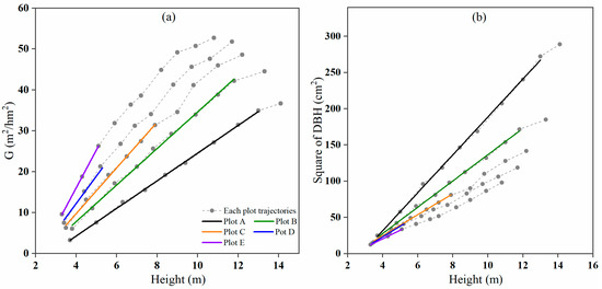
Figure 1.
The relationships between (a) basal area G and (b) square average diameter at breast height (D2) and H for plots A, B, C, D, and E.
For plot F (Figure 2a), the scatter plot of the stand basal area against average height showed three line segments. Line segment 1 demonstrated the relationship for mean heights from 5.3 m to 9.2 m, corresponding to the ages of 6 to 10 years. At this stage, the tree canopies changed from relatively open to closed, and natural pruning occurred but not self-thinning. The artificial thinning that was conducted at the ages of 10 and 11 years created space for the remaining trees to grow. Line segment 2 covered a longer period and was associated with the relationship between basal area and a mean height from 10.7 m to 15.2 m, corresponding to the ages of 12 to 22 years. Thinning at the ages of 10 and 11 years decreased the stand density and changed the slope of the basal area–mean height relationship, causing the slope of line segment 2 to differ from that of line segment 1. Line segment 3 revealed the relationship between basal area and stand mean height from 15.6 m to 16.5 m, corresponding to the ages of 24 to 30 years. At this stage, as the trees grew, the tree crowns and diameters became larger, and the stand development moved towards full stocking again, which slowed tree height growth and increased the slope of the basal area–mean height relationship. The corresponding linear relationships between and H are shown in Figure 2b.
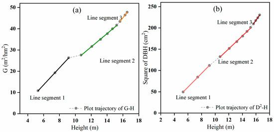
Figure 2.
The relationships between (a) basal area (G) and (b) square average diameter at breast height (D2) and H for plot F.
The relationships between G and H for plot A to F were modelled using a simple linear regression and are shown in Table 3. The estimated coefficients of the models were significantly different from zero at the significance level of 0.05, the R2 were greater than 0.995, and the RRMSE ranged from 0.07% to 10.44%. These results indicated that there was a significant linear relationship between G and H in the Chinese fir plantations. As the initial tree density increased, the absolute value of the intercept and the slope of the models increased.
Table 3.
The results of modelling the relationship between G and H for plots A to F (a and b are model coefficients; R2 is the coefficient of determination; RMSE is the root mean square error; RRMSE is the relative RMSE; and * indicates that the model parameter is significantly different from zero at a significance level of 0.05).
The relationship between G and H can be expressed as follows:
In the equation, the intercept and the slope vary depending on stand density. Given a fully stocked stand, both parameters can be considered constant. If b does not change, then the value of the derivative of is equivalent to zero. By incorporating Equation (6), it can be deduced that the derivative of is similarly equal to 0. Then, there is,
Based on Equation (7), it can be concluded that is equal to .
The following relationship was obtained:
where is the derivative of , which represents the annual increase in the stand basal area, and is the derivative of , which represents the annual increase in the average tree height. Equation (6) implies that for a stand with any stand density, as long as its growth of basal area and height meets Equation (8), its relative stand density does not change. This implies that a fully stocked stand can grow following Equation (8) until the relationship between basal area growth and height growth is broken, that is, when self-thinning occurs.
Based on the record of field observations and information in Table 2, the stand of plot F was fully stocked at the age of 10 years, but self-thinning had not yet taken place. The slope of the basal area–average height relationship from line segment 1 can be regarded as the exponent of the maximum size-density line. When the stand was fully stocked at the age of 10 years, and if artificial thinning was not conducted, then the trees in the stand would continue to grow for a certain period and then would start self-thinning. When fully stocked, the trees would grow by changing the ratio of height to D and become stable for some years. During this period, self-thinning might not necessarily occur. However, without artificial thinning, competition would become stronger and self-thinning would occur when the suppressed trees were not able to obtain enough light, water, and nutrients to grow.
With a slope of 4.0123, extending line segment 1 resulted in the potential maximum size-density line based on the relationship between stand basal area and average height for the fully stocked stand plot F. The extended line segment was used to define a stand growth balance status in which its stock density P1.0 = 1.0, the number of trees per hectare does not change, and the change rate in the basal area–average height relationship is zero. At the stage of the stand growth balance status, the annual growth rate of the basal area balanced the annual growth rate of the average height with a change rate of almost zero, meeting Equation (8). Because of the invariable number of trees, the annual growth rate of D also balanced the annual growth rate of the average height.
The aforementioned stand growth balance status was verified by the change in basal area and height growth rate over time, as shown in Table 4. During the period from 4 years to 6 years, Equation (8) was not met. However, at the ages of 8 and 10 years, the values of were very close to the values of . Significant differences occurred at the age of 12 years due to artificial thinning at the ages of 10 and 11 years. The similarity between the values of and was quickly achieved at the age of 14 years and was maintained until the stand was clear-cut at the age of 30 years.
Table 4.
The change in basal area and height growth rates over time for plot F.
The stand growth balance status was further verified by the observed trends in stand basal area and height growth rates over time from plots A, B, C, D, and E (Table 5). Plot A had similar growth rates of stand basal area and height from the age of 6 to 16 years. Self-thinning started to take place at the age of 16 years, which led to significantly different basal areas and height growth rates at the age of 18 years. Similar trends in basal area and height growth rates were found in plot B because self-thinning was very slight, although self-thinning started earlier than that in plot A. Plot C exhibited a significantly shorter duration of growth balance status than plots A and B, which can be attributed to its higher tree density. In plot C, the stand basal area and height growth rates were similar from the age of 6 to 10 years and became significantly different at the age of 12 years, at which time the self-thinning became stronger. In plots D and E, the period of growth balance status became much shorter due to higher tree densities and stronger and earlier tree competition. Self-thinning broke the growth balance status and led to slightly different and fluctuating growth rates of stand basal area and height.
Table 5.
The change in basal area and height growth rates over time for plots A to E.
3.2. The Trend in Stand G/H to the First Limit Value
Dividing both sides of Equation (6) by H and then calculating its first derivative results in:
Due to a negative value of the model intercept a, . Thus, the value increased in the stands due to a greater growth rate in the basal area than in the height before canopy closure and self-thinning (Figure 3). As the stands experienced canopy closure, however, the increase in the value slowed, and eventually, the value stabilized and approached a limit value. Once the value started to stabilize, self-thinning began. During the period of self-thinning, the stands grew, with the value remaining relatively constant (Figure 3a). Any artificial thinning could change this trend, but the stands would return with the value approaching its limit value (Figure 3b). The stands with different planting tree densities had different limit values and times for their values to approach the limit values. The higher the stand density is, the greater the limit values, the earlier the reaches the limit values, and the earlier the self-thinning starts. Theoretically, if , that is, , then, there is
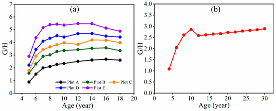
Figure 3.
The trend in G/H values over time for the fully stocked stands of (a) plots A, B, C, D, and E and (b) plot F.
Moreover, in Equations (6) and (8), because of a negative and constant intercept, as G increases, , then , and thus, , generally. That is, the basal area growth rate () should usually be larger than the height growth rate () in fully stocked stands. This is demonstrated in Figure 4, in which, overall, the growth rates of both stand basal area and average height decreased over time. However, the growth rates of the basal area were all greater than those of the average height for the stands with different planting tree densities of plots A, B, C, D, and E before canopy closure and self-thinning took place. As the stand canopies closed, the basal area growth was impeded due to limited space, and its growth rates decreased much faster than that of height, which led to the growth rate of the basal area becoming close to that of the average height for plots A, B, C, D, and E. Self-thinning might break the similarity and lead to fluctuations in both basal area and height growth rates, but both growth rates did not look very much different. The same trend was also noticed in the stand of plot F, but the artificial thinning that was conducted at the age of 10 and 11 years significantly changed the growth rate of the basal area. After just two years, the basal area growth rate returned to that of the height. The growth trends in the stand basal area and average height implied that the growths of the stand basal area and average height were allometric before canopy closure and self-thinning and became isogonic afterwards.
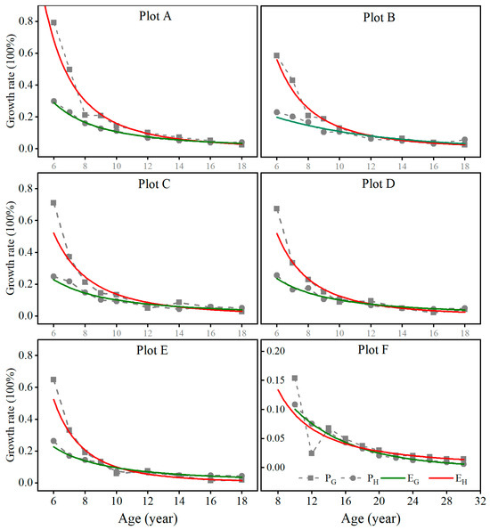
Figure 4.
The regression curve of growth rates of stand basal area and average height over time in the fully stocked stands with different planting tree densities. ( is the regression curve for the growth rates of stand basal area over time. is the regression curve for the growth rates of average height over time).
3.3. Trend in to the Second Limit Value
In Figure 5, for a given age, the H/D value increased from plot A to plots B, C, D, and E as the tree density increased. For a given tree density, the H/D value decreased from the age of 5 to 7 years and then continuously increased for plots A, B, C, D, and E. For plot F, the H/D value increased quickly before the age of 20 years and then slowly approached the second limit value.
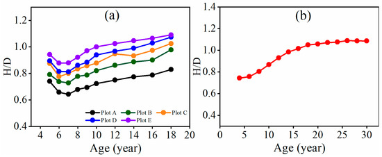
Figure 5.
The trend in H/D values over time for the fully stocked stands of (a) plots A, B, C, D, and E and (b) plot F.
In Figure 6, the growth rates of both average height and average DBH (simply called diameter) decreased over time. Moreover, for all the stands of plots A, B, C, D, and E, the growth rate of the average diameter was greater than that of the average height because space was sufficient for the expansion of tree crowns before the age of 7 years. Afterwards, the growth rate of the average height was consistently greater than that of the average diameter because the tree canopies started to close, and their diameter growth was impeded. However, the differences between the height and diameter rates became increasingly smaller. This indicated that the height and diameter growth in the stands was allometric even at the stage of canopy closure and self-thinning but showed an isogonic trend as the stand became mature. In the stand shown in Figure 6, plot F, the height growth rate was always greater than that of the diameter, but their difference consistently decreased and became similar to each other after 22 years of age, indicating a potential trend in isogonic growth after maturation.
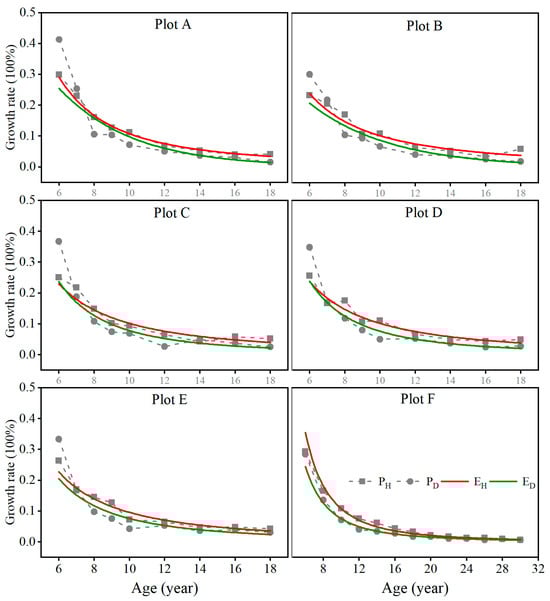
Figure 6.
The regression curve for the growth rates of stand average height and diameter over time in the fully stocked stands with different planting tree densities. ( is the regression curve for the growth rates of stand average height over time. is the regression curve for the growth rates of stand average diameter over time).
4. Discussion
The critical step for developing stand maximum size-density equations is the collection of data from fully stocked stands. Although substantial research has been conducted, there is still a lack of an operative and effective measure or indicator for identifying and selecting fully stocked stands [6,55,68,78]. In this study, we explored the growth characteristics of six fully stocked stands with five self-thinning stands and one artificial thinning stand and proposed the concept of growth balance status. We found that at the stage of growth balance status, the stands were fully stocked with an invariable slope for the relationship between stand basal area and average height, that is, was met and self-thinning had not occurred. Artificial thinning may break the growth balance status, but the change in stand density due to artificial thinning will adjust the growth of the basal area and height, which will make the stands eventually return to the growth balance status if the stands are young enough for growth.
Moreover, the time when the stands became fully stocked and entered the growth balance status varied depending on the planted tree densities. The higher the tree density, the earlier the time. Self-thinning will break the growth balance status and lead to fluctuating growth rates of the stand basal area and average height due to tree competition. Thus, the higher the tree density, the earlier self-thinning takes place and the shorter the time period of the growth balance status. However, the fluctuations in the growth rates of both basal area and average height due to self-thinning were slight and showed a trend in both growth rates becoming similar to each other, that is, PG ≈ PH. In addition, it was found that the G/H values of the stands increased before being fully stocked, became stable after canopy closure, and then approached their limit values at the self-thinning stage, implying similar basal area and height growth rates.
On the other hand, there have been substantial studies and debates on whether tree variables in fully stocked stands grow allometrically or isogonically [22,28,29,30,31]. In this study, we found that before canopy closure and self-thinning, the stand basal area growth rate was greater than the average height growth rate. As the stands became fully stocked and self-thinning took place, both the basal area and average height growth rates became similar to each other. This implied that the growth of the stand basal area and average height changed from allometric to isogonic. The average diameter growth rate was larger than the average height growth rate at the beginning and then decreased quickly and decreased more than the average height growth rate as the stands experienced canopy closure. This indicated that the growths of both the average height and diameter were allometric, and this was true even in the fully stocked and self-thinned stands. However, there was a trend in both the average height and diameter growth rates becoming similar as the stands matured.
The reason why the slopes of Reineke’s model and the −3/2nd power laws are different [21,29] can be explored using the theory of the two limit values. Because the second limit value is not reached at the canopy closure or self-thinning stages in many stands, the height growth rate is still larger than the diameter growth rate, and the growth relationship between height and diameter is allometric, not isogonic. The theory of the two limit values can also be applied to explore the reason why the self-thinning rates are different in different growth stages for one tree species. In fact, self-thinning in stands is determined by the relative growth relationship of height and diameter and is dynamic at different self-thinning stages. However, the initiation age of self-thinning cannot be determined accurately because the first limit value () is still difficult to obtain due to the lack of self-thinning data. However, the second limit value can be determined accurately because the height growth rate is equal to the diameter growth rate at this time. For stands with higher densities, the first limit value is reached earlier than the second limit value. If the limit extreme value is reached or will be reached, it can be speculated that the stand will begin to self-thin.
One of the arguments for self-thinning is that the self-thinning line can be straight or curved. Several studies have already demonstrated that the self-thinning line is curved because the actual slope of the self-thinning line becomes steeper with increasing age and tree size [5,81]. We speculate that there are two cases related to self-thinning: with and without dead trees removed promptly. Compared with the latter, the former will lead to an improvement in growing space and a reduction in competition, which will result in different self-thinning rates and trajectories. In our most recent study, we found that the self-thinning line was straight when dead trees were removed promptly; if dead trees were not removed, then the self-thinning line was curved. The latter situation is more prevalent in nature. However, it is still difficult to predict the curved self-thinning line accurately because the decomposition rate of dead trees varies with tree species and climate. Following this, an experimental study will be undertaken to examine the impacts of tree removal and non-removal on self-thinning trajectories.
The results of this study show that the growth balance status in which can provide a potential measure for identifying and selecting fully stocked stands before self-thinning, while the similar growth rates of stand basal area and average height, PG ≈ PH, offer an implication of fully stocked stands in which self-thinning is taking place. In practice, the existing stands can be first visually interpreted for their status of being fully stocked, stand basal area and average height and their growth rates can be measured and analysed to make a decision on whether the stands have been fully stocked, and then the data can be used to develop maximum size-density lines. For plantations, due to different site conditions and different numbers of trees planted, the time needed for stands to reach the growth balance status and the length of time for the stands to maintain the growth balance status may vary. However, the growth balance status does exist and can be used for the selection of fully stocked stands in which the growth rate of the per unit basal area is similar to that of the per unit average height.
5. Conclusions
In this study, the growth characteristics of stand variables from six fully stocked Chinese fir plantations with five self-thinned plots and one artificial thinned plot were investigated and analysed, which resulted in the following conclusions:
A highly significant linear relationship was observed between stand basal area and average height, with the absolute values of the intercepts and the slopes of the models increasing as the planted tree density increased.
After canopy closure and before self-thinning, there was a growth balance status of fully stocked stands in which , providing a potential measure that can be used to select fully stocked stands without self-thinning.
Before self-thinning, the growth rate of the stand basal area was greater than that of the average height. As the stands were fully stocked, the basal area growth rate decreased quickly and became similar to the average height growth rate at the self-thinning stage. The isogonic growth of basal area and average height can be utilised as an indicator for the selection of fully stocked and self-thinned stands.
As the stands experienced canopy closure, the value became stable and approached the first limit value. The stands with different planting tree densities had different limit values. Meanwhile, the H/D value may approach the second limit value after the stands become mature. The two limit values may be reached at the same time given suitable stand density, and this density may be appropriate for plantation management.
The growths of average diameter and height were allometric before the stands became mature and then showed an isogonic trend.
Author Contributions
Conceptualization, S.L. and S.Z.; methodology, S.L.; software, H.X.; validation, S.Z., H.X. and Z.G.; formal analysis, S.Y.; investigation, Z.G.; resources, S.Z.; data curation, S.Y.; writing—original draft preparation, S.L.; writing—review and editing, S.Z.; visualization, H.X.; supervision, S.Z.; project administration, S.Z.; funding acquisition, S.Z. All authors have read and agreed to the published version of the manuscript.
Funding
This study was financially supported by the Forestry Public Welfare Scientific Research Project of China, funding number 201504301.
Data Availability Statement
The data that support the findings of this study are available on request from the corresponding author, upon reasonable request.
Conflicts of Interest
The authors declare no conflict of interest.
References
- Zhang, J.; Oliver, W.W.; Powers, R.F. Reevaluating the self-thinning boundary line for ponderosa pine (Pinus ponderosa) forests. Can. J. For. Res. 2013, 43, 963–971. [Google Scholar] [CrossRef]
- De Prado, D.R.; Martín, R.S.; Bravo, F.; de Aza, C.H. Potential climatic influence on maximum stand carrying capacity for 15 Mediterranean coniferous and broadleaf species. For. Ecol. Manag. 2020, 460, 117824. [Google Scholar] [CrossRef]
- Jack, S.B.; Long, J.N. Linkages between silviculture and ecology: An analysis of density management diagrams. For. Ecol. Manag. 1996, 86, 205–220. [Google Scholar] [CrossRef]
- Lei, X.D.; Tang, S.Z.; Fu, L.Y. Quantitative Evaluation of Forest Site Quality—Theory, Method and Application; Chinese Forestry Press: Beijing, China, 2019. [Google Scholar]
- Zeide, B. How to measure stand density. Trees 2005, 19, 1–14. [Google Scholar] [CrossRef]
- Burkhart, H.E. Comparison of maximum size-density relationships based on alternate stand attributes for predicting tree numbers and stand growth. For. Ecol. Manag. 2013, 289, 404–408. [Google Scholar] [CrossRef]
- Reineke, L.H. Perfecting a stand-density index for even-aged forests. J. Agric. Res. 1933, 46, 627–638. [Google Scholar]
- Yang, Y.; Titus, S.J. Maximum size-density relationship for constraining individual tree mortality functions. For. Ecol. Manag. 2002, 168, 259–273. [Google Scholar] [CrossRef]
- Vospernik, S.; Sterba, H. Do competition-density rule and self-thinning rule agree? Ann. For. Sci. 2015, 72, 379–390. [Google Scholar] [CrossRef]
- Burkhart, H.E.; Tomé, M. Modelling Forest Trees and Stands; Springer: Dordrecht, The Netherlands, 2012. [Google Scholar]
- Yoda, K.; Kira, T.; Ogawa, H.; Hozumi, K. Self-thinning in overcrowded pure stand under cultivated and natural conditions. J. Biol. Osaka City Univ. 1963, 14, 107–129. [Google Scholar]
- White, J.; Harper, J.L. Correlated changes in plant size and number in plant populations. J. Ecol. 1970, 58, 467–485. [Google Scholar] [CrossRef]
- West, G.B.; Brown, J.H.; Enquist, B.J. A general model for the origin of allometric scaling laws in biology. Science 1997, 276, 122–126. [Google Scholar] [CrossRef]
- West, G.B.; Brown, J.H.; Enquist, B.J. A general model for the structure and allometry of plant vascular systems. Nature 1999, 400, 664–667. [Google Scholar] [CrossRef]
- Gorham, E. Shoot height, weight and standing crop in relation to density of monospecific plant stands. Nature 1979, 279, 148–150. [Google Scholar] [CrossRef]
- White, J. Demographic Factors in Populations of Plants; University of California Press: Berkeley, CA, USA, 1980. [Google Scholar]
- White, J. The allometric interpretation of self-thinning rule. J. Theor. Biol. 1981, 89, 475–500. [Google Scholar] [CrossRef]
- Cousens, R.; Hutchings, M.J. The relationship between density and mean frond weight in monospecific seaweed stands. Nature 1983, 301, 240–241. [Google Scholar] [CrossRef]
- Charru, M.; Seynave, I.; Morneau, F.; Rivoire, M.; Bontemps, J.D. Significant differences and curvilinearity in the self-thinning relationships of 11 temperate tree species assessed from forest inventory data. Ann. For. Sci. 2012, 69, 195–205. [Google Scholar]
- Weller, D.E. A reevaluation of the—3/2 power rule of plant self-thinning. Ecol. Monogr. 1987, 57, 23–43. [Google Scholar] [CrossRef]
- Weller, D.E. Self-thinning exponent correlated with allometric measures of plant geometry. Ecology 1987, 68, 813–821. [Google Scholar] [CrossRef]
- Fang, J.Y. Self-thinning rule in plant population. Rural Eco-Environ. 1992, 2, 7–12, (In Chinese with English Abstract). [Google Scholar]
- Li, F.R. A review on stand density-about the 3/2 Power Law. For. Res. 1995, 8, 25–32, (In Chinese with English Abstract). [Google Scholar]
- Osawa, A. Inverse relationship of crown fractal dimension to self-thinning exponent of tree population: A hypothesis. Can. J. For. Res. 1995, 25, 1608–1617. [Google Scholar] [CrossRef]
- Kikuzawa, K. Theoretical relationships between mean plant size, size distribution and self-thinning under one-sided competition. Ann. Bot. 1999, 83, 11–18. [Google Scholar] [CrossRef][Green Version]
- Wu, C.Z.; Hong, W. A study on the self-thinning law of Chinese fir plantation. Sci. Silvae Sin. 2000, 36, 97–101, (In Chinese with English Abstract). [Google Scholar]
- Del Río, M.; Montero, G.; Bravo, F. Analysis of diameter-density relationships and self-thinning in non-thinned even-aged Scots pine stands. For. Ecol. Manag. 2001, 142, 79–87. [Google Scholar] [CrossRef]
- Luis, J.F.S.; Fonseca, T.F. The allometric model in the stand density management of Pinus pinaster Ait. Ann. For. Sci. 2004, 61, 807–814. [Google Scholar] [CrossRef]
- Pretzsch, H.; Biber, P. A reevaluation of Reineke’s rule and stand density index. For. Sci. 2005, 51, 304–320. [Google Scholar]
- Vanclay, J.K.; Sands, P.J. Calibrating the self-thinning frontier. For. Ecol. Manag. 2009, 259, 81–85. [Google Scholar] [CrossRef]
- Rivoire, M.; Moguedee, G.L. A generalized self-thinning relationship for multi-species and mixed-size forests. Ann. For. Sci. 2012, 69, 207–219. [Google Scholar] [CrossRef]
- Mohler, C.L.; Marks, P.L.; Sprugel, D.G. Stand structure and allometry of tree during self-thinning of pure stand. J. Ecol. 1978, 68, 598–614. [Google Scholar]
- Ogawa, K. Time-trajectory of mean phytomass and density during a course of self-thinning in a sugi (Cryptomeria japonica D. Don) plantation. For. Ecol. Manag. 2005, 214, 104–110. [Google Scholar] [CrossRef]
- Aguirre, A.; del Rio, M.; Condes, S. Intra- and inter-specific variation of the maximum size-density relationship along an aridity gradient in Iberian pinewoods. For. Ecol. Manag. 2018, 411, 90–100. [Google Scholar] [CrossRef]
- Andrews, C.; Weiskittel, A.; D’Amato, A.W.; Simons-Legaard, E. Variation in the maximum stand density index and its linkage to climate in mixed species forests of the North American Acadian Region. For. Ecol. Manag. 2018, 417, 90–102. [Google Scholar] [CrossRef]
- Zeide, B. Tolerance and self-tolerance of trees. For. Ecol. Manag. 1985, 13, 149–166. [Google Scholar] [CrossRef]
- Yang, S.; Burkhart, H.E. Estimation of carrying capacity in loblolly pine (Pinus taeda L.). For. Ecol. Manag. 2017, 385, 167–176. [Google Scholar] [CrossRef]
- Zeide, B. Analysis of the—3/2 power rule of plant self-thinning. For. Sci. 1987, 33, 517–537. [Google Scholar]
- Sackville Hamilton, N.R.; Matthew, C.; Lemaire, G. In defence of the—3/2 boundary rule: A re-evaluation of self-thinning concepts and status. Ann. Bot. 1995, 76, 569–577. [Google Scholar] [CrossRef]
- Zhang, L.J.; Bi, H.Q.; Jeffrey, H.G.; Linda, S.H. A comparison of alternative methods for estimating the self-thinning boundary line. Can. J. For. Res. 2005, 35, 1507–1514. [Google Scholar] [CrossRef]
- Possato, E.L.; Calegario, N.; Nogueira, G.S.; Melo, E.D.; Alves, J.D. Estimate of stand density index for Eucalyptus urophylla using different fit methods. Rev. Arvore 2016, 40, 921–929. [Google Scholar] [CrossRef]
- Trouvé, R.; Nitschke, C.R.; Robinson, A.P.; Baker, P.J. Estimating the self-thinning line from mortality data. For. Ecol. Manag. 2017, 402, 122–134. [Google Scholar] [CrossRef]
- Meng, J.H. A comparison of different methods for fitting the self-thinning equation. J. Beijing For. Univ. 2019, 41, 58–68, (In Chinese with English Abstract). [Google Scholar]
- Westoby, M. The self-thinning rule. Adv. Ecol. Res. 1984, 14, 167–225. [Google Scholar]
- Wilson, F.G. Thinning as an orderly discipline: A graphic spacing schedule for red pine. J. For. 1979, 77, 483–486. [Google Scholar]
- Sterba, H. Estimating potential density from thinning experiments and inventory data. For. Sci. 1987, 33, 1022–1034. [Google Scholar]
- Zeide, B. Self-thinning and stand density. For. Sci. 1991, 37, 517–523. [Google Scholar]
- Zeide, B. A relationship between size of trees and their number. For. Ecol. Manag. 1995, 72, 265–272. [Google Scholar] [CrossRef]
- Zeide, B. Natural thinning and environmental change: An ecological process model. For. Ecol. Manag. 2001, 154, 165–177. [Google Scholar] [CrossRef]
- Zeide, B. Analysis of a concept: Stand density. J. Sustain. For. 2002, 14, 51–62. [Google Scholar] [CrossRef]
- Zeide, B. Comparison of self-thinning models: An exercise in reasoning. Trees 2010, 24, 1117–1126. [Google Scholar] [CrossRef]
- Lynch, T.B.; Wittwer, R.F.; Stevenson, D.J.; Huebschmann, M.M. A maximum size-density relationship between Lorey’s mean height and trees per hectare. For. Sci. 2007, 53, 478–485. [Google Scholar]
- Inoue, A.; Nishizono, T. Allometric model of the Reineke equation for Japanese cypress (Chamaecyparis obtuse) and red pine (Pinus densiflora) stands. J. For. Res. 2004, 9, 319–324. [Google Scholar] [CrossRef]
- Woodall, C.W.; Miles, P.D.; Vissage, J.S. Determining maximum stand density index in mixed species stands for strategic-scale stocking assessments. For. Ecol. Manag. 2005, 216, 367–377. [Google Scholar] [CrossRef]
- Ducey, M.J.; Knapp, R.A. A stand density index for complex mixed species forests in the northeastern United States. For. Ecol. Manag. 2010, 260, 1613–1622. [Google Scholar] [CrossRef]
- Miyanishi, K.; Hoy, A.R.; Cavers, P.B. Generalized law of self-thinning in plant-populations. J. Theor. Biol. 1979, 78, 439–442. [Google Scholar] [CrossRef]
- Weiner, J.; Thomas, S.C. Size variability and competition in plant monocultures. Oikos 1986, 47, 211–222. [Google Scholar] [CrossRef]
- Forrester, D.I. Linking forest growth with stand structure: Tree size inequality, tree growth or resource partitioning and the asymmetry of competition. For. Ecol. Manag. 2019, 447, 139–157. [Google Scholar] [CrossRef]
- Lee, D.; Choi, J. Evaluating maximum stand density and size-density relationships based on the competition density rule in Korean pines and Japanese larch. For. Ecol. Manag. 2019, 446, 204–213. [Google Scholar] [CrossRef]
- Ge, F.W.; Zeng, W.; Ma, W.; Meng, J. Does the slope of the self-thinning line remain a constant value across different site qualities? An Implication for Plantation Density Management. Forests 2017, 8, 355. [Google Scholar] [CrossRef]
- Fu, L.H.; Zhang, J.G.; Duan, A.G.; Sun, H.G.; He, A.Y. Review of studies on maximum size-density rule. J. Plant Ecol. 2008, 32, 501–511, (In Chinese with English Abstract). [Google Scholar]
- Cheng, Z.C.; Chen, L.; Wang, G.; Zeng, S.; Fang, S. Models of Management Planning System for Pinus massoniana Forests; Chinese Forestry Press: Beijing, China, 1991. [Google Scholar]
- Cheng, Z.C.; Zeng, S. Study on Silvicultural Types and Growth and Yield Tables for Water Conservation Forests of Pinus massoniana; Chinese Forestry Press: Beijing, China, 2003. [Google Scholar]
- Fang, H.L. Evaluation of stand density index for 894 existing forests. J. Northeast For. Univ. 1995, 23, 100–105, (In Chinese with English Abstract). [Google Scholar]
- Wang, D.S. Study on stand density. For. Resour. Manag. 1994, 1, 67–71, (In Chinese with English Abstract). [Google Scholar]
- Liu, J.F.; Tong, S.Z. Growth process table of Chinese fir plantation. For. Res. 1995, 8, 164–169, (In Chinese with English Abstract). [Google Scholar]
- Liu, J.F.; Jiang, X.; Hong, W. Variable stand density yield prediction table of Pinus massoniana Lamb. Plantation in Fujian. J. Jilin For. Univ. 1999, 14, 206–209, (In Chinese with English Abstract). [Google Scholar]
- Luo, Q.B.; Zeng, W.S.; He, D.B. Model, Theory, Method and Application of Forestry Tables; Hunan Science and Technology Press: Changsha, China, 2001. [Google Scholar]
- Meng, X.Y. Forest Measurement; Chinese Forestry Press: Beijing, China, 2006. [Google Scholar]
- Che, S.H.; Zhang, J.G. Study on stand density index of Chinese fir plantation based on self-thinning rule. Bull. Bot. Res. 2012, 32, 343–347. [Google Scholar]
- Zhang, H.R. Research Method and Practice in Forest Management; Chinese Forestry Press: Beijing, China, 2018. [Google Scholar]
- Fang, J.Y.; Kan, M.; Yamakura, T. Relationships between population growth and population density in monocultures of Larix Leptolepis. Acta Bot. Sin. 1991, 33, 949–995, (In Chinese with English Abstract). [Google Scholar]
- Bi, H.Q.; Turvey, N.D. A method of selecting data points for fitting the maximum biomass- density line for stands undergoing self- thinning. Aust. Ecol. 1997, 22, 356–359. [Google Scholar] [CrossRef]
- Newton, P.E. Asymptotic size-density relationships within self-thinning black spruce and jack pine stand-types: Parameter estimation and model reformulations. For. Ecol. Manag. 2006, 226, 49–59. [Google Scholar] [CrossRef]
- Xue, L.; Ogawa, K.; Hagihara, A.; Liang, S.; Bai, J. Self-thinning exponents based on the allometric model in Chinese pine (Pinus tabulaeformis Carr.) and Prince Rupprecht’s larch (Larix principis-rupprechtii Mayr) stands. For. Ecol. Manag. 1999, 117, 87–93. [Google Scholar] [CrossRef]
- Solomon, D.S.; Zhang, L.J. Maximum size-density relationships for mixed softwoods in the northeastern USA. For. Ecol. Manag. 2002, 155, 163–170. [Google Scholar] [CrossRef]
- Huang, C.Z. stand basal area-volume tables of Schima superba Gardn. Et Champ. Plantation in Eastern Fujian. J. Fujian For. Sci. Technol. 2011, 38, 54–57, (In Chinese with English Abstract). [Google Scholar]
- VanderSchaaf, C.L. Estimating individual stand size-density trajectories and a maximum size-density relationship species boundary line slope. For. Sci. 2010, 56, 327–335. [Google Scholar]
- Xue, L.; Hagihara, A. Summary and evaluation of the researches on the self-thinning pure stands. Acta Ecol. Sin. 2001, 21, 835–838, (In Chinese with English Abstract). [Google Scholar]
- Tong, S.Z.; Sheng, W.T.; Zhang, J.G. Studies on the density effects of Chinese fir stands. For. Res. 2002, 15, 66–75, (In Chinese with English Abstract). [Google Scholar]
- Meyer, W.H. Yield of even-aged stands of ponderosa pine. USDA Tech. Bull. 1938, 630, 59. [Google Scholar]


Disclaimer/Publisher’s Note: The statements, opinions and data contained in all publications are solely those of the individual author(s) and contributor(s) and not of MDPI and/or the editor(s). MDPI and/or the editor(s) disclaim responsibility for any injury to people or property resulting from any ideas, methods, instructions or products referred to in the content. |
© 2023 by the authors. Licensee MDPI, Basel, Switzerland. This article is an open access article distributed under the terms and conditions of the Creative Commons Attribution (CC BY) license (https://creativecommons.org/licenses/by/4.0/).