Multistage Sampling and Optimization for Forest Volume Inventory Based on Spatial Autocorrelation Analysis

Abstract

It is important to achieve estimates at the minimum cost, with no greater uncertainty than that which is appropriate for the objectives of the inventory. The aim of this study was to estimate the forest volume efficiently and accurately by sampling and analyzing the existing forest survey data, which is also a technical challenge. In this work, we used the spatial statistics tools in the ArcGIS software to analyze spatial autocorrelations with the data from the sixth to ninth continuous forest inventories (CFI) of Sichuan Province from 2002, 2007, 2012, and 2017. Based on the sampling framework of the CFI, we divided the sampling units into five groups using different methods to create the second-stage samples. Combined with the spatial autocorrelation analysis results, we selected certain samples from the collection of second-stage samples through stratified sampling to form the third-stage sampling units. We applied the sampling ratio, sampling accuracy, workload, and costs as the evaluation indexes for the sampling efficiency analysis. The main results are as follows: Before conversion, the forest volume density had a positively skewed distribution. There was substantial positive spatial autocorrelation, and its intensity was affected by the distance scale, especially at 187.3 km, where the spatial processes of clustering were most pronounced. At the significance level of α = 0.01, the high-volume stands were mainly concentrated in the Aba Prefecture, Garze Prefecture, and Liangshan Prefecture, while the low-volume stands were mainly concentrated in the Sichuan Basin region. The heterogeneous gatherings were staggered between the high-volume areas and low-volume areas, while the transition zone between the three prefecture regions and basin region was randomly distributed. With 95% reliability, the average estimation accuracy of the systematic sampling, random sampling, and cluster sampling in the second stage was 94.09%, which is less accurate than the CFI estimation accuracy. The mean correlation coefficients (R) between the estimated value of the forest volume and the observations of the systematic sampling, random sampling, and cluster sampling in the second stage were 0.95, 0.98, and 0.96, respectively. The relative differences (RD%) were −0.52, −0.39, and −0.36, respectively. The spatial stratified sampling in the third stage, which is based on spatial distribution pattern information, significantly reduced the sampling ratio to 1.68 per 10,000, compared with the average ratios of the CFI sampling and second-stage sampling, which were 13.73 per 10,000 and 2.75 per 10,000, respectively. With 95% reliability, the mean accuracy of the spatial stratified sampling in the third stage was 93.05%, the R was 0.94, and the RD% was −0.09. Spatial stratified sampling is more in line with the actual work conducted in annual surveys because it effectively reduces the sample size using prior spatial information, which can better meet the requirements of the annual output.

1. Introduction

The efficient and accurate monitoring of the forest volume and its dynamic change is a popular topic of research in the field of natural resource investigation and monitoring [1,2,3], which also constitutes a technical challenge [4]. It is important to achieve the estimates at the minimum cost with no more uncertainty than that which is appropriate for the objectives of the inventory. Information required for decision making is acquired by using inventories to estimate the means and total measures of the forest characteristics, including the volume of the growing stock, which is the principal commercial product of forests, within a defined area. Due to the cost limitation of the field survey, it is impossible to measure every tree in order to investigate the forest volume because of the large areas involved. Therefore, the acquisition of information is typically based on sampling. Simple random sampling is the easiest technique through which a sample can be selected, but it is certainly not the only one. Significantly, there are other sampling techniques that have the great advantage of potentially leading to a reduction in the size of the confidence limit of the given parameter that is being estimated for a population. Analyses of the existing forest survey data can improve the sampling efficiency and estimation accuracy [5,6,7]. Research on sampling techniques focused on the acquisition of auxiliary data by remote sensing, applied using various approaches. Due to the requirements of accuracy and reliability, reducing the sampling units by improving the sampling methods and applying historical data is a key scientific problem [8]. With the implementation of a series of forestry policies to promote the construction of an ecological civilization and to address global climate change, the need for annual indicators of forest volumes is particularly urgent [9].

There are several feasible approaches to the production of annual estimates of forest volumes using CFI data [10]. The most straightforward approach simply uses the panel data to obtain estimates for the current year to reflect the current conditions. A drawback to this approach is that its inferential precision may be unacceptable. The second approach is joint estimation following the uniform grouping of the plots [2,11]. The precision of this approach is increased because the data for all the sample plots are used for the estimation. A third approach is to update the initial estimates obtained from an estimator, which can be design- or model-based, for the current year [1]. The optimization of the sampling system, which aims to improve the efficiency in order to reduce the workload that is currently in effect in forest resource investigation and monitoring, is necessary [2,3]. Sampling methods and techniques are key to obtaining forest resource information. Researchers widely used equiprobability sampling, which is the classic method [12,13]. Unequal probability sampling, spatial sampling, and adaptive sampling are more targeted toward forest volume inventories when the forest is not randomly distributed [14]. The merging and optimization of various sampling methods and techniques to improve the inventory efficiency based on the general applications and targeted supplements in the field of forest ecosystem dynamic monitoring became a developing trend [15,16]. The sampling methods used in national-scale forest resource surveys and monitoring in the United States, Canada, Germany, and Switzerland include stratified sampling, three-stage sampling, and stratified double sampling, which have their own advantages and disadvantages [17,18]. Research investigating sampling techniques focused on producing unbiased annual estimates for the forest inventory and data analysis, applying various approaches [19].

Spatial sampling is based on geostatistics known as geological statistics [20,21,22], which are also widely used in ecological research [23]. In forestry, geostatistics improve the precision and reliability of the estimation because they enable the segregation of different forest sites and ensure the representativeness of the estimations while improving the precision of the estimates and enabling a decreased sampling intensity [24,25]. An ecosystem is a dynamic equilibrium system with high spatial and temporal heterogeneity that is composed of a biotic community and its living environment. The difference between the spatial sampling technique and classical sampling technique lies in the consideration of the spatial autocorrelation of the research objects, possessing a wide range of applications in the field of natural resource surveying and monitoring [26]. Geostatistical interpolation proved to be a useful tool for studying spatial variation in forest carbon density [27]. We used geostatistics to guide the development of a sampling strategy that can reduce the number of plots to be measured while maintaining a high degree of accuracy and precision.

Angle count sampling was introduced in 1957 as an improvement on the ocular estimation technique, and stratified sampling was first attempted in 1963 in China. Since then, the forest inventory technique progressively transitioned from ocular estimation to statistical sampling. Meanwhile, research and experimentation focused on inventory methods that are suitable for different areas, conditions, and management levels, such as two-stage and multistage sampling inventories, double sampling with regression, and regression-based surveys combined with visual estimation and field mensuration, etc. Most of these methods were already put into practice [9]. In 2021, The National Forestry and Grassland Administration organized the comprehensive ecological monitoring of forests and grasslands on the national scale. Based on this continuous forest inventory sampling, one-fifth of the plots are investigated every year, and four-fifths of the samples are updated by remote sensing interpretation and modeling. Then, the forest volume is estimated in all the provinces of China according to the “1/5 + 4/5” joint estimation approach [2]. This comprehensive national ecological monitoring of forests and grassland optimized the survey organization process. The sampling method still employs an equal probability sampling technique. The number of sample units to be investigated by equiprobability sampling still accounts for approximately 20% of all the plots according to the specified accuracy and reliability. The systematic sampling method can reduce the sampling efficiency when there is substantial spatial autocorrelation in the distribution of the forest resources [28,29,30]. Systematic sampling reduces the correlation between plots. When the forest resources are distributed in clusters, the estimation accuracy may not meet the requirements, which increases the uncertainty regarding the sources of error [31,32]. Optimizing the sampling design and estimation methods to reduce the survey samples is a key problem in the monitoring of forest resources. In this study, we analyzed the characteristics of the timeseries and spatial distribution patterns of the forest volume by spatial autocorrelation. We optimized the multistage unequal probability sampling design for the annual monitoring of the forest volume based on the results of the timeseries and spatial distribution analyses. We updated the data according to the established growth model. Here, we demonstrate that a set of spatial unequal probability sampling techniques and methods should be formed in line with the annual monitoring of the forest volume to improve the inventory efficiency and, thus, to ensure the timely, accurate, and rapid acquisition of the forest volume information.

2. Research Area and Data Sources

2.1. Research Area

Sichuan Province is located in the hinterland of Southwest China, straddling five geomorphic units: the Sichuan Basin, Qinghai–Tibet Plateau, Hengduan Mountains, Yunnan–Guizhou Plateau, and Qinba Mountains. The province is a transition zone between the eastern monsoon region and the Qinghai–Tibet Plateau in Southwest China, and it is the second-largest forest region and fifth-largest pastoral region in China. The forest resources are primarily natural stands, which are mainly distributed throughout the western plateau and pelvic mountains. The region is one of the thirty-four biodiversity hotspots in the world. The main forest types include Abies Fabri, Picea asperata, Tsuga Chinensis, Larix Potaninii, Pinus tabulaeformis, Pinus armandii, Pinus Massoniana, Pinus Yunnanensis, Pinus densata, Cunninghamia Lanceolata, Cupressus funebris, Quercus, Betula, and Populus, as well as various mixed stands. According to the data of the ninth National Forest Resources Inventory [33], the forest area of Sichuan Province is 18.3977 million hectares (ha), and the forest coverage rate is 38.03%. The volume of arboreal species is 1.9720 billion m³, and the forest volume is 1.8610 billion m³.

2.2. Data Sources

We obtained the data used in this paper from the sixth (2002), seventh (2007), eighth (2012), and ninth (2017) continuous forest inventories (established in 1979) of Sichuan Province. Taking the entire province as a whole, we adopted the systematic sampling theory to arrange the plots in alternating intervals of 4 km × 8 km and 8 km × 8 km, with the plots successively crossing each other. We established a total of 10,098 permanent plots, as shown in Figure 1. The side length of the square plot was 25.82 m, and the area was 0.0667 ha. We measured the species, size, relative location, and other characteristics of each tree in the plots. The diameter of the smallest tree was 5 cm [34].

3. Methods

3.1. Forest Volume Calculation

We calculated the stand volume of the trees using volume models, with the diameter at breast height as the independent variable [35]. We obtained the volume of the sample plot after the summation. The unit of the forest volume is the cubic meter (m³).

3.2. Spatial Autocorrelation Analysis

The spatial autocorrelation of the forest volume was studied using geostatistics combined with the Moran index, employing the spatial statistics tools in ArcGIS10.2 software by Esri.

3.2.1. Global Spatial Autocorrelation

We measured the spatial autocorrelation based on the feature locations and attribute values using global Moran index statistics. The formula for global spatial autocorrelation analysis is as follows:

$$I=\left(\frac{n}{{\displaystyle \sum _{i=1}^n{\displaystyle \sum _{j=1}^n{w}_{ij}}}}\right)\cdot \frac{{\displaystyle \sum _{i=1}^n{\displaystyle \sum _{j=1}^n{w}_{ij}}(x_i-\overline{x})(x_j-\overline{x})}}{{\displaystyle \sum _{i=1}^n{(x_i-\overline{x})}^2}}$$

(1)

where I is the global Moran index; n is the number of sample plots; x_i and x_j are the stand volume values of positions i and j, respectively; $\overline{x}$ is the average stand volume value of all the sample plots; and w_ij is the spatial weight matrix values.

The z-score value is calculated as follows:

$$z-score=\frac{I-E(I)}{\sqrt{Var(I)}}$$

(2)

where E(I) is the expectation value, and Var(I) is the variance.

3.2.2. Incremental Spatial Autocorrelation

We used the incremental spatial autocorrelation tool to calculate the greatest distance in the spatial clustering pattern, which we used as the scale parameter for the local spatial autocorrelation analysis. This tool measures the spatial autocorrelation for a series of distances, with the option of creating a line graph of those distances and their corresponding z-scores. The z-scores reflect the intensity of the spatial clustering, and statistically significant peak z-scores indicate distances in which the spatial processes promoting clustering are most pronounced.

3.2.3. Local Spatial Autocorrelation

Using a set of weighted features, we can identify statistically significant hot spots, cold spots, and spatial outliers using the local Moran index statistics. The local Moran index formula is as follows:

$$I_i=\left(\frac{n^2}{{\displaystyle \sum _i^n{\displaystyle \sum _j^n{w}_{ij}}}}\right)\cdot \frac{(x_i-\overline{x}){\displaystyle \sum _j^n{w}_{ij}}(x_j-\overline{x})}{{\displaystyle \sum _i^n{(x_i-\overline{x})}^2}}$$

(3)

where I_i is the local Moran index; n is the number of sample plots; x_i and x_j are the stand volume values of positions i and j, respectively; $\overline{x}$ is the average stand volume value of all the sample plots; and w_ij is the spatial weight matrix values.

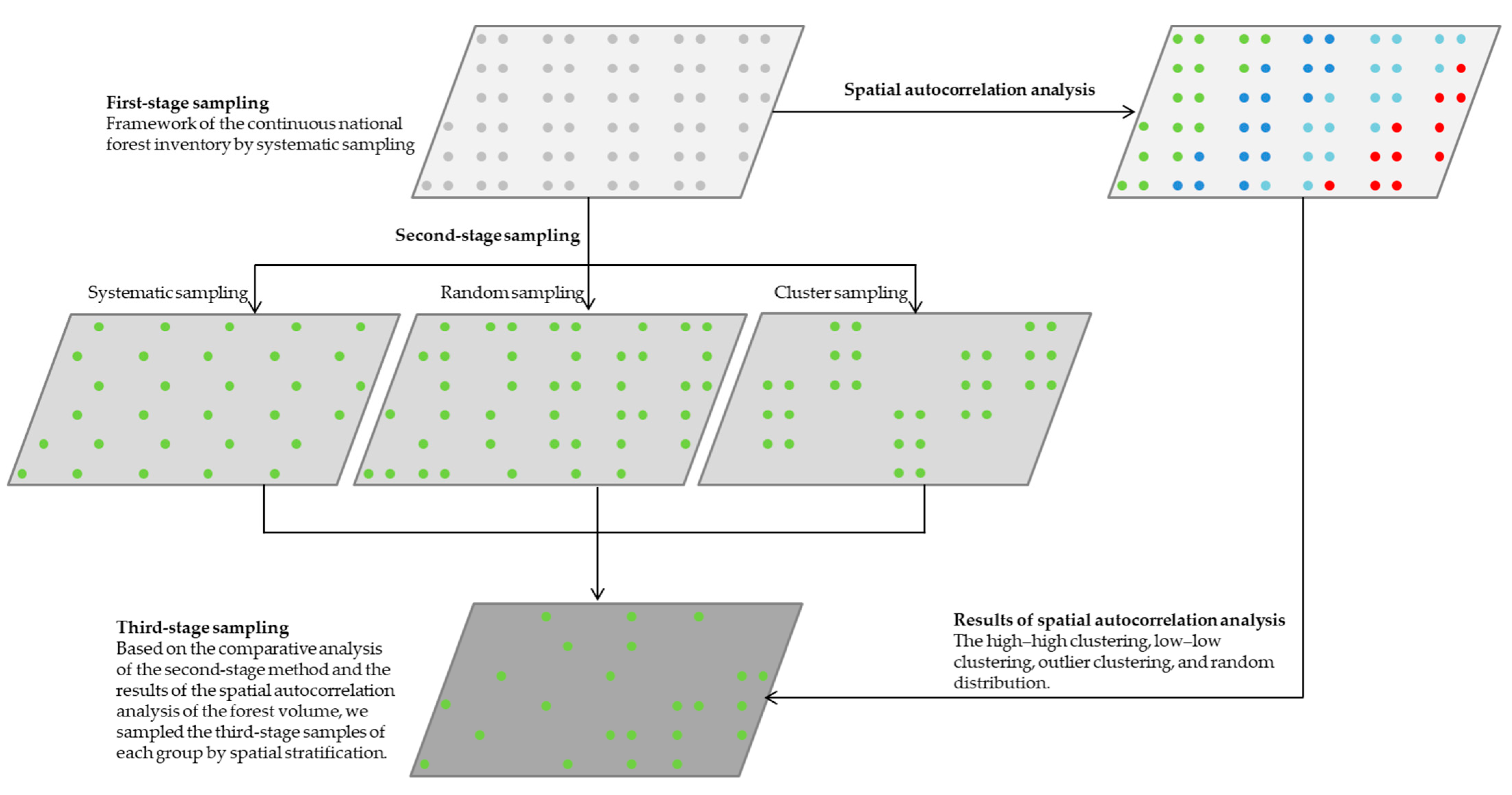
3.3. Sampling Design

3.3.1. The Multistage Sampling Frame

Based on the sampling framework of the continuous national forest inventory, we evenly divided the sampling units into five groups to form the second-stage sample units. The systematic sampling plots, random sampling plots, and cluster sampling plots were sampled according to the fixed spatial intervals, the random numbers, and the principle of minimum variation between counties, respectively. We compared different methods of sampling in the second stage for the third-stage sampling, and then we performed the third-stage spatial stratified sampling using the forest volume spatial autocorrelation results, as shown in Figure 2.

3.3.2. Second-Stage Sampling Methods

We organized the second-stage sampling units by systematic sampling, random sampling, and cluster sampling based on the sampling framework of the continuous national forest inventory.

3.3.3. Third-Stage Spatial Sampling

In design-based sampling, the population of values in a region is considered to be fixed, and randomness is introduced through the process of selecting the locations to be sampled. The research area is divided into several regions. The total sample size is calculated according to the method of the stratified sampling model, and then, the sample size is allocated to each region according to the weight of the spatial stratified sampling. Based on the comparative analysis of the second-stage method and the results of the spatial autocorrelation analysis of the forest volume, we sampled the third-stage samples of each group by spatial stratification.

3.4. Method of Estimation

For the population mean of the h layer, we performed a simple estimation through the stratified random sampling of the survey samples and auxiliary samples of each layer before the joint estimation. The mean and variance in the joint ratio estimation are as follows:

$${\overline{y}}_{RU}={\widehat{R}}_U\cdot \overline{X}=\frac{{\overline{y}}_{st}}{{\overline{x}}_{st}}\cdot \overline{X}=\frac{{\displaystyle \sum _{h=1}^L{W}_h{\overline{y}}_h}}{{\displaystyle \sum _{h=1}^L{W}_h{\overline{x}}_h}}\cdot \overline{X}$$

(4)

$$V({\overline{y}}_{RU})\approx {\displaystyle \sum _h^L{W}_h^2\frac{(1-f_h)}{n_h}(s_{yh}^2+{\widehat{R}}_U^2{s}_{xh}^2-2{\widehat{R}}_U{r}_h{s}_{yh}{s}_{xh})}$$

(5)

where ${\overline{y}}_{RU}$ is the population mean of the joint ratio estimation; $V({\overline{y}}_{RU})$ is the variance in the joint ratio estimation; ${\widehat{R}}_U$ is the ratio; $\overline{X}$ is the mean value of the observations; and $W_h$ is the weight of each layer. Here, we present the mean and variance in the joint regression estimation in Equations (6) and (7), respectively:

$${\overline{y}}_{lU}={\overline{y}}_{st}+{\alpha }_h(\overline{X}-{\overline{x}}_{st}).$$

(6)

When ${\alpha }_h$ is the predefined value of the h layer, the variance in the joint regression estimator is as follows:

$$V({\overline{y}}_{lU})\approx {\displaystyle \sum _h^L{W}_h^2\frac{(1-f_h)}{n_h}}(s_{yh}^2+{\alpha }^2{s}_{xh}^2-2\alpha s_{yxh}).$$

(7)

When ${\alpha }_h$ is the slope of the linear regression of the h-layer samples, the joint regression estimation is biased, but it meets the requirement of asymptotic consistency, and the variance in the hierarchical regression estimator is as follows:

$$V({\overline{y}}_{lU})={\displaystyle \sum _h^L{W}_h^2\frac{(1-f_h)}{n_h}}(s_{yh}^2+{\widehat{\alpha }}^2{s}_{xh}^2-2\widehat{\alpha }{s}_{yxh})$$

(8)

where ${\overline{y}}_{lU}$ is the population mean of the joint regression estimation; $V({\overline{y}}_{lU})$ is the variance in the joint regression estimation; ${\alpha }_h$ is the slope of the linear regression; $\overline{X}$ is the mean value of the observations; and $W_h$ is the weight of each layer.

3.5. Sampling Efficiency Analysis

We analyzed various methods for the sampling efficiency by taking the sampling ratio and sampling accuracy as the evaluation indexes. The workload and costs of the temporary field personnel (crew leaders and field assistants), training, travelling costs of the crews, and the purchase of measurement devices and other equipment involved in the field measurements were considered.

In general, n can simply be determined as the number of sample plots, and N can be determined as the total area divided by the sample plot size. We can estimate a sampling ratio as follows:

$$f=\frac{n}{N}$$

(9)

Accuracy is formally defined as “the difference between a measurement or estimate of something and its true value”. We calculated the correlation coefficient (R) and relative difference (RD%) between the estimated spatial sampling value and investigative value as the basis for the scheme comparison:

$$R^2=1-{\displaystyle \sum \frac{{\left(y_i-{\widehat{y}}_i\right)}^2}{{\left(y_i-\overline{y}\right)}^2}}$$

(10)

$$RD\%=\frac{{\widehat{y}}_i-y_i}{y_i}\cdot 100$$

(11)

where y_i is the actual observed value, ${\widehat{y}}_i$ is the estimated sampling value, and $\overline{y}$ is the average sampling value.

4. Results

4.1. Results of the Spatial Autocorrelation Analysis

Before conversion, the forest volume density had a positively skewed distribution. The global Moran I indexes of the forest volume in 2002, 2007, 2012, and 2017 were 0.3114, 0.2875, 0.2781, and 0.2089, and the z-scores were 65.2689, 56.8418, 55.5805, and 80.0614, respectively. According to the results, the distribution of the forest volume had a significant positive spatial correlation. The global Moran I index of the forest volume gradually decreased with the increase in the distance, but it was always greater than 0.0000. The z-score showed an increasing trend and then decreased, and it was always greater than 2.58. The spatial clustering pattern of the forest volume was positively correlated with the distance. At the significance level of α = 0.01, the high-value areas were mainly concentrated in the Aba Prefecture, Garze Prefecture, and Liangshan Prefecture, while the low-value accumulation areas were mainly concentrated in the Sichuan Basin region, and the heterogeneous accumulation was staggered between the high-value accumulation areas and low-value accumulation areas, while the transition zone between the three prefecture regions and basin region was randomly distributed. During the period of 2002 to 2017, the volume densities of the forests in Sichuan Province showed an increasing trend, as shown in Figure 3.

According to the statistical analysis of the spatial clustering distribution patterns of the forest volume shown in Figure 4, the average variation coefficients in 2002, 2007, and 2012 were 1.17, 0.98, and 0.88, respectively, showing a decreasing trend. The average variation coefficients in the random sampling groups were 1.06, 1.05, 0.92, 1.04, and 0.98, and the coefficient of variation was close to 1.00, which indicated that there was little difference between the different groups. The high–high clustering, low–low clustering, outlier clustering, and random distribution of the forest volume coefficients of variation were 0.61, 0.81, 1.62, and 1.01, respectively, and the distribution of the outlier clustering coefficient of variation was the largest. The variation coefficient of the random distribution was close to 1.00. The high–high clustering and low–low clustering variation coefficients were small, and they had substantial impacts on the overall estimate of the forest volume. We present the sample numbers, mean values, standard deviations, and coefficient variations of the forest volume for different years, grouped according to the different distribution patterns, in

Table 1. Statistical results of the spatial cluster pattern information regarding the forest volume.

Clustering Pattern	Statistics(m3/ha)	Plot Groupings
		Group 1			Group 2			Group 3			Group 4			Group 5
		2002	2007	2012	2002	2007	2012	2002	2007	2012	2002	2007	2012	2002	2007	2012
High–high	Number	160	158	150	159	154	149	173	178	166	160	155	149	160	163	156
	Mean	254.38	258.37	274.82	260.53	271.19	280.61	282.80	290.47	306.77	273.35	283.33	294.02	273.41	282.31	296.41
	S.D.	138.53	142.22	147.31	165.97	170.26	176.72	191.74	194.35	189.78	162.77	160.67	151.71	181.18	182.09	186.63
	CV	0.54	0.55	0.54	0.64	0.63	0.63	0.68	0.67	0.62	0.60	0.57	0.52	0.66	0.64	0.63
Low–low	Number	175	156	165	176	183	172	172	167	177	156	153	142	159	159	158
	Mean	5.12	6.32	7.27	5.30	6.57	7.08	5.05	6.10	6.69	5.47	7.13	7.97	5.07	5.82	7.60
	S.D.	4.44	5.00	5.64	3.91	4.93	5.81	3.96	5.14	5.83	4.29	6.04	6.77	4.11	4.74	5.91
	CV	0.87	0.79	0.77	0.74	0.75	0.82	0.78	0.84	0.87	0.78	0.85	0.85	0.81	0.82	0.78
Outlier	Number	30	35	41	24	31	34	28	26	35	35	32	29	32	35	38
	Mean	61.65	52.50	51.37	67.72	44.94	56.42	30.07	49.02	73.02	30.97	29.76	62.78	34.41	43.04	57.56
	S.D.	191.57	75.07	59.92	154.86	67.08	76.12	47.99	57.42	77.22	59.43	56.62	69.31	60.08	66.31	80.32
	CV	3.11	1.43	1.17	2.29	1.49	1.35	1.60	1.17	1.06	1.92	1.90	1.10	1.75	1.54	1.40
Random	Number	377	385	384	374	389	395	398	409	401	321	340	355	397	405	401
	Mean	54.13	58.35	66.71	53.94	62.02	68.08	52.94	57.25	67.20	54.98	62.74	68.09	47.35	53.22	58.34
	S.D.	59.69	56.84	60.90	66.17	69.14	63.46	53.31	52.28	59.15	69.49	69.73	70.34	46.69	47.90	47.96
	CV	1.10	0.97	0.91	1.23	1.11	0.93	1.01	0.91	0.88	1.26	1.11	1.03	0.99	0.90	0.82

.

4.2. Estimation Results of the Forest Volume

4.2.1. Second-Stage Sampling

• Systematic sampling

On the basis of the sampling framework of the national continuous forest inventory, we performed second-stage systematic sampling according to the fixed interval sampling rules. We present the grouping results in Figure 5. The numbers of samples in Groups 1–5 in the second-stage systematic sampling were 1983, 2002, 2003, 1983, and 1992, respectively. The sample grouping frame of the second-stage system remained unchanged, and the number of plots with gauging trees gradually increased over time.

We estimated the average forest volume in 2007 to be 1.628 billion m³, with 95% reliability and an average accuracy of 93.92%. We estimated the average forest volume in 2012 to be 1.710 billion m³, with an average accuracy of 94.14%. We estimated the average forest volume in 2017 to be 1.885 billion m³, with an average accuracy of 94.20%, grouping the plots by systematic sampling in the second stage. We present the estimation and accuracy of each group in

Table 2. Estimation results of the forest volume by systematic sampling in the second stage.

Year	Grouping by Systematic Sampling in the Second Stage a										O-Value
	Group 1		Group 2		Group 3		Group 4		Group 5
	E-Value	p	E-Value	p	E-Value	p	E-Value	p	E-Value	p
2007	16.53	94.09%	16.54	94.09%	16.25	93.98%	15.94	93.88%	16.14	93.54%	16.16
2012	17.09	94.13%	17.17	94.13%	17.43	94.18%	16.48	94.15%	17.32	94.13%	17.01
2017	18.13	94.12%	18.69	94.14%	19.24	94.13%	19.07	94.37%	19.12	94.24%	18.78

^a The E-value is the estimated value by group. The unit is a hundred million m³. p is the estimated precision. The O-value is the observation value.

.

• Random sampling

The numbers of samples in Groups 1–5 in the second-stage random sampling were 1992, 1991, 2001, 1989, and 1990, respectively. We estimated the average forest volume in 2007 to be 1.622 billion m³, with 95% reliability and an average accuracy of 93.92%. We estimated the average forest volume in 2012 to be 1.710 billion m³, with an average accuracy of 94.14%. We estimated the average forest volume in 2017 to be 1.883 billion m³, with an average accuracy of 94.20%, grouping the plots by random sampling in the second stage. We present the estimation and accuracy of each group in

Table 3. Estimation results of forest volume by random sampling in second stage.

Year	Grouping by Random Sampling in the Second Stage a										O-Value
	Group 1		Group 2		Group 3		Group 4		Group 5
	E-Value	p	E-Value	p	E-Value	p	E-Value	p	E-Value	p
2007	15.72	93.61%	16.20	93.89%	16.55	94.10%	16.15	93.97%	16.51	94.04%	16.16
2012	17.10	94.19%	17.00	94.05%	17.41	94.16%	17.03	94.16%	16.95	94.14%	17.01
2017	18.97	94.42%	18.79	94.10%	18.88	94.01%	18.84	94.28%	18.69	94.19%	18.78

^a Consistent with the notes in Table 1.

.

• Cluster sampling

The numbers of samples in Groups 1–5 in the second-stage cluster sampling were 1972, 1983, 1989, 2008, and 2011, respectively. We estimated the average forest volume in 2007 to be 1.625 billion m³, with 95% reliability and an average accuracy of 93.90%. We estimated the average forest volume in 2012 to be 1.709 billion m³, with an average accuracy of 94.15%. We estimated the average forest volume in 2017 to be 1.880 billion m³, with an average accuracy of 94.21%, grouping the plots by cluster sampling in the second stage. We present the estimation and accuracy of each group in

Table 4. Estimation results of the forest volume by cluster sampling in the second stage.

Year	Grouping by Cluster Sampling in the Second Stage a										O-Value
	Group 1		Group 2		Group 3		Group 4		Group 5
	E-Value	p	E-Value	p	E-Value	p	E-Value	p	E-Value	p
2007	15.85	93.79%	16.55	93.74%	16.19	94.08%	16.32	93.89%	16.32	94.00%	16.16
2012	16.76	94.22%	17.50	94.18%	16.69	93.96%	17.02	94.11%	17.49	94.28%	17.01
2017	18.80	94.33%	18.15	93.83%	19.10	94.15%	19.06	94.28%	18.89	94.46%	18.78

^a Consistent with the notes in Table 1.

.

4.2.2. Spatial Stratified Sampling in the Third Stage

Based on the first-stage systematic sampling and second-stage random sampling, we performed the third-stage spatial stratified sampling according to the results of the local spatial autocorrelation analyses of the forest volume in 2002, 2007, and 2012. In 2002, the numbers of samples in Groups 1–5 in the third-stage spatial stratified sampling were 502, 519, 501, 495, and 496, respectively. In 2007, the numbers of samples in Groups 1–5 in the third-stage spatial stratified sampling were 434, 461, 456, 432, and 446, respectively. In 2012, the numbers of samples in Groups 1–5 in the third-stage spatial stratified sampling were 405, 414, 410, 398, and 412, respectively. The number of plots with gauging trees decreased over time.

We estimated the average forest volume in 2007 to be 1.627 billion m³, with 95% reliability and an average accuracy of 93.02%. We estimated the average forest volume in 2012 to be 1.710 billion m³, with an average accuracy of 93.24%. We estimated the average forest volume in 2017 to be 1.863 billion m³, with an average accuracy of 92.89%, grouping the plots by the spatial stratified sampling in the third stage. We present the estimation and accuracy of each group in

Table 5. Estimation results of the forest volume by spatial stratified sampling in the third stage.

Year	Grouping by Spatial Stratified Sampling in Third Stage a										O-Value
	Group 1		Group 2		Group 3		Group 4		Group 5
	E-Value	p	E-Value	p	E-Value	p	E-Value	p	E-Value	p
2007	15.52	91.78%	16.62	93.43%	16.24	93.52%	16.24	93.04%	16.72	93.31%	16.16
2012	17.18	93.25%	16.79	92.97%	16.92	92.96%	17.14	93.45%	17.45	93.57%	17.01
2017	19.28	93.54%	18.30	92.33%	18.40	92.65%	18.83	93.35%	18.35	92.57%	18.78

^a Consistent with the notes in Table 1.

.

4.3. Sampling Efficiency Analysis

4.3.1. Sampling Ratio

Based on the national forest inventory sampling framework, the average sampling ratio of the second-stage systematic sampling, random sampling, and cluster sampling was 2.75 per 10,000. The sampling ratio of the spatial stratified sampling in the third stage was 1.68 per 10,000. The sampling ratios of the volume, which are the numbers of plots with gauging trees to be surveyed on site, were 1.02 per 10,000, 1.02 per 10,000, 1.01 per 10,000, and 0.62 per 10,000, respectively. The second-stage sampling ratio dropped by 10.98 per 10,000 in comparison to the national forest inventory sampling. The third-stage sampling dropped by 13.11 per 10,000 compared with the national forest inventory sampling, with the number of survey plots dropping by 95.46%, thus substantially reducing the workload. The sampling ratios of the volume, based on the spatial stratified sampling in the third stage in 2002, 2007, and 2012, were 0.69 per 10,000, 0.62 per 10,000, and 0.56 per 10,000, respectively, showing a downward trend.

4.3.2. Sampling Accuracy

The average estimation accuracy of the systematic sampling, random sampling, and cluster sampling in the second stage was 94.09% with 95% reliability, which is lower than the continuous forest inventory estimation accuracy. The mean correlation coefficients (R) between the estimated value of the standing volume and observations of the systematic sampling, random sampling, and cluster sampling were 0.95, 0.98, and 0.96, respectively. The relative differences (RD%) were −0.52, −0.39, and −0.36 in

Table 6. Accuracy analysis of the forest volume estimation using various sampling schemes.

Stage	Sampling Methods	Evaluation Indicator
		R	RD%
Second Stage	Systematic sampling	0.95	−0.52
	Random sampling	0.98	−0.39
	Cluster sampling	0.96	−0.36
Third Stage	Spatial stratified sampling	0.94	−0.09

, respectively. The spatial stratified sampling in the third stage, which was based on spatial distribution pattern information, substantially reduced the number of plots to be surveyed. With 95% reliability, the mean of the estimation accuracy of the spatial stratified sampling was 93.05%, the mean of the correlation coefficient (R) between the spatial stratified sampling and observations published was 0.94, and the mean of the relative difference (RD%) was −0.09.

4.3.3. Workload and Costs

We based the multistage sampling and optimization on the national continuous forest inventory investigation, which eliminated the influence of human subjective disturbance on the estimated results. The second-stage sampling improved the accuracy of the estimation of the forest volume by complete random sampling. The advantages of cluster sampling are its convenience, cost effectiveness, and the reduction in the practical workload due to the various costs of the transitions. The disadvantage of cluster sampling is that the variance between the different groups is often greater than that in random sampling, the sampling distribution is narrow, and the representativeness of the samples is relatively poor. The third-stage spatial stratified sampling greatly reduces the workload of the field surveys, and the sampling ratio shows a downward trend over time, which can better meet the requirements for annual monitoring.

5. Discussions

Spatial sampling theory is the foundation of sample surveys of spatial-related resources [36]. Recognizing the presence of spatial autocorrelation and spatial heterogeneity in the attribute has implications for the efficiency with which sampling is carried out, that is, the estimator error variance in relation to the sample design and sample size. The benefits of stratification, which serves to improve the error variance in the estimators of the mean when spatial autocorrelation is present, are well established. On a large regional scale, the soil, elevation, light, water, and other habitat factors are rarely uniform [36]. The spatial heterogeneity of the habitat factors creates a situation in which the spatial distribution of the forest volume has certain regional and structural characteristics [30]. For example, in this study, the high values of the forest volume were mainly concentrated in the Aba Prefecture, Garze Prefecture, and Liangshan Prefecture, while the low values were mainly concentrated in the Sichuan Basin. The transitional zone between the three prefectures and basin region presented a phenomenon of random distribution. We found that the forest volume is a random function that is related to the random variable and location. Therefore, the sampling method of the forest volume inventory should take into account the spatial location and distribution of stands.

The continuous forest inventory system based on equal probability sampling is currently the most complete and authoritative method [37]. The premise of the sampling technique and estimation method of the continuous forest inventory system is that the sampling units are independent of one another [38]. However, through the in-depth study of the spatial autocorrelation of, and spatial variability in, environments in a given geographical space, researchers found that the heterogeneity of the habitat factors creates a situation in which the forest resources generally present non-random spatial distribution states [29,30], which results in limitations to the traditional method of equal probability sampling and estimation methods used in practical applications. According to Trangmar’s research [22], based on the same sampling accuracy requirements, the spatial sampling method, which considers the spatial variability of the sampling units, requires a substantially smaller sample size than the traditional sampling method. In this study, we found that the clustering distribution pattern of the forest volume based on the spatial autocorrelation analysis can effectively reduce the variance within the stratifications, and it can be used as prior information for the spatially stratified sampling stage [39,40].

The phases can consist of data from satellite images (first stage), aerial photographs (second stage), and field measurements (third stage) [41]. The Alaska Integrated Resource Inventory System even tested a four-stage inventory design involving satellite imagery as the first phase, high-altitude aerial photography as the second phase, low-altitude color photography as the third phase, and field sampling as the fourth phase. It was shown that the use of more than one auxiliary data source, together with field data, improves the estimation accuracy [42]. The unequal probability multistage sampling design based on the temporal and spatial evolution analyses of forest resources is an alternative method for forest surveys that can increase the efficiency of the forest inventory analysis in cases where the situation demands it, such as a global pandemic that leads to restrictions on transportation and lodging or situations where financial and personnel resources are limited.

6. Conclusions

We observed a substantial positive spatial autocorrelation in the forest volume. At the significance level of α = 0.01, the high-volume stands were mainly concentrated in the Aba Prefecture, Garze Prefecture, and Liangshan Prefecture, while the low-volume stands were mainly concentrated in the Sichuan Basin region. The clustering distribution patterns that we obtained by spatial autocorrelation analysis can effectively reduce the variance within the stratifications, and can be used as prior information for the spatial stratified sampling. The sampling of the plots by spatial stratified sampling was mainly concentrated in the areas affected by significant human disturbances (that is, large coefficients of variation). The average estimation accuracy of the systematic sampling, random sampling, and cluster sampling in the second stage was 94.09%, with 95% reliability. The mean correlation coefficients (R) between the estimated value of the forest volume and observations of the systematic sampling, random sampling, and cluster sampling in the second stage were 0.95, 0.98, and 0.96, respectively. The relative differences (RD%) were −0.52, −0.39, and −0.36, respectively. The spatial stratified sampling in the third stage, for which we used spatial distribution pattern information, significantly reduced the sampling ratio to 1.68 per 10,000. With 95% reliability, the mean accuracy of the spatial stratified sampling in the third stage was 93.05%, the R was 0.94, and the RD% was −0.09. The number of samples in the stratified sampling was 95.46% less than that in the sampling survey of the continuous forest inventory system, which greatly reduced the workload of the plot survey. In conclusion, spatial stratified sampling is more in line with the actual work conducted in annual surveys, and it can better meet the requirements of the annual output.

References

1. Hou, Z.; Domke, G.M.; Russell, M.B.; Coulston, J.W.; Nelson, M.; Xu, Q.; McRoberts, R.E. Updating annual state- and county-level forest inventory estimates with data assimilation and FIA data. For. Ecol. Manag. 2020, 483, 118777. [Google Scholar] [CrossRef]
2. Zeng, W.; Xia, R. Discussion on methodology for generating annual estimates in national forest inventory. For. Resour. Manag. 2021, 2, 29–35. [Google Scholar]
3. Wu, H.; Xu, H. A review of the application of sampling techniques in forest biomass inventory. J. Southwest For. Univ. (Nat. Sci.) 2021, 41, 183–188. [Google Scholar]
4. FIA. Forest Inventory and Analysis National Program. 2019. Available online: https://www.fa.fs.fed.us/tools-data/default.asp (accessed on 30 June 2021).
5. Bechtold, W.A.; Patterson, P.L. The Enhanced Forest Inventory and Analysis Program—National Sampling Design and Estimation Procedures; U.S. Department of Agriculture, Forest Service, Southern Research Station: Asheville, NC, USA, 2005; pp. 1–73. [Google Scholar]
6. Hetzer, J.; Huth, A.; Wiegand, T.; Dobner, H.J.; Fischer, R. An analysis of forest biomass sampling strategies across scales. Biogeoences 2020, 17, 1673–1683. [Google Scholar] [CrossRef] [Green Version]
7. Sullivan, M.J.; Lewis, S.L.; Hubau, W. Field methods for sampling tree height for tropical forest biomass estimation. Methods Ecol. Evol. 2018, 9, 1179–1189. [Google Scholar] [CrossRef] [Green Version]
8. Zhu, Y.; Feng, Z.; Lu, J.; Liu, J. Estimation of Forest Biomass in Beijing (China) Using Multisource Remote Sensing and Forest Inventory Data. Forests 2020, 11, 163. [Google Scholar] [CrossRef] [Green Version]
9. Zhou, C. Some thoughts on China national forest inventory and its annual statistic data. For. Resour. Manag. 2013, 2, 1–5. [Google Scholar]
10. McRoberts, R.E. Imputation and model-based updating techniques for annual forest inventories. For. Sci. 2001, 47, 322–330. [Google Scholar]
11. Edgar, C.B.; Westfall, J.A.; Klockow, P.A. Interpreting effects of multiple, large-scale disturbances using national forest inventory data: A case study of standing dead trees in east Texas, USA. For. Ecol. Manag. 2019, 437, 27–40. [Google Scholar] [CrossRef]
12. Shu, Q.; Tang, S. The status and trend of international forest resources monitoring. World For. Res. 2005, 18, 33–37. [Google Scholar]
13. Poudel, K.P.; Temesgen, H.; Gray, A.N. Evaluation of sampling strategies to estimate crown biomass. For. Ecosyst. 2015, 2, 1. [Google Scholar] [CrossRef] [Green Version]
14. Good, N.M.; Paterson, M.; Mengersen, B.K. Estimating tree component biomass using variable probability sampling methods. J. Agric. Biol. Environ. Stat. 2001, 6, 258–267. [Google Scholar] [CrossRef]
15. Ozcelik, R.; Eraslan, T. Two-stage sampling to estimate individual tree biomass. Turk. J. Agric. For. 2011, 36, 389–398. [Google Scholar]
16. Rejou, M.M.; Tanguy, A.; Piponiot, C. BIOMASS: An R package for estimating above-ground biomass and its uncertainty in tropical forests. Methods Ecol. Evol. 2017, 8, 1163–1167. [Google Scholar] [CrossRef] [Green Version]
17. Zheng, X. A review on muti-purpose forest environment monitoring in Germany, Austria and France. J. Beijing For. Univ. 1997, 3, 80–85. [Google Scholar]
18. Liu, H.; Chen, Y.; Ju, H.; Lei, Y. Inspiration of forest resources monitoring in USA for integrated forest resources monitoring system in China. World For. Res. 2012, 25, 64–68. [Google Scholar]
19. Bagaram, M.B.; Tóth, S.F. Multistage Sample Average Approximation for Harvest Scheduling under Climate Uncertainty. Forests 2020, 11, 1230. [Google Scholar] [CrossRef]
20. Haining, R.P. Spatial Data Analysis: Theory and Practice; Cambridge University: Cambridge, UK, 2003. [Google Scholar]
21. Anselin, L. Local indicators of spatial association-LISA. Geogr. Anal. 1995, 27, 93–115. [Google Scholar] [CrossRef]
22. Trangmar, B.B.; Di, H.J.; Kemp, R.A. Use of Geostatistics in Designing Sampling Strategies for Soil Survey. Soil Sci. 1989, 53, 1163–1167. [Google Scholar]
23. Fischer, M.M.; Scholten, H.J.; Unwin, D. Spatial Analytical Perspectives on GIS; Taylor & Francis: London, UK, 1996. [Google Scholar]
24. Marcel, R.R.; Henrique, F.S.; Jose, M.M.; Jose, R.S.S.; John, P.M.; Aliny, A.R. Geostatistics Applied to Growth Estimates in Continuous Forest Inventories. For. Sci. 2017, 63, 29–38. [Google Scholar]
25. Zhao, J.; Zhao, L.; Chen, E.; Li, Z.; Xu, K.; Ding, X. An Improved Generalized Hierarchical Estimation Framework with Geostatistics for Mapping Forest Parameters and Its Uncertainty: A Case Study of Forest Canopy Height. Remote Sens. 2022, 14, 568. [Google Scholar] [CrossRef]
26. Jiang, C.; Wang, J.; Cao, Z. A review of geo-spatial sampling theory. Acta Geogr. Sin. 2009, 64, 368–380. [Google Scholar]
27. Fu, W.; Fu, Z.; Ge, H.; Ji, B.; Jiang, P.; Li, Y.; Wu, J.; Zhao, K. Spatial Variation of Biomass Carbon Density in a Subtropical Region of Southeastern China. Forests 2015, 6, 1966–1981. [Google Scholar] [CrossRef] [Green Version]
28. Thompson, S.K. Adaptive Cluster Sampling: Designs with Primary and Secondary Units. Biometrics 1991, 47, 1103–1115. [Google Scholar] [CrossRef]
29. Gilbert, B.; Lowell, K. Forest attributes and spatial autocorrelation and interpolation: Effects of alternative sampling schemata in the boreal forest. Landsc. Urban Plan. 1997, 37, 235–244. [Google Scholar] [CrossRef]
30. Holmberg, H.; Lundevaller, E.H. A test for robust detection of residual spatial autocorrelation with application to mortality rates in Sweden. Spat. Stat. 2015, 14, 365–381. [Google Scholar] [CrossRef]
31. Xu, Y.; Li, M.; Hao, S. GIS-based sampling method of urban forest biomass. For. Resour. Manag. 2018, 5, 123–127. [Google Scholar]
32. Zhong, G. Impacts of spatial correlation and variability on the spatial sampling efficiency for crop acreage estimation. Master’s Thesis, Chinese Academy of Agricultural Sciences, Beijing, China, 2019. [Google Scholar]
33. National Forestry and Grassland Administration. China Forest Resources Report (2014–2018); China Forestry Publishing House: Beijing, China, 2019; pp. 218–221. [Google Scholar]
34. Wu, H.; Xu, H. Carbon sequestration rate and dynamic analysis of main arbor forest types in Sichuan Province, China. For. Resour. Manag. 2021, 5, 47–55. [Google Scholar]
35. GB/T 38590—2020; Technical Regulations for Continuous Forest Inventory. Chinese National Technical Committee for the Standardization of Forest Resources. Standards Press of China: Beijing, China, 2020.
36. Wang, J.; Haining, R.; Cao, Z. Sample Surveying to Estimate the Mean of a Heterogeneous Surface: Reducing the Error Variance Through Zoning. Int. J. Geogr. Inf. Sci. 2010, 24, 523–543. [Google Scholar] [CrossRef]
37. Dai, W. Spatial Variation Characteristics of Carbon Density and Storage in Forest Ecosystems in Zhejiang Province. Master’s Thesis, Zhejiang A&F University, Zhejiang, China, 2018. [Google Scholar]
38. Shi, J.; Lei, Y.; Zhao, T. Progress in sampling technology and methodology in forest inventory. For. Res. 2009, 22, 101–108. [Google Scholar]
39. Luo, X. Theoretical and Applied Research on Related Sampling Techniques of Comprehensive Forest Resources Monitoring. Doctoral Dissertation, Beijing Forestry University, Beijing, China, 2010. [Google Scholar]
40. Li, Y.; Chen, Z.; Lei, J.; Chen, X.; Yang, Q.; Wu, T. Study on spatial balance sampling of forest resources survey in Haikou. For. Resour. Manag. 2019, 2, 47–53. [Google Scholar]
41. Annika, K.; Matti, M. Forestry Inventory Methodology and Applications; Springer: Dordrecht, The Netherlands, 2006; pp. 248–249. [Google Scholar]
42. Poso, S.; Wang, G.; Tuominen, S. Weighted Alternative Estimates when Using Multi-Source Auxiliary Data for Forest Inventory. Silva Fenn. 1999, 33, 41–50. [Google Scholar] [CrossRef]
Figure 1. Schematic diagram of the plot layout in Sichuan Province.
Forests 14 00250 g001
Figure 2. Multistage sampling procedure for estimating the forest volume.
Forests 14 00250 g002
Figure 3. Heat map of the forest biomass density.
Forests 14 00250 g003
Figure 4. Spatial clustering pattern of the forest volume for each of the 5-year intervals.
Forests 14 00250 g004
Figure 5. Grouping results obtained by systematic, random, and cluster sampling in the second stage.
Forests 14 00250 g005