Landslide Susceptibility Mapping Based on Information-GRUResNet Model in the Changzhou Town, China

Abstract

Landslide susceptibility mapping is the basis of regional landslide risk assessment and prevention. In recent years, deep learning models have been applied in landslide susceptibility mapping, but some problems remain, such as gradient disappearance, explosion, and degradation. Additionally, the potential nonlinear temporal and spatial characteristics between landslides and environmental factors may not be captured, and nonlandslide points may be randomly selected in the susceptibility mapping process. To overcome these shortcomings, in this paper, an information-gate recurrent unit residual network (Information-GRUResNet) model is proposed to produce a landslide susceptibility map by combining existing landslide records and environmental factor data. The model uses the information theory method to produce the initial landslide susceptibility map. Then, representative grid units and landslide points are selected as input variables of the GRUResNet model, from which nonlinear temporal and spatial characteristics are extracted to produce a landslide susceptibility map. Changzhou town in Wuzhou, China, is selected as a case study, and it is verified that the Information-GRUResNet model can accurately produce a landslide susceptibility map for the selected area. Finally, the Information-GRUResNet model is compared with GRU, RF, and LR models. The experimental results show that the Information-GRUResNet model is more accurate than the other three models.

1. Introduction

Since entering the 21st century, with the change in the world climate environment and the expansion of the capacity and scope of human activities, geological disasters due to combined natural and human effects have become frequent. Landslides and their accompanying processes are among the most destructive geological disasters worldwide [1] and can have deadly and negative impacts on society and the economy [2]. Landslides are prominent geological disasters in transportation, construction, mining, and water conservancy projects in plateau mountainous areas. The main reason why landslides cause significant harm to humans is that it is difficult to accurately predict and forecast landslides [3]. At present, people are paying increasing attention to landslide warnings [4]. China is a mountainous country with frequent geological disasters [5]; hence, landslides are common in China [6]. China has experienced a large number of casualties and very large economic losses due to landslides [7].

Landslide susceptibility mapping is the basis of landslide hazard and risk assessment. It refers to the possibility of landslide occurrence due to a combination of multiple environmental factors in a specific area. Landslide susceptibility mapping has become a popular issue in landslide research around the world in recent years [8], and its results have provided a scientific reference for government departments to perform land use planning, provide geological disaster warnings, conduct risk assessments, and select the most appropriate areas for construction [9].

Landslide susceptibility mapping is a comprehensive analysis process that involves various geological and environmental factors, historical landslide data, physical landslide laws, and other factors in a given study area. The results are used to determine the probability of future landslides in that area. Scholars in different countries have performed extensive research on the selection of susceptibility mapping models and achieved good results. At present, landslide susceptibility mapping methods are mainly divided into two categories: empirical models, such as the expert system scoring method [10] and analytic hierarchy process [11], and statistical models, such as the frequency ratio method [8,12,13], information value method [14,15,16], weight of evidence method [13,17], and machine learning methods [18,19].

Wenhuan et al. [18] compared classification regression tree (CART), support vector machine (SVM), and random forest (RF) classifiers to identify the best combined model for landslide susceptibility mapping with the Google Earth Engine (GEE) platform. The RF classifier with a synergy mode displayed the best modeling effect. Du et al. [14] proposed a comprehensive model that combined the information value method and logistic regression to maximize their respective advantages and overcome their respective shortcomings, thus improving the precision and accuracy of landslide susceptibility mapping. A detailed and reliable landslide database was compiled based on 1587 landslide samples, and the proposed model was verified by randomly dividing the samples into two groups: training and testing data sets. Andrea et al. [9] proposed a new technique to improve the accuracy of landslide susceptibility maps by using permanent scattering interferometric synthetic aperture radar (PSInSAR) data and noted that the vulnerability predicted with an RF algorithm alone underestimated the true vulnerability of the area. Thomas et al. [20] used slope, fault, geology, forest loss, and road network data in combination with a heuristic fuzzy method to construct a new global susceptibility map. However, due to the excessive resolution of the map, the accuracy in local areas was insufficient. Haoyuan et al. [15] proposed a multilayer perceptron network based on stochastic gradient descent and used a metaheuristic algorithm to optimize the landslide susceptibility mapping method. This method uses stochastic gradient descent (SGD) and a genetic algorithm (GA) to optimize the neural network (NN) with structural parameters to effectively generate a prediction model. This approach reduces the modeling complexity and provides sufficient generalization ability. Richard et al. [8] used the frequency ratio (FR) method in a geographic information system (GIS) and remote sensing techniques to reveal the spatial correlations between landslide occurrence and different types of influencing factors. A multicollinearity analysis of 10 influential factors was conducted using the tolerance and variance inflation factor method, and the results indicated that the larger the FR was, the higher the correlation. Additionally, modeling to assess vulnerability was found to be useless without verifying the effect of the model for a specific landslide in the region. Taskin et al. [17] compared the performance of the commonly used multivariate support vector regression (SVR), logistic regression (LR), and decision tree (DT) methods with bivariate frequency ratio (FR), evidence weight (EW) and statistical index (SI) methods in landslide susceptibility modeling. The results showed that the results of the multivariable methods (SVR, LR, and DT) were approximately 13% better than those of the bivariate methods (FR, SI, and WOE). Rubini et al. [11] analyzed the effects of the spatial resolution and source of a digital elevation model (DEM) on landslide susceptibility mapping and used the analytic hierarchy process (AHP), a fuzzy logic model, and the likelihood ratio-AHP to represent qualitative, quantitative, and mixed landslide mapping techniques, respectively, to generate landslide susceptibility maps.

Jie et al. [21] used DT and RF methods to simulate the occurrence of landslides triggered by large-scale rainfall on the Izu-Oshima volcanic island in Japan at a regional scale. To evaluate the robustness of the model, they randomized two different samples (S1 and S2). Vahid et al. [22] used the mixed-wavelet package-statistical model (WP-SM) to establish a landslide susceptibility map and used different parent wavelets at different levels to preprocess the inputs for mapping. The results showed that the wavelet transform significantly improved the capability of single statistical models. A-Xing et al. [10] compared the accuracy and portability of the expert knowledge-based model, logistic regression model, and artificial neural network model in landslide susceptibility mapping. The experimental results showed that the expert knowledge-based model is the most stable, the logistic regression model is the most conservative, and the artificial neural network model provides the best predictions of landslide susceptibility. Qingfeng et al. [12] compared three machine learning algorithms (MLAs), and landslide sensitivity mapping in the Longhai area was performed with the naive Bayes (NB) method, radial basis function (RBF) classifiers, and RBF networks. Then, frequency ratio (FR) and support vector machine (SVM) methods were used to analyze and select the most important factors in the modeling process. Qian et al. [16] combined information theory, K-means clustering analysis, and statistical models to propose an effective mapping framework for landslide susceptibility mapping. Wei et al. [23] used GIS-based Dempster-Shafer (DS), logistic regression (LR), and artificial neural network (ANN) models to map landslide susceptibility in Shangzhou District, Shangluo city, Shaanxi Province. Then, the area under the curve (AUC) was used to verify the accuracy of the landslide susceptibility maps generated by the three models. Wei et al. [24] mapped the landslide susceptibility of the Baozhong area in Baoji city by using a GIS-based AHP and a deterministic model.

Xianyu et al. [25] introduced four geotechnical factors, namely, lithology, rock structure, rock infiltration, and rock weathering, combined these four factors with eleven basic factors to form different factor combinations, and applied logistic regression, an artificial neural network and a support vector mechanism to perform landslide susceptibility mapping. Paraskevas et al. [26] compared the overall performance and accuracy of naive Bayes classification and logistic regression classification. The NB classifier performed better than the LR model, and they concluded that the reduction in feature dimension reduced the size requirement of the training sample set and thus improved the generalization performance of the classification algorithm. Mahdi et al. [27] used hybrid machine learning and metaheuristic algorithms, namely, the bee (bee), adaptive neurofuzzy reasoning system (ANFIS), support vector regression (SVR), and gray wolf optimization (GWO) algorithms. The information gain ratio (IGR) technique was used to distinguish between variables that have a significant effect on the accuracy of the estimates and noise-making variables that have a negative effect on the results. Mohammad et al. [28] explored four data mining models (LR, RF, SVM, and NB tree models), and a two-step factor analysis approach based on multicollinearity analysis and the gain ratio technique was used to measure the predictive utility of the factors and quantify their contributions to landslide occurrence across the study area. Krzyszof et al. [29] used LR to evaluate the impact of changes in input data on landslide susceptibility mapping and concluded that a highly accurate susceptibility map can be created with high-resolution topographic data, even when a small number of pathogenic factors are considered. Vakhshoori et al. [13] selected a region-scale landslide-prone basin in Qaemshahr, northern Iran, and compared the reliability of weight of evidence (WofE), fuzzy logic, and frequency ratio (FR) methods in landslide susceptibility mapping.

Researchers believe that machine learning techniques are more capable of solving many real-world problems than traditional methods [12]. Abdelaziz et al. [30] summarized the existing landslide susceptibility models and concluded that the accuracy of these models has gradually improved with the development of machine learning technology.

In recent years, with the gradual development of computer technology and deep learning, deep learning models have been gradually adopted by researchers in landslide susceptibility mapping [19].

Faming et al. [31] proposed a new landslide susceptibility mapping algorithm based on deep learning, namely, the fully connected sparse autoencoder (FC-SAE), compared the performance of the FC-SAE with that of an SVM and a back-propagation neural network (BPNN) and verified the effectiveness of the FC-SAE algorithm. Prakash et al. [19] introduced a new CNN architecture that uses high-resolution DEMs and optical satellite image information for the semantic segmentation of landslide-affected areas. The derived feature map is similar to the image directly used to train the CNN, and the tolerance for false alarms is higher than that for missing alarms. Haojie et al. [32] proposed a landslide susceptibility mapping method based on objects and artificial intelligence, considering that landslides are two-dimensional polygons from a mapping perspective and three-dimensional objects in the real world; they demonstrated that the proposed method was obviously superior to the traditional cell-based method.

Yaning et al. [33] proposed a landslide susceptibility mapping method based on a CNN model. To solve the problem of data representation in the CNN model, they proposed a multiscale sampling strategy and used the TOL and VIF indexes to detect multicollinearity among landslide pathogenic factors. Zhice et al. [34] combined a CNN with an SVM, an RF, and LR, three traditional machine learning classifiers. Somnath et al. [35] identified debris flows, landslides, and rockfalls from a landslide inventory and used a deep learning algorithm to generate two landslide susceptibility mapping models. We developed a debris slide sensitivity model and a rockfall-rockfall sensitivity model architecture with good results. Weidong et al. [36] introduced deep belief networks (DBNs) based on deep learning techniques into regional landslide susceptibility mapping. Seven factors related to geomorphology, geology, and hydrology were considered and verified with a collinearity test. Phuong et al. [37] used recurrent neural networks (RNNs) and convolutional neural networks (CNNs) to map the vulnerability of landslides at the national scale in Iran. Maher et al. [38] developed a landslide susceptibility mapping technology based on deep learning, a one-dimensional convolutional network (1D-CNN), and Bayesian optimization. Their research results showed that the CNN performed better than the ANN and the SVM due to its complex architecture and ability to consider the spatial correlations among landslide factors through convolutional and pooling operations. This result highlights why SVM results are not very accurate, or at least not as accurate as those of CNNs. An SVM is comparable to a single-hidden-layer neural network, and obviously, it is not complex enough to model such a scenario.

However, it is difficult for these traditional models to capture useful hidden information, and it is difficult to fully explore the inherent nonlinear relationships among input factors [31]. Recently, deep learning CNN models have displayed great potential for feature extraction and can automatically and effectively extract detailed information from landslide factors. This breakthrough has facilitated the development of hybrid methods, in which the CNN model is used for feature extraction, and a traditional ML classifier is used for landslide susceptibility prediction. This hybrid approach can not only reduce the bias and redundancy among factors but also fully use the key information hidden in data sets [34]. However, degradation exists in the CNN model, which affects the ability of the model to extract features [32].

The GRU model is good at extracting the temporal characteristics of data, and the ResNet model is good at extracting the spatial characteristics of data. In this paper, the GRU and the ResNet models are combined to effectively extract the temporal and spatial characteristics of landslides and environmental factors, and the Information-GRUResNet model is constructed to generate landslide susceptibility maps. This model can effectively consider the nonlinear relationships between landslides and environmental factors, extract the corresponding temporal and spatial characteristics, solve the degradation problem in the traditional CNN model, and improve the accuracy of landslide susceptibility mapping. In the Information-GRUResNet model, the information theory method is used to evaluate the initial grades of landslide susceptibility, and the grid unit representatives of each grade are selected from the evaluation results, thus overcoming the problem that in previous models, the grid unit representatives for each grade were randomly selected. This new approach effectively improves the evaluation performance of the Information-GRUResNet model.

In this paper, Changzhou town, Wuzhou city, Southwest China, where landslide disasters are frequent, is selected as the research area. Six environmental factors, namely, the landform, regional slope, geological structure, lithological class, human activity level, and slope type, are selected. The ResNetGRU model is constructed to produce landslide susceptibility maps for the Changzhou area, and the results are analyzed and discussed. The findings provide a reference for the planning and construction of major projects and disaster prevention and reduction work in Southwest China.

2. Materials and Methods

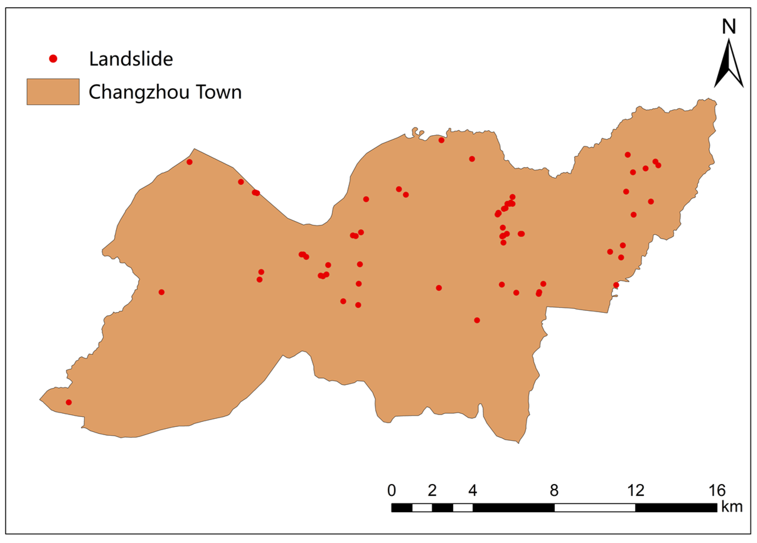
2.1. Study Area

Changzhou town, Wuzhou city, is located in the eastern part of Guangxi Province, China, at longitude 111°276549′ and latitude is 23°477830′. The administrative area of the town is 309.36 km². Changzhou town is located at the confluence of the Xunjiang and Guijiang Rivers, which form the Xijiang River after their confluence. This river traverses urban areas from west to east, and the Xunjiang, Guijiang, and Xijiang Rivers meet the Wuzhou. The terrain features are high on all sides and low in the middle, with hills accounting for more than 80% of the total area. There are many rolling hills and continuous mountains, with little flat land. The terrain slopes from north to south to the central Xijiang River and mainly consists of hills and platforms below 300 m above sea level. The Tropic of Cancer passes through Changzhou town. The area has a subtropical humid monsoon climate featuring strong solar radiation, abundant sunshine, warm temperatures, abundant rainfall, a short winter, and a long frost-free period. The average annual rainfall totals 1503.6 mm. The specific geographical location of Changzhou town is shown in Figure 1.

Overall, 65 landslides have been recorded in Changzhou town, and the distribution of landslide points is shown in Figure 2. The landslide records, physical geography data, and geological data for Changzhou town used in this paper for regional landslide susceptibility mapping were obtained from the Guangxi Zhuang Autonomous Region Geological Environment Monitoring Station.

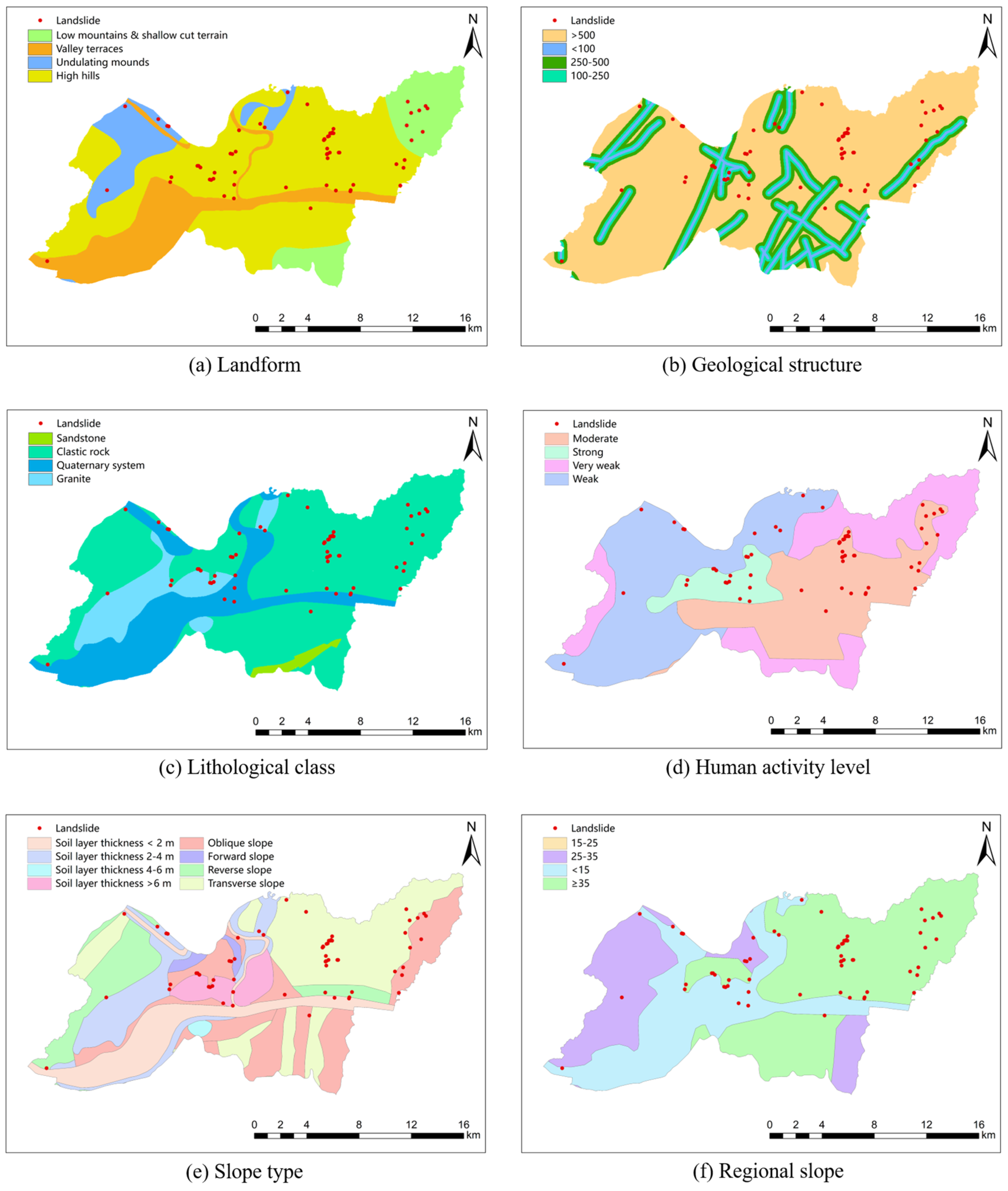
2.2. Environmental Factors

The selection of environmental factors is important in landslide susceptibility mapping, but there is no unified standard for the selection of environmental factors. In this paper, based on previous landslide susceptibility mapping results and combined with the characteristics of landslide development in Changzhou town, six landslide environmental factors, namely, landform, regional slope, geological structure, lithological class, human activity level, and slope type, were selected to perform susceptibility mapping.

In the process of landslide susceptibility mapping, it is very important to link environmental factors with known landslides [39]. The distribution and regional extent of various environmental factors are highly variable; therefore, to perform joint calculations, the various environmental factors must be unified and normalized. Since the grid method provides advantages such as regular grid shapes, a fast subdivision speed, and high modeling efficiency [10,31], this approach is selected to divide Changzhou town into grid cells. The size of each grid cell is 30 × 30 m, and there are 309,358,800 grid cells in total. In this paper, ArcGIS software is used to draw the landslide susceptibility mapping diagram. The environmental factor diagram with the six environmental factors is shown in Figure 3.

2.3. Process of Regional Landslide Susceptibility Mapping Based on the Information-GRUResNet Model

Five processes are included in the Information-GRUResNet model to generate regional landslide susceptibility maps. Figure 4 shows the complete implementation process of the model.

Step 1 The existing landslide catalog data and environmental factor data related to the landslide in Changzhou town were collected, and the obtained data were used as inputs to the landslide susceptibility mapping model.

Step 2 The initial landslide susceptibility map of Changzhou town was obtained by using the information theory method, and five evaluation grades were obtained: very low, low, moderate, high, and very high.

Step 3 The grids with the same number of landslide grids were randomly identified in each mapping level region and defined as the grid unit’s representative of each mapping level.

Step 4 The GRUResNet model was used to map the landslide susceptibility of Changzhou town by using the grid units at the very low, low, medium, and high mapping levels and the grid units for known landslides. Five kinds of mapping results were obtained.

Step 5 The GRU model, RF model, and LR model were used to generate landslide susceptibility maps for Changzhou town, and the results were compared with those of the Information-GRUResNet model.

2.4. Normalization

Before training the model, it is usually necessary to determine whether to standardize variables according to the distribution of data and map the data uniformly to the interval of [0, 1]. Normalization techniques are often effective in deep learning [40]. Normalization is an important step [41] that can accelerate the convergence speed of a network and improve the accuracy of models. In addition, the numerical intervals of various types of data will often vary, so it is necessary to normalize these data before use. The normalization formula is as follows:

$$\acute{x_i}=\frac{x_i-x_{min}}{x_{max}-x_{min}}$$

(1)

where $x_i$ represents the ith original data point, $x_{min}$ is the minimum value in the original data set, $x_{max}$ is the maximum value in the original data set, and $\acute{x_i}$ is the standardized value corresponding to the ith raw data point.

2.5. Principal Component Analysis

Principal component analysis (PCA) can be used to reduce multicollinearity in the data [42,43]. Multiple principal components are selected according to the cumulative contribution rate of each component to achieve dimension reduction. The steps are as follows:

Step 1: Suppose $n$ observed variables are $X_i=\left(x_{1i},x_{2i},\dots ,x_{Ni}\right),i=1,2,\dots ,n$, and the correlation coefficient of variables $X_s$ and $X_t\left(s,t=1,2,\dots ,n\right)$ is $r_{st}$.

Step 2: Normalize the data so that all variables are converted to the same range.

Step 3: Calculate the correlation coefficient between variables, and obtain the correlation coefficient matrix $R=\left(r_{st}\right),s,t=1,2,\dots ,n$.

Step 4: Calculate the eigenvalue ${\lambda }_i$ and the eigenvector $e_i=\left(e_{i1},e_{i2},\dots ,e_{ip}\right)$ of $R$. $\left|\left|e_i\right|\right|=1$.

Step 5: Calculate the principal component variance contribution rate (Vcr).

$$Vcr=\frac{{\lambda }_i}{{\displaystyle {\displaystyle \sum }_{i=1}^n}{\lambda }_i}$$

(2)

According to Vcr, the component with a high contribution rate can be selected to achieve the dimension reduction operation.

2.6. Information Theory

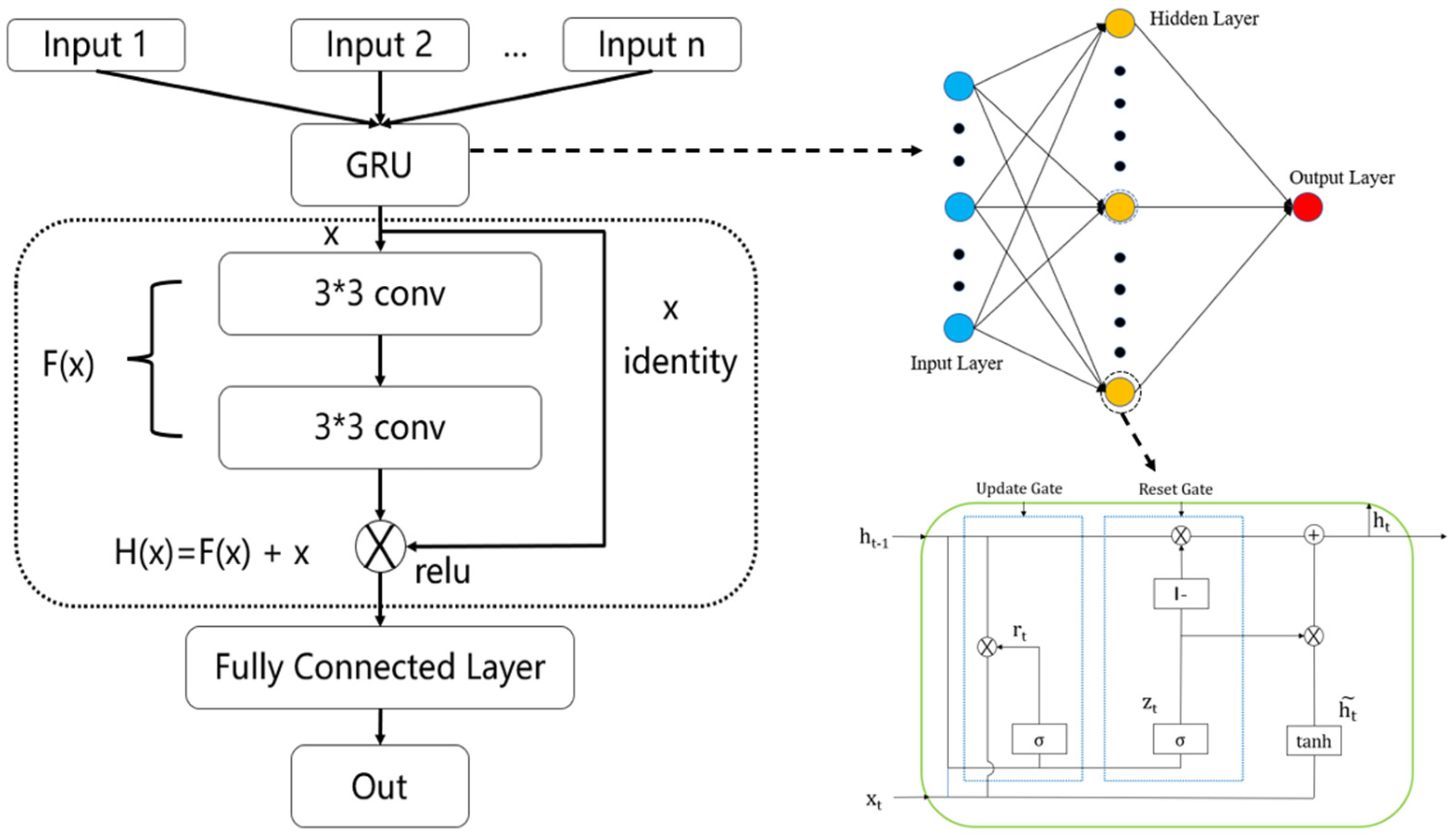
Geological hazards form via interactions among various factors. The contribution of each relevant factor to the susceptibility degree of landslide hazards can be analyzed based on information theory, which can appropriately reflect the development characteristics of geological hazards [44]. Information theory can be used to map regional landslide susceptibility [45]. Measured data for various evaluation factors that affect regional stability are converted into information that reflects regional stability. In this approach, the greater the information theory level is, the higher the landslide susceptibility [46]. Based on conditional probability, for unit $i$, the information theory level for factor $X_j$ can be expressed as:

$$I_i\left(X_j,H\right)=\ln \frac{N_j/N}{A_j/A}$$

(3)

where $N_j$ is the total number of landslide units containing factor $X_j$, $N$ is the total number of landslide units, $A_j$ is the total number of units containing factor $X_j$, and $A$ is the total number of units.

By calculating the weighted information theory level for each factor in this unit, a comprehensive landslide susceptibility mapping model is established. If $n$ factors exist in unit $i$, the summed information theory level [47] is:

$$I_i=\underset{j=1}{{\displaystyle \sum }^n}{I}_i\left(X_i,H\right)$$

(4)

2.7. GRU Model

The GRU model is an improved long short-term memory (LSTM) model that optimizes the three gate functions of LSTM, integrates the forget gate and the input gate into a single update gate [48], and mixes neuron states and hidden states, which can effectively alleviate the gradient disappearance problem in RNN networks, reduce the number of parameters in the LSTM network and is good at temporal feature extraction [49]. This approach will shorten the training time of the model. The basic structure of the GRU model is shown in Figure 5.

The GRU model includes three important components [50]: the cell state, update gate and reset gate. The cell state is the core part of the GRU. The update gate is used to determine the amount of data retained from previous memory at the current moment. The reset gate is used to determine how much past information is forgotten. The mathematical expression is as follows:

$$r_t=\sigma \left(w_r·\left[h_{t-1},x_t\right]\right)$$

(5)

$$z_t=\sigma \left(w_z·\left[h_{t-1},x_t\right]\right)$$

(6)

$${\tilde{h}}_t=\varnothing \left(w_{\tilde{h}}·\left[r_t\times h_{t-1},x_t\right]\right)$$

(7)

$$h_t=\left(\mathrm{I}-z_t\right)\times h_{t-1}+z_t\times {\tilde{h}}_t$$

(8)

$$y_t=\sigma \left(w_o·h_t\right)$$

(9)

where $x_t$ is the input vector, $h_{t-1}$ is the state memory variable at the previous moment, $h_t$ is the state memory variable at the current moment, $r_t$ is the state of the update gate, $z_t$ is the state of the reset gate, ${\tilde{h}}_t$ is the state of the current candidate set, $y_t$ is the output vector at the current time, $w_r$ is the weight of the update gate, $w_z$ is the weight of the reset gate, $w_{\tilde{h}}$ is the weight of the candidate set, $w_o$ is the weight of the output vector multiplied by the connection matrix of $x_t$ and $h_{t-1}$, $\sigma$ is the sigmoid function, $I$ is the identity matrix, $\varnothing$ is the tanh function, [] is the connection between two vectors, and $·$ is the matrix product.

2.8. ResNetGRU Model

There are many factors that influence each other during the sliding process of landslides. To further explore the coupled characteristics among landslide factors, ResNet is used to establish feature extraction units in this paper. ResNet, a new type of CNN, can enhance identity mapping to solve the degradation problem, which is of great importance for decreasing the training error in deep models. The shortcut connections in the ResNet model are the basis for saving important information and simplifying the learning target because this structure is used to directly pass the inputs to subsequent layers [51].

CNNs have been the focus of deep learning research in recent years, and as effective tools for automatic feature extraction, CNNs have been widely used in various fields. ResNet is an improved CNN and is commonly used for spatial feature extraction [51]. ResNet is generally composed of multiple stacked ResNet-block subnetworks. In this paper, the two-layer convolution basic residual unit structure is adopted, as is commonly seen in shallow networks, as shown in Figure 6.

It is assumed that the network mapping function that must be solved by ResNet-block is $H\left(x\right)$. For a general convolutional layer without a residual structure, $H\left(x\right)$ is

$$H\left(x\right)=F\left(x+w_i\right)$$

(10)

For ResNet-block with a residual structure, $H\left(x\right)$ is

$$H\left(x\right)=F\left(x+w_i\right)+x$$

(11)

In this case, the mapping function $F\left(x+w_i\right)$ learned by the convolutional network is the residual $H\left(x\right)-x$. Because residual learning is easier than the direct learning of the original features, when the residual is 0, ResNet-block is equivalent to identity mapping, and network performance is not degraded in this case; in fact, the residual is not constant at 0, and thus, ResNet-block learns new features based on the input features to improve modeling performance.

Benefitting from the advantages of the GRU model and ResNet, the ResNetGRU model with strong data feature mining ability is used in this paper to process the original data and fully explore the interactive coupled characteristics among different landslide attributes. The data processing steps of the ResNetGRU model are shown in Figure 7.

2.9. Evaluation Index

The receiver operating characteristic (ROC) curve is also called the sensitivity curve. Because of its simple and intuitive characteristics [52], it can accurately reflect the relationship between the specificity and sensitivity of the analytical method used [53] and provides good experimental accuracy; therefore, it has been widely used in landslide susceptibility mapping [15,17,21]. In the results of landslide susceptibility mapping, the abscissa represents the prediction result for a nonlandslide unit, and the ordinate represents the prediction result for a landslide unit. The ROC curve method reflects the evaluation and prediction accuracies of the model based on the area under the curve (AUC). The larger the AUC value is, the better the mapping accuracy of the model [22].

In addition to the ROC and AUC evaluation indexes often used in landslide susceptibility mapping, in this paper, the RMSE (root mean square error), MAPE (mean absolute percentage error), and MAE (mean absolute error) are also used to comprehensively evaluate the performance of the model from different perspectives. The smaller the values of these three error indexes are, the better the model performance [54].

$$MAE=\frac{1}{n}{\displaystyle \sum }_{i=1}^n\left|\widehat{y}-y_i\right|$$

(12)

$$RMSE=\sqrt{\frac{1}{n}{\displaystyle \sum }_{i=1}^n{\left({\widehat{y}}_i-y_i\right)}^2}$$

(13)

$$MAPE=\frac{100\%}{n}{\displaystyle \sum }_{i=1}^n\left|\frac{{\widehat{y}}_i-y_i}{y_i}\right|$$

(14)

where $n$ is the number of data points, $y=\left\{y_1,y_2,\dots y_n\right\}$ is the actual value, $\widehat{y}=\left\{{\widehat{y}}_1,{\widehat{y}}_2,\dots ,{\widehat{y}}_n\right\}$ is the predicted value, and $\overline{y}=\left\{{\overline{y}}_1,{\overline{y}}_2,\dots {\overline{y}}_n\right\}$ is the average value.

3. Results

3.1. Landslide Susceptibility Mapping Based on Information Theory

There are many environmental factors affecting landslide, and there may be multicollinearity in the process of factor selection because PCA can apply principal component analysis technology to extracted features to prevent multicollinearity and improve computational efficiency [42,43]. Therefore, this paper adopts the PCA method to carry out a multicollinearity analysis of environmental factors and select appropriate environmental factors.

Table 1. Contribution rate of PCA method of six environmental factors.

Landform	Geological Structure	Lithological Class	Human Activity Level	Slope Type	Regional Slope
47.43%	12.76%	9.36%	9.85%	12.2%	8.4%

shows the calculation results of the PCA method for six environmental factors.

As can be seen from Table 1, the contribution rate of the PAC method of Landform is the highest, but the proportion is not much and does not play a decisive role. While the PCA method of other factors contributes more evenly, their multicollinearity is not serious before. Therefore, from the perspective of multicollinearity, all six environmental factors are used.

In this paper, the initial landslide susceptibility mapping for Changzhou town is performed by using the information theory method. Since the final information theory value of each factor is dimensionally different, different data sets are not easy to combine or use in calculations. Thus, the data need to be normalized. The results of information theory normalization for each factor related to the occurrence of landslides are shown in

Table 2. Characteristic value and state of a landslide.

Environmental Factors	Number of Landslide Points	Total Number of Landslide Points	Number of Grids for Each Factor	Grid Area of Each Factor	Total Grid Area	Information Theory Value	Normalized Information Theory Value
Landform
High hills	8	65	200,519	180,467,100	309,358,800	−1.55599245	0.073032586
Low mountains and shallow-cut terrain	47	65	43,898	39,508,200	309,358,800	1.733753855	1
Undulating mounds	8	65	34,353	30,917,700	309,358,800	0.208227205	0.570145123
Valley terraces	2	65	64,962	58,465,800	309,358,800	−1.81518028	0
Geological structure
>500	50	65	243,989	219,590,100	309,358,800	0.080374877	0.729635056
250–500	4	65	48,020	43,218,000	309,358,800	−0.81984821	0
100–250	5	65	30,749	27,674,100	309,358,800	−0.15094454	0.542149574
<100	6	65	20,974	18,876,600	309,358,800	0.413950908	1
Lithological class
Sandstone	0	65	4903	4,412,700	309,358,800	-	-
Quaternary system	7	65	76,970	69,273,000	309,358,800	−0.73203057	0
Clastic rock	51	65	225,559	203,003,100	309,358,800	0.178718881	1
Granite	7	65	36,300	32,670,000	309,358,800	0.019567422	0.825252204
Human activity level
Very weak	1	65	86,154	77,535,600	309,358,800	−2.79062268	0
Strong	16	65	108,166	97,349,400	309,358,800	−0.24560334	0.531037444
Moderate	36	65	25,715	23,143,500	309,358,800	2.001919473	1
Weak	12	65	123,697	111,327,300	309,358,800	−0.66745336	0.443015263
Slope type
Transverse slope	26	65	108,546	97,691,400	309,358,800	0.236397506	0.705986485
Reverse slope	6	65	38,431	34,587,900	309,358,800	−0.19162994	0.347459581
Oblique slope	15	65	80,151	72,135,900	309,358,800	−0.01038714	0.499273258
Forward slope	1	65	4397	3,957,300	309,358,800	0.184552524	0.662559782
Soil layer thickness <2 m	5	65	48,490	43,641,000	309,358,800	−0.60644466	0
Soil layer thickness 2–4 m	6	65	44,161	39,744,900	309,358,800	−0.33060756	0.231048318
Soil layer thickness 4–6 m	0	65	1922	1,729,800	309,358,800	-	-
Soil layer thickness >6 m	6	65	17,634	15,870,600	309,358,800	0.587405627	1
Regional slope
<15	15	65	100,225	90,202,500	309,358,800	−0.23389244	0.583159479
25–35	5	65	75,284	67,755,600	309,358,800	−1.04635470	0
>=35	45	65	168,222	151,399,800	309,358,800	0.346852968	1
15–25	0	65	0	900	309,358,800	-	-

.

After calculations based on the information theory method, the information theory data for each grid cell are obtained, and then the results are imported into ArcGIS software. According to the natural breakpoint method [31], landslide susceptibility is divided into five levels, namely, very low, low, moderate, high, and very high, to create the landslide susceptibility map, as shown in Figure 8.

After the calculation results are divided into five levels, information such as the number of regional grids and the proportion of landslides corresponding to each susceptibility level can be calculated, as shown in

Table 3. The number of landslides corresponding to different susceptibility levels determined based on the information theory method.

Susceptibility Level	Number of Grids in the Region	Proportion of Grids (%)	Number of Landslides	Proportion of Landslides (%)
Very high	74,118	21.56	39	60
High	101,529	29.54	14	21.54
Moderate	76,771	22.33	7	10.77
Low	70,866	20.62	4	6.15
Very low	20,448	5.95	1	1.54

:

Table 3 clearly shows that there are 36 landslides in extremely prone areas, and 55.38% of the landslide grid units are in 26.61% of the total area of Changzhou town designated as having very high susceptibility to landslides. However, 73.84% of the landslide grid units in the extremely high-risk area and the high-risk area are in 50.09% of the land area, and the very low-risk area accounts for 14.38% of the total area while encompassing only 3.08% of all landslide grid units. These results indicate that the information theory method can be used to effectively evaluate the distribution characteristics of landslide susceptibility in Changzhou town.

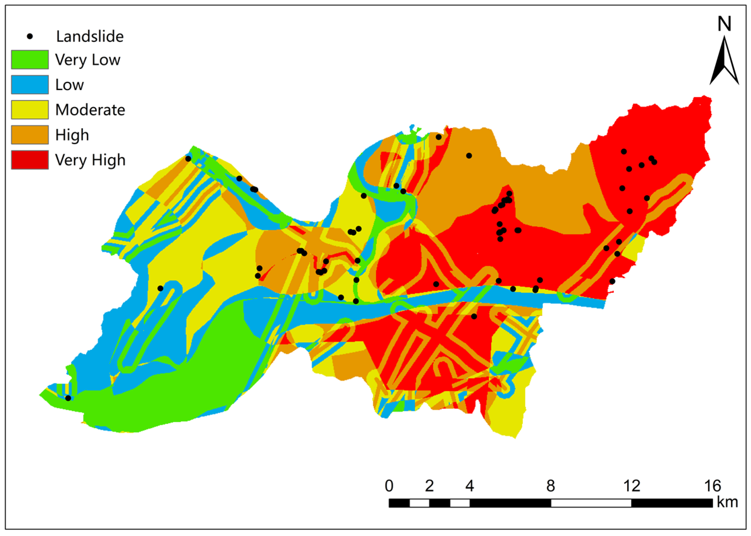
3.2. Landslide Susceptibility Mapping with the Information-GRUResNet Model

After the susceptibility results of the information theory method are obtained, grids with the same number of landslides are randomly identified from the very low, low, moderate, and high regions and defined as the grid unit’s representative of each susceptibility level. The representative grid units and the landslide grid units are used as the input variables of the Information-GRUResNet model, and the model is trained. Then, six environmental factors for each grid are used as the input variables of the model to obtain the susceptibility results for each grid unit. The grid mapping evaluation results are also divided into five grades. The Information-GRUResNet model uses the Python 3.6 runtime environment, the number of nodes in the hidden layer of the GRU model is set to 300, and the learning rate is set to 0.001. The landslide susceptibility mapping diagram of Information-GRUResNet is shown in Figure 9.

The number of regional grids and the landslide proportion information for each susceptibility level are calculated, and the results are shown in

Table 4. The number of landslides of different susceptibility levels estimated with the Information-GRUResNet model.

Susceptibility Level	Number of Grids in the Region	Proportion of Grids (%)	Number of Landslides	Proportion of Landslides (%)
Very high	74,118	21.56	39	60
High	101,529	29.54	14	21.54
Moderate	76,771	22.33	7	10.77
Low	70,866	20.62	4	6.15
Very low	20,448	5.95	1	1.54

.

As shown in Table 4, in the very high susceptibility area, 21.56% of grids occupy 60% of the total landslide area. In the very low susceptibility area, 5.95% of grids occupy 1.54% of the total landslide area. Compared with the information theory method, in this approach, the number of landslides in the very high susceptibility area increased from 36 to 39, but the proportion of grids decreased from 26.61% to 21.56%. However, 81.54% of the landslide grid units in the very high and high susceptibility areas fall within 51.1% of the total area; thus, the results of the Information-GRUResNet model include more landslides in a smaller area. This comparison indicates that the susceptibility effect of the Information-GRUResNet model is improved compared with that of the information theory method.

4. Discussion

In this paper, the original GRU model, RF model, and LR model, which are frequently used in regional landslide susceptibility mapping, are compared with the Information-GRUResNet model. Similar to the Information-GRUResNet model simulation process, the grid units representative of each susceptibility level are used as input variables to train the GRU, RF, and LR models. To ensure a consistent operating environment for the models, the GRU model adopts the same parameter settings as the Information-GRUResNet model; additionally, the number of nodes in the hidden layer of the GRU model is set to 300, and the learning rate is set to 0.001. The RF model parameters are set such that n_estimators is 10 and the gini criterion is selected, and the LR model parameters are set such that the solver is liblinear and C is 0.7. After the training of the three models, six environmental factors were input into the model at the grid level, and landslide susceptibility mapping was performed with the three models. The results of the Information-GRUResNet model and the three compared models are shown in Figure 10.

As shown in Figure 10, compared with the GRU model, the Information-GRUResNet model eliminates some very high susceptibility areas that do not contain landslide points because the ResNet model can better extract spatial features and solve the degradation problem during extraction. The effect of the RF model in very high susceptibility areas is better than that of the GRU model, but some landslide points are still missed, and the overall performance is not as good as that of the Information-GRUResNet model. In the LR results, the regions of very high susceptibility are small, considerably differing from the results of the other three models. To more intuitively compare the performance of the four models, the proportion of landslides in each susceptibility class was compared, and the results are shown in

Table 5. Number of landslides in different susceptibility levels for the Information-GRUResNet, GRU, RF, and LR models.

Susceptibility Level	Information-GRUResNet	GRU	RF	LR
Very high	39	13	24	15
High	14	33	14	34
Moderate	7	11	17	7
Low	4	6	6	8
Very low	1	2	0	1

.

The performance of these four models is similar in the very low and low susceptibility regions. The evaluation results of these four models change significantly in the moderate, high, and very high susceptibility regions. The evaluation results of the Information-GRUResNet model are relatively extreme. Most landslide points fall in very high susceptibility areas, and the number of landslide points declines with declining landslide susceptibility levels. The results of the GRU model and the LR model are similar; most of the landslide points fall in high-susceptibility areas, and there are few landslide points in very high-susceptibility areas. The RF model yields average evaluation results. Although the number of landslide points within very high susceptibility areas is the largest, the number is not much, and the number of landslide points in moderate susceptibility areas is greater than that in high susceptibility areas. As shown in Table 5, the Information-GRUResNet model yields the best evaluation effect. Although the other three models yield reasonable results, the results of the GRU and LR models do not reflect the locations of most landslide points, and the results of the RF model do not appropriately reflect extreme cases. In general, the evaluation results of the Information-GRUResNet model are the most similar to the actual conditions in Changzhou town.

The performance evaluation indexes discussed above can be used to objectively compare the performance of the four models of landslide susceptibility mapping. The ROC and AUC evaluation results are shown in Figure 11.

As shown in Figure 11, the Information-GRUResNet model yields the best evaluation effect, and the corresponding AUC value exceeds 0.8, indicating that the Information-GRUResNet model achieves excellent results in landslide susceptibility mapping for Changzhou town. Since Information-GRUResNet and the GRU, RF, and LR models are all neural network models, the RMSE, MAE, and MAPE are introduced to evaluate their performance. The results of these three evaluation indicators are shown in

Table 6. Evaluation index results for the Information-GRUResNet, GRU, RF, and LR models.

Model	MSE	MAE	RMSE
Information-GRUResNet	1.32307692	0.83076923	1.15025081
GRU	1.67692308	1.01	1.29496065
RF	2.13846154	1.09230769	1.46234795
LR	1.89230769	1.03076923	1.37561175

.

Similar to the results in Figure 11, the GRUResNet model values of the three error evaluation indexes are all the minimum, which indicates that the deviation between its evaluation value and the real value is the minimum, and the evaluation effect is the best among the four models. GRU model has a better evaluation effect than RF and LR models because it can deal with the nonlinear relationship between landslide and disaster-bearing environmental factors well and the extraction temporal characteristics. In order to represent this comparative study clearly, we also use present a Taylor diagram [55], as shown in Figure 12.

Taylor diagram can show standard deviation, correlation coefficient, and RMSE simultaneously [56]. The results in Figure 12 also show that the Information-GRUResNet model is superior. In summary, the results of the GRUResNet model are closer to the actual situation of Changzhou town, which successfully realizes the landslide susceptibility mapping of Changzhou town.

5. Conclusions

In this study, Changzhou town, Wuzhou city, Southwest China, is selected as the research area, and six environmental factors, namely, landform, regional slope, geological structure, lithological class, human activity level, and slope type, are combined with existing landslide records to establish a deep learning Information-GRUResNet model for landslide susceptibility mapping. The model fully considers the nonlinear relationships between landslides and environmental factors and can extract the relevant temporal and spatial characteristics of the data, effectively solving the problems of the random selection of nonlandslide points in the susceptibility evaluation process and gradient disappearance, explosion, and degradation in general deep learning models. This model uses the information theory approach, which requires no training in advance, to construct the initial landslide susceptibility map and obtain a grid unit representation of each area. This approach solves the problem of randomly selecting nonlandslide units. Then, the GRUResNet model is used to construct the final landslide susceptibility mapping evaluation results. Finally, the model is compared with the GRU, RF, and LR models. The conventional ROC and AUC indexes and the RMSE, MAE, and MAPE are applied to compare the results. The simulation results verify the effectiveness of the Information-GRUResNet model in landslide susceptibility mapping. This model can effectively improve decision-makers’ judgments regarding the regional landslide occurrence probability and aid in identifying high-risk landslide areas and predicting loss of life and property caused by landslides. Moreover, the model is easy to customize and can be quickly applied for landslide susceptibility mapping in other areas.

References

1. Chao, Z.; Kunlong, Y.; Ying, C.; Bayes, A. Application of time series analysis and PSO–SVM model in predicting the Bazimen landslide in the Three Gorges Reservoir, China. Eng. Geol. 2016, 204, 108–120. [Google Scholar]
2. Yonggang, Z.; Jun, T.; Zhengying, H.; Junkun, T. A novel displacement prediction method using gated recurrent unit model with time series analysis in the Erdaohe landslide. Nat. Hazards 2021, 105, 783–813. [Google Scholar]
3. Xiuzhen, L.; Shengwei, L. Large-Scale Landslide Displacement Rate Prediction Based on Multi-Factor Support Vector Regression Machine. Appl. Sci. 2021, 11, 1381. [Google Scholar]
4. Shaohong, L.; Na, W. A new grey prediction model and its application in landslide displacement prediction. Chaos Solitons Fractals 2021, 147, 110969. [Google Scholar]
5. Yong, Z.; Zhengwei, Z.; Wanjie, L.D.G.; Wang, X. Experimental research on a novel optic fiber sensor based on OTDR for landslide monitoring. Measurement 2019, 148, 106926. [Google Scholar]
6. Junwei, M.; Huiming, T.; Xiao, L.; Tao, W.; Junrong, Z.; Qinwen, T.; Zhiqiang, F. Probabilistic forecasting of landslide displacement accounting for epistemic uncertainty: A case study in the Three Gorges Reservoir area, China. Landslides 2018, 15, 1145–1153. [Google Scholar]
7. Shiluo, X.; Ruiqing, N. Displacement prediction of Baijiabao landslide based on empirical mode decomposition and long short-term memory neural network in Three Gorges area, China. Comput. Geosci. 2018, 111, 87–96. [Google Scholar]
8. Richard, M.; Lanhai, L.; Jean, B.N.; Christophe, M.; Enan, M.N.; Patient, M.K.; Aboubakar, G.; Egide, H. Landslide susceptibility and influencing factors analysis in Rwanda. Environ. Dev. Sustain. 2020, 22, 7985–8012. [Google Scholar]
9. Andrea, C.; Federico, R.; Daniela, L.; Filippo, C.; Nicola, C. Landslide susceptibility map refinement using PSInSAR data. Remote Sens. Environ. 2016, 184, 302–315. [Google Scholar]
10. Xing, A.-Z.; Yamin, M.; Rongxun, W.; Tongxin, Z.; Yongcui, D.; Junzhi, L.; Lin, Y.; Cheng-Zhi, Q.; Haoyuan, H. A comparative study of an expert knowledge-based model and two data-driven models for landslide susceptibility mapping. Catena 2018, 166, 317–327. [Google Scholar]
11. Rubini, M.; Olsen, J.M. Evaluation of the influence of source and spatial resolution of DEMs on derivative products used in landslide mapping. Geomat. Nat. Hazards Risk 2015, 7, 1835–1855. [Google Scholar]
12. Qingfeng, H.; Himan, S.; Ataollah, S.; Shaojun, L.; Wei, C.; Nianqin, W.; Huichan, C.; Huiyuan, B.; Jianquan, M.; Yingtao, C.; et al. Landslide spatial modelling using novel bivariate statistical based Naïve Bayes, RBF Classifier, and RBF Network machine learning algorithms. Sci. Total Environ. 2019, 663, 1–15. [Google Scholar]
13. Vakhshoori, V.; Zare, M. Landslide susceptibility mapping by comparing weight of evidence, fuzzy logic, and frequency ratio methods. Geomat. Nat. Hazards Risk 2016, 7, 1731–1752. [Google Scholar] [CrossRef]
14. Guo-liang, D.; Yong-shuang, Z.; Javed, I.; Zhi-hua, Y.; Xin, Y. Landslide susceptibility mapping using an integrated model of information value method and logistic regression in the Bailongjiang watershed, Gansu Province, China. J. Mt. Sci. 2017, 2, 249–268. [Google Scholar]
15. Haoyuan, H.; Paraskevas, T.; Ioanna, I.; Constantinos, L.; Yi, W. Introducing a novel multi-layer perceptron network based on stochastic gradient descent optimized by a meta-heuristic algorithm for landslide susceptibility mapping. Sci. Total Environ. 2020, 742, 140549. [Google Scholar]
16. Qian, W.; Yi, W.; Ruiqing, N.; Ling, P. Integration of Information Theory, K-Means Cluster Analysis and the Logistic Regression Model for Landslide Susceptibility Mapping in the Three Gorges Area, China. Remote Sens. 2017, 9, 938. [Google Scholar]
17. Taskin, K.; Emrehan, K.S.; Ismail, C. An assessment of multivariate and bivariate approaches in landslide susceptibility mapping: A case study of Duzkoy district. Nat. Hazards 2015, 76, 471–496. [Google Scholar]
18. Wenhuan, W.; Qiang, Z.; Vijay, P.S.; Gang, W.; Jiaqi, Z.; Zexi, S.; Shuai, S. A Data-Driven Model on Google Earth Engine for Landslide Susceptibility Assessment in the Hengduan Mountains, the Qinghai–Tibetan Plateau. Remote Sens. 2022, 14, 4662. [Google Scholar]
19. Prakash, N.; Manconi, A.; Loew, S. Mapping Landslides on EO Data: Performance of Deep Learning Models vs. Traditional Machine Learning Models. Remote Sens. 2020, 12, 346. [Google Scholar] [CrossRef] [Green Version]
20. Thomas, S.; Dalia, B.K. A heuristic approach to global landslide susceptibility mapping. Nat. Hazards 2017, 87, 145–164. [Google Scholar]
21. Jie, D.; Ali, P.Y.; Dieu, T.B.; Abdelaziz, M.; Mehebub, S.; Zhongfan, Z.; Chi-Wen, C.; Khabat, K.; Yong, Y.; Binh, T.P. Assessment of advanced random forest and decision tree algorithms for modeling rainfall-induced landslide susceptibility in the Izu-Oshima Volcanic Island, Japan. Sci. Total Environ. 2019, 662, 332–346. [Google Scholar]
22. Vahid, M.; Yaghoub, N. Development of hybrid wavelet packet-statistical models (WP-SM) for landslide susceptibility mapping. Landslides 2016, 13, 97–114. [Google Scholar]
23. Wei, C.; Hamid, R.P.; Zhou, Z. A GIS-based comparative study of Dempster-Shafer, logistic regression and artificial neural network models for landslide susceptibility mapping. Geocarto Int. 2016, 32, 367–385. [Google Scholar]
24. Wei, C.; Wenping, L.; Huichan, C.; Enke, H.; Xiaoqin, L.; Xiao, D. GIS-based landslide susceptibility mapping using analytical hierarchy process (AHP) and certainty factor (CF) models for the Baozhong region of Baoji City, China. Environ. Earth Sci. 2016, 75, 63. [Google Scholar]
25. Xianyu, Y.; Kaixiang, Z.; Yingxu, S.; Weiwei, J.; Jianguo, Z. Study on landslide susceptibility mapping based on rock–soil characteristic factors. Sci. Rep. 2021, 11, 15476. [Google Scholar]
26. Paraskevas, T.; Ioanna, I. Comparison of a logistic regression and Naïve Bayes classifier in landslide susceptibility assessments: The influence of models complexity and training dataset size. Catena 2016, 145, 164–179. [Google Scholar]
27. Mahdi, P.; Amiya, G.; Hamid, R.P.; Fatemeh, R.; Saro, L. Spatial prediction of landslide susceptibility using hybrid support vector regression (SVR) and the adaptive neuro-fuzzy inference system (ANFIS) with various metaheuristic algorithms. Sci. Total Environ. 2020, 741, 139937. [Google Scholar]
28. Mohammad, F.; Alireza, V.; Ali, A.A.; Mahdi, M.; Hossein, A. Mapping landslide susceptibility in the Zagros Mountains, Iran: A comparative study of different data mining models. Earth Sci. Inform. 2019, 12, 615–628. [Google Scholar]
29. Krzysztof, G.; María, T.R. The importance of input data on landslide susceptibility mapping. Sci. Rep. 2021, 11, 19334. [Google Scholar]
30. Abdelaziz, M.; Ali, P.Y.; Jie, D.; Jim, W.; Binh, T.; Dieu, T.B.; Ram, A.; Boumezbeur, A. Machine learning methods for landslide susceptibility studies: A comparative overview of algorithm performance. Earth-Sci. Rev. 2020, 207, 103225. [Google Scholar]
31. Faming, H.; Jing, Z.; Chuangbing, Z.; Yuhao, W.; Jinsong, H.; Li, Z. A deep learning algorithm using a fully connected sparse autoencoder neural network for landslide susceptibility prediction. Landslides 2020, 17, 217–229. [Google Scholar]
32. Yanting, P.; Yaping, H.; Qi, Z.; Xingyuan, Z.; Song, W. Effects of Image Degradation and Degradation Removal to CNN-Based Image Classification. IEEE Trans. Pattern Anal. Mach. Intell. 2021, 43, 1239–1253. [Google Scholar]
33. Yaning, Y.; Zhijie, Z.; Wanchang, Z.; Huihui, J.; Jianqiang, Z. Landslide susceptibility mapping using multiscale sampling strategy and convolutional neural network: A case study in Jiuzhaigou region. Catena 2020, 195, 104851. [Google Scholar]
34. Zhice, F.; Yi, W.; Ling, P.; Haoyuan, H. Integration of convolutional neural network and conventional machine learning classifiers for landslide susceptibility mapping. Comput. Geosci. 2020, 139, 104470. [Google Scholar]
35. Somnath, B.; Vaibhav, K.U.; Balamurugan, G.; Thomas, O. Landslide inventory and susceptibility models considering the landslide typology using deep learning: Himalayas, India. Nat. Hazards 2021, 108, 1257–1289. [Google Scholar]
36. Weidong, W.; Zhuolei, H.; Zheng, H.; Yange, L.; Jie, D.; Jianling, H. Mapping the susceptibility to landslides based on the deep belief network: A case study in Sichuan Province, China. Nat. Hazards 2020, 103, 3239–3261. [Google Scholar]
37. Phuong, T.T.; Mahdi, P.; Khabat, K.; Omid, G.; Narges, K.; Artemi, C.; Saro, L. Evaluation of deep learning algorithms for national scale landslide susceptibility mapping of Iran. Geosci. Front. 2021, 12, 505–519. [Google Scholar]
38. Maher, I.S.; Biswajeet, P.; Saro, L. Application of convolutional neural networks featuring Bayesian optimization for landslide susceptibility assessment. Catena 2020, 186, 104249. [Google Scholar]
39. Faming, H.; Kunlong, Y.; Jinsong, H.; Lei, G.; Peng, W. Landslide susceptibility mapping based on self-organizing-map network and extreme learning machine. Eng. Geol. 2017, 223, 11–22. [Google Scholar]
40. Ping, L.; Ruimao, Z.; Jiamin, R.; Zhanglin, P.; Jingyu, L. Switchable Normalization for Learning-to-Normalize Deep Representation. IEEE Trans. Pattern Anal. Mach. Intell. 2019, 43, 712–728. [Google Scholar]
41. Zhaodong, C.; Lei, D.; Guoqi, L.; Jiawei, S. Effective and Efficient Batch Normalization Using a Few Uncorrelated Data for Statistics Estimation. IEEE Trans. Neural Netw. Learn. Syst. 2020, 32, 348–362. [Google Scholar]
42. Furkan, E.; Özgün, Y.; Ali, Y.M. Predictive modeling of biomass gasification with machine learning-based regression methods. Energy 2020, 191, 116541. [Google Scholar]
43. Douglas, M.C.; Ana, P.F.; Brivaldo, G.A.; Fernando, J.F.; dos Santos Silva, T.H.; Silva Cavalcante, F.M. Physical soil quality indicators for environmental assessment and agricultural potential of Oxisols under different land uses in the Araripe Plateau, Brazil. Soil Tillage Res. 2021, 209, 104951. [Google Scholar]
44. Zhihua, Y.; Hengxing, L.; Xing, G.; Langping, L.; Yunshan, M.; Yuming, W. Urgent landslide susceptibility assessment in the 2013 Lushan earthquake-impacted area, Sichuan Province, China. Nat. Hazards 2015, 75, 2467–2487. [Google Scholar]
45. Paraskevas, T.; Ioanna, I.; Haoyuan, H.; Wei, C.; Chong, X. Applying information theory and GIS-based quantitative methods to produce landslide susceptibility maps in Nancheng County, China. Landslide 2017, 14, 1091–1111. [Google Scholar]
46. Hamid, R.P.; Majid, M.; Biswajeet, P. Landslide susceptibility mapping using index of entropy and conditional probability models in GIS: Safarood Basin, Iran. Catena 2012, 97, 71–84. [Google Scholar]
47. Krishna, C.D.; Amar, D.R.; Hamid, R.P.; Kohki, Y.; Biswajeet, P.; In, C.R.; Megh, R.D.; Omar, F. Althuwaynee. Landslide susceptibility mapping using certainty factor, index of entropy and logistic regression models in GIS and their comparison at Mugling–Narayanghat road section in Nepal Himalaya. Nat. Hazards 2013, 65, 135–165. [Google Scholar]
48. Chuxiong, H.; Tiansheng, O.; Yu, Z.; LiMin, Z. GRU-Type LARC Strategy for Precision Motion Control with Accurate Tracking Error Prediction. IEEE Trans. Ind. Electron. 2020, 68, 812–820. [Google Scholar]
49. Jin, W.; You, Z.; LiangChih, Y.; Xuejie, Z. Contextual sentiment embeddings via bi-directional GRU language model. Knowl.-Based Syst. 2022, 235, 107663. [Google Scholar]
50. Yaxiong, W.; Zhenhang, C.; Wei, Z. Lithium-ion battery state-of-charge estimation for small target sample sets using the improved GRU-based transfer learning. Energy 2022, 244, 123178. [Google Scholar]
51. Zhimin, L.; Shaobing, Y.; Yuanzhong, W.; Jinyu, Z. Discrimination of the fruits of Amomum tsao-ko according to geographical origin by 2DCOS image with RGB and Resnet image analysis techniques. Microchem. J. 2021, 169, 106545. [Google Scholar]
52. Stephan, F.; Jesse, G. Defining the extent of gene function using ROC curvature. Stephan Fischer. Bioinformatics 2022, 38, 5390–5397. [Google Scholar]
53. Sadatsafavi, M.; Saha-Chaudhuri, P.; Petkau, J. Model-Based ROC Curve: Examining the Effect of Case Mix and Model Calibration on the ROC Plot. Med. Decis. Mak. 2022, 42, 487–499. [Google Scholar] [CrossRef]
54. Lin, Z.; Sun, X.; Ji, Y. Landslide Displacement Prediction based on Time Series Analysis and Double-BiLSTM Model. Int. J. Enviromental Res. Public Health 2022, 19, 2077. [Google Scholar] [CrossRef] [PubMed]
55. Taylor, K.E. Summarizing multiple aspects of model performance in a single diagram. J. Geophys. Res. Atmos. 2001, 106, 7183–7192. [Google Scholar] [CrossRef]
56. Lucy, R.W.; Alessandra, M.; Malcolm, H.; Moninya, R.; Craig, R.S. Assessment of surface currents measured with high-frequency phased-array radars in two regions of complex circulation. IEEE J. Ocean. Eng. 2017, 43, 484–505. [Google Scholar]
Figure 1. Specific geographical location of Changzhou town.
Forests 14 00499 g001
Figure 2. Distribution of landslide points in Changzhou town.
Forests 14 00499 g002
Figure 3. Environmental factor diagram for Changzhou town.
Forests 14 00499 g003
Figure 4. Process of regional landslide susceptibility mapping based on the Information-GRUResNet model.
Forests 14 00499 g004
Figure 5. This is a figure. Schemes follow the same formatting.
Forests 14 00499 g005
Figure 6. Residual block structure.
Forests 14 00499 g006
Figure 7. ResNetGRU model structure.
Forests 14 00499 g007
Figure 8. Landslide susceptibility mapping results based on information theory.
Forests 14 00499 g008
Figure 9. Landslide susceptibility mapping results based on the Information-GRUResNet model.
Forests 14 00499 g009
Figure 10. Comparison of the landslide susceptibility mapping results of Information-GRUResNet and the GRU, RF, and LR models.
Forests 14 00499 g010
Figure 11. Comparison of the ROC and AUC results for the Information-GRUResNet, GRU, RF, and LR models.
Forests 14 00499 g011
Figure 12. Comparison of the ROC and AUC results for the Information-GRUResNet, GRU, RF, and LR models.
Forests 14 00499 g012