
Species Distribution Modelling under Climate Change Scenarios for Maritime Pine (Pinus pinaster Aiton) in Portugal
 , ,
, ,  , and
, and 
Abstract
:1. Introduction
2. Materials and Methods
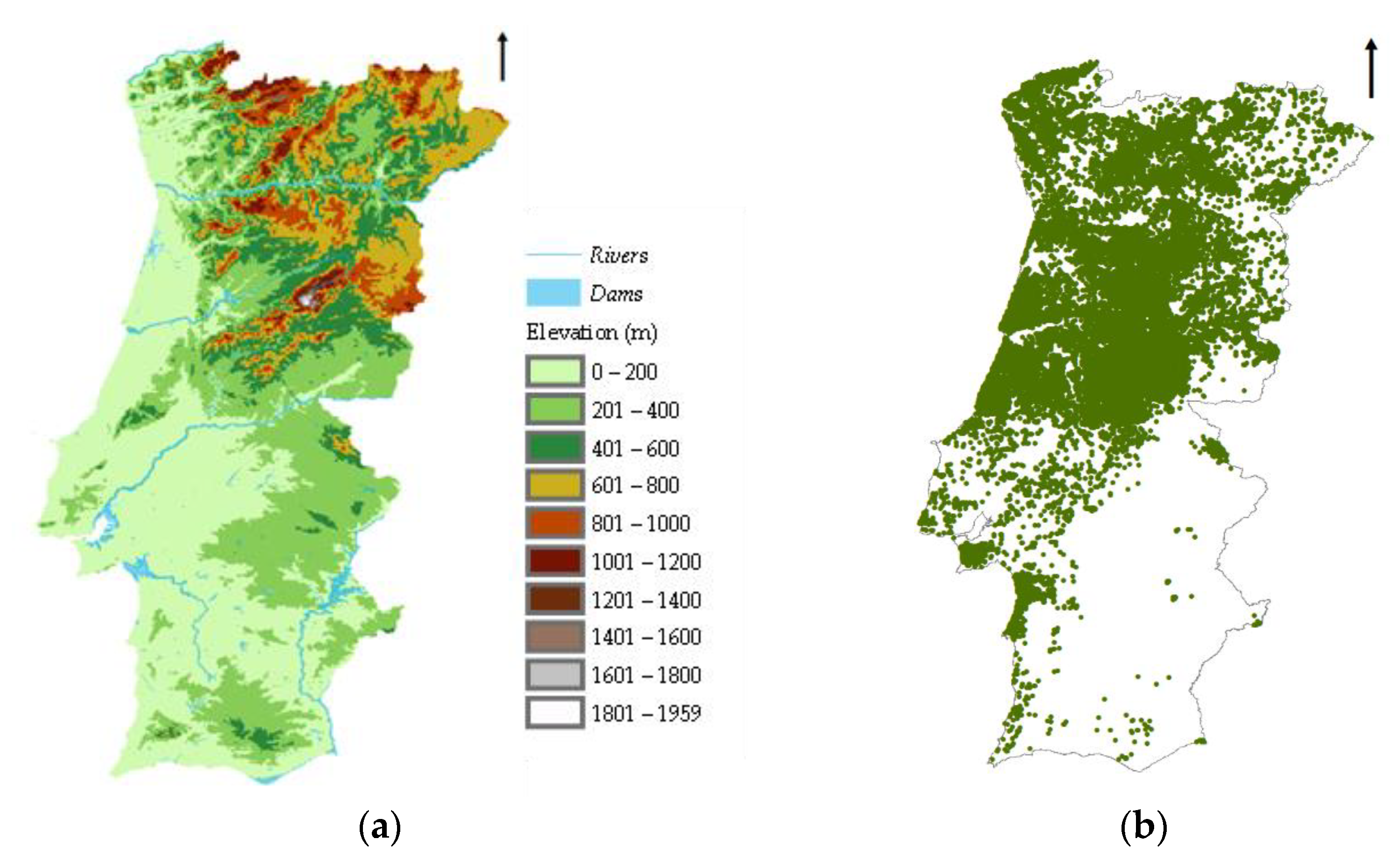
2.1. Study Area
2.2. Data
2.2.1. Species Occurrence Data
2.2.2. Environmental Data
2.3. Methods
2.3.1. MaxEnt Modelling Approach
2.3.2. Ecological Envelope Approach
2.3.3. Methodological Approaches Agreement Analysis
3. Results
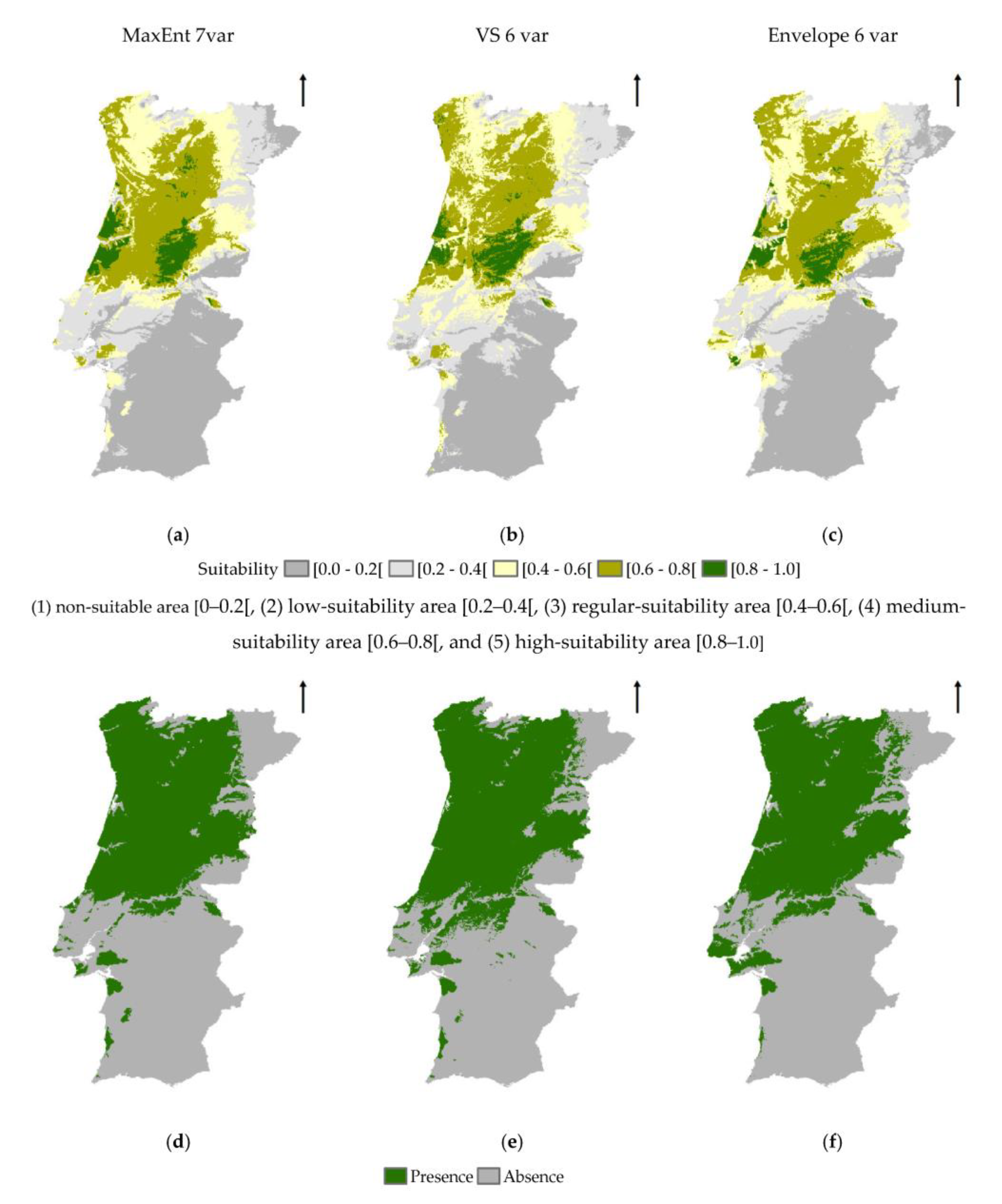
3.1. MaxEnt Modelling Approach
3.1.1. Explanatory Variables Selection
3.1.2. MaxEnt Model
3.2. Ecological Envelope Approach
3.3. Methodological Approaches Agreement Analysis
4. Discussion
5. Conclusions
Author Contributions
Funding
Conflicts of Interest
References
- Pecchi, M.; Marchi, M.; Burton, V.; Giannetti, F.; Moriondo, M.; Bernetti, I.; Bindi, M.; Chirici, G. Species distribution modelling to support forest management. A literature review. Ecol. Modell. 2019, 411, 108817. [Google Scholar] [CrossRef]
- Alegria, C.; Roque, N.; Albuquerque, T.; Gerassis, S.; Fernandez, P.; Ribeiro, M.M. Species ecological envelopes under climate change scenarios: A case study for the main two wood-production forest species in Portugal. Forests 2020, 11, 880. [Google Scholar] [CrossRef]
- Barrio-Anta, M.; Castedo-Dorado, F.; Cámara-Obregón, A.; López-Sánchez, C.A. Predicting current and future suitable habitat and productivity for Atlantic populations of maritime pine (Pinus pinaster Aiton) in Spain. Ann. For. Sci. 2020, 77, 41. [Google Scholar] [CrossRef]
- De Rivera, Ó.R.; López-Quílez, A.; Blangiardo, M. Assessing the spatial and spatio-temporal distribution of forest species via Bayesian hierarchical modeling. Forests 2018, 9, 573. [Google Scholar] [CrossRef] [Green Version]
- Phillips, S.J.; Anderson, R.P.; Schapire, R.E. Maximum entropy modeling of species geographic distributions. Ecol. Modell. 2006, 190, 231–259. [Google Scholar] [CrossRef] [Green Version]
- Jinga, P.; Liao, Z.; Nobis, M.P. Species distribution modeling that overlooks intraspecific variation is inadequate for proper conservation of marula (Sclerocarya birrea, Anacardiaceae). Glob. Ecol. Conserv. 2021, 32, e01908. [Google Scholar] [CrossRef]
- Khan, A.M.; Li, Q.; Saqib, Z.; Khan, N.; Habib, T.; Khalid, N.; Majeed, M.; Tariq, A. MaxEnt Modelling and Impact of Climate Change on Habitat Suitability Variations of Economically Important Chilgoza Pine (Pinus gerardiana Wall.) in South Asia. Forests 2022, 13, 715. [Google Scholar] [CrossRef]
- Engel, M.; Mette, T.; Falk, W. Spatial species distribution models: Using Bayes inference with INLA and SPDE to improve the tree species choice for important European tree species. For. Ecol. Manag. 2022, 507, 119983. [Google Scholar] [CrossRef]
- Soberón, J. Grinnellian and Eltonian niches and geographic distributions of species. Ecol. Lett. 2007, 10, 1115–1123. [Google Scholar] [CrossRef]
- Peterson, A.T.; Soberón, J. Species distribution modeling and ecological niche modeling: Getting the Concepts Right. Nat. Conserv. 2012, 10, 102–107. [Google Scholar] [CrossRef]
- Hijmans, R.; Cameron, S.; Parra, J.; Jones, P.; Jarvis, A. Very High Resolution Interpolated Climate Surfaces for Global Land Areas. Int. J. Climatol. 2005, 25, 1965–1978. [Google Scholar] [CrossRef]
- Alegria, C.; Roque, N.; Albuquerque, T.; Fernandez, P.; Ribeiro, M.M. Modelling maritime pine (Pinus pinaster aiton) spatial distribution and productivity in Portugal: Tools for forest management. Forests 2021, 12, 368. [Google Scholar] [CrossRef]
- Ribeiro, M.M.; Roque, N.; Ribeiro, S.; Gavinhos, C.; Castanheira, I.; Quinta-Nova, L.; Albuquerque, T.; Gerassis, S. Bioclimatic modeling in the Last Glacial Maximum, Mid-Holocene and facing future climatic changes in the strawberry tree (Arbutus unedo L.). PLoS ONE 2019, 14, e0210062. [Google Scholar] [CrossRef] [PubMed] [Green Version]
- Almeida, A.M.; Martins, M.J.; Campagnolo, M.L.; Fernandez, P.; Albuquerque, T.; Gerassis, S.; Gonçalves, J.C.; Ribeiro, M.M. Prediction scenarios of past, present, and future environmental suitability for the Mediterranean species Arbutus unedo L. Sci. Rep. 2022, 12, 84. [Google Scholar] [CrossRef]
- Elith, J.H.; Graham, C.P.H.; Anderson, R.P.; Dudík, M.; Ferrier, S.; Guisan, A.; Hijmans, R.J.; Huettmann, F.; Leathwick, J.R.; Lehmann, A.; et al. Novel methods improve prediction of species’ distributions from occurrence data. Ecography 2006, 29, 129–151. [Google Scholar] [CrossRef] [Green Version]
- Albuquerque, J. Carta Ecológica de Portugal; Ministério da Economia, Direcção Geral dos Serviços Agrícolas, Repartição de Estudos, Informação e Propaganda: Lisboa, Portugal, 1954. (In Portuguese) [Google Scholar]
- DGRF. Plano Regional de Ordenamento Florestal do Pinhal Interior Sul. Documento Estratégico; Direção Geral dos Recursos Florestais: Lisboa, Portugal, 2005; 603p. (In Portuguese) [Google Scholar]
- Quinta-Nova, L.; Roque, N.; Navalho, I.; Alegria, C.; Albuquerque, T. Using geostatistics and multicriteria spatial analysis to map forest species biogeophysical suitability: A study case for the Centro region of Portugal. In Information and Communication Technologies in Modern Agricultural Development; Salampasis, M., Bournaris, T., Eds.; Springer International Publishing: Cham, Switzerland, 2019; pp. 64–83. ISBN 978-3-030-12998-9. [Google Scholar]
- Alves, A.M.; Pereira, J.S.; Correia, V. Silvicultura. A Gestão dos Ecossistemas Florestais; Fundação Calouste Gulbenkian: Lisboa, Portugal, 2012; 597p. (In Portuguese) [Google Scholar]
- Aguiar, C.; Capelo, J.; Catry, F. Distribuição dos pinhais em Portugal. In Pinhais e Eucaliptais. Árvores e Florestas de Portugual; Silva, J., Ed.; Público, Comunicação Social, S.A., Fundação Luso-Americana para o Desenvolvimento: Lisboa, Portugal, 2007; pp. 89–104. (In Portuguese) [Google Scholar]
- Navalho, I.; Alegria, C.; Quinta-Nova, L.; Fernandez, P. Integrated planning for landscape diversity enhancement, fire hazard mitigation and forest production regulation: A case study in central Portugal. Land Use Policy 2017, 61, 398–412. [Google Scholar] [CrossRef]
- Dias, S.S.; Ferreira, A.G.; Gonçalves, A.C.; Cristina, B.C. Definição de zonas de aptidão para espécies florestais com base em características edafo-climáticas. Silva Lusit. 2008, 16, 17–35. (In Portuguese) [Google Scholar]
- Navalho, I.; Alegria, C.; Roque, N.; Quinta-Nova, L. Mapping forest landscape multifunctionality using multicriteria spatial analysis. Floresta e Ambient. 2019, 26. [Google Scholar] [CrossRef] [Green Version]
- Mesquita, S.; Capelo, J. Cartografia de Aptidão Bioclimática ao Pinheiro-Bravo (Pinus pinaster Aiton) Para Portugal Continental. LEAF/ISA/ULisboa. Available online: http://epic-webgis-portugal.isa.utl.pt/ (accessed on 21 June 2022).
- Pereira, J.S.; Correia, A.V.; Correia, C.V.; Ferreira, M.T.; Onofre, N.; Freitas, H.; Godinho, F. Florestas e biodiversidade. In Alterações Climáticas em Portugal. Cenários, Impactos e Medidas de Adaptação (Projecto SIAM II); Santos, F., Miranda, P.M., Eds.; Gradiva: Lisboa, Portugal, 2006; pp. 301–344. (In Portuguese) [Google Scholar]
- Costa, R.; Fraga, H.; Fernandes, P.M.; Santos, J.A. Implications of future bioclimatic shifts on Portuguese forests. Reg. Environ. Chang. 2017, 17, 117–127. [Google Scholar] [CrossRef]
- ICNF. 6o Inventário Florestal Nacional—IFN6. 2015. Relatório Final; Instituto da Conservação da Natureza e das Florestas: Lisboa, Portugal, 2019; 284p, Available online: https://www.icnf.pt/api/file/doc/c8cc40b3b7ec8541 (accessed on 24 February 2023). (In Portuguese)
- AFN Inventário Florestal Nacional Portugal Continental. 5o Inventário Florestal Nacional 2005–2006. FloreStat—Aplicação. Autoridade Florestal Nacional. Lisboa, Portugal. 2010. Available online: https://www.icnf.pt/florestas/flestudosdocumentosestatisticasindicadores (accessed on 24 February 2023). (In Portuguese).
- DGRF. Inventário Florestal Nacional Portugal Continental. 3a Revisão, 1995–1998. Relatório Final; Direção-Geral dos Recursos Florestais: Lisboa, Portugal, 2010; Available online: https://www.icnf.pt/florestas/flestudosdocumentosestatisticasindicadores (accessed on 24 February 2023). (In Portuguese)
- AFN Inventário Florestal Nacional Portugal Continental. 5o Inventário Florestal Nacional 2005–2006. Apresentação do relatório final; Autoridade Florestal Nacional: Lisboa, Portugal, 2010; Available online: https://www.icnf.pt/florestas/flestudosdocumentosestatisticasindicadores (accessed on 24 February 2023). (In Portuguese)
- Moreira, F.; Viedma, O.; Arianoutsou, M.; Curt, T.; Koutsias, N.; Rigolot, E.; Barbati, A.; Corona, P.; Vaz, P.; Xanthopoulos, G.; et al. Landscape—Wildfire interactions in southern Europe: Implications for landscape management. J. Environ. Manag. 2011, 92, 2389–2402. [Google Scholar] [CrossRef] [Green Version]
- Alegria, C.; Pedro, N.; do Carmo Horta, M.; Roque, N.; Fernandez, P. Ecological envelope maps and stand production of eucalyptus plantations and naturally regenerated maritime pine stands in the central inland of Portugal. For. Ecol. Manag. 2019, 432, 327–344. [Google Scholar] [CrossRef]
- IPMA Clima de Portugal Continental. Available online: https://www.ipma.pt/pt/educativa/tempo.clima/ (accessed on 24 February 2023).
- Oliveira, A. Boas Práticas Florestais Para o Pinheiro-Bravo. Manual; Pinus, C., Ed.; Centro PINUS: Porto, Portugal, 1999; Available online: https://centropinus.org/files/2018/04/manual01.pdf (accessed on 24 February 2023). (In Portuguese)
- Fonseca, T.F.; Gonçalves, A.C.; Lousada, J. Maritime Pine, Its Biological and Silvicultural Traits for the Basis of Natural Resources: An Overview; Gonçalves, A.C., Fonseca, T., Eds.; IntechOpen: Rijeka, Croatia, 2022; p. Ch. 1. ISBN 978-1-83969-777-7. [Google Scholar]
- DGT. Especificações Técnicas da Carta de Uso e Ocupação do Solo de Portugal Continental Para 1995, 2007, 2010 e 2015; Relatório Técnico; Direção-Geral do Território: Lisboa, Portugal, 2018; Available online: http://www.dgterritorio.pt/cartografia_e_geodesia/cartografia/cartografia_tematica/cartografia_de_uso_e_ocupacao_do_solo__cos_clc_e_copernicus_/ (accessed on 24 February 2023). (In Portuguese)
- DGT. Carta de Uso e Ocupação do solo. Registo Nacional de dados Geográficos. SNIG. Direção-Geral do Território. Lisboa. Portugal. Available online: https://snig.dgterritorio.gov.pt/rndg/srv/por/catalog.search#/search?anysnig=COS&fast=index (accessed on 24 February 2023). (In Portuguese)
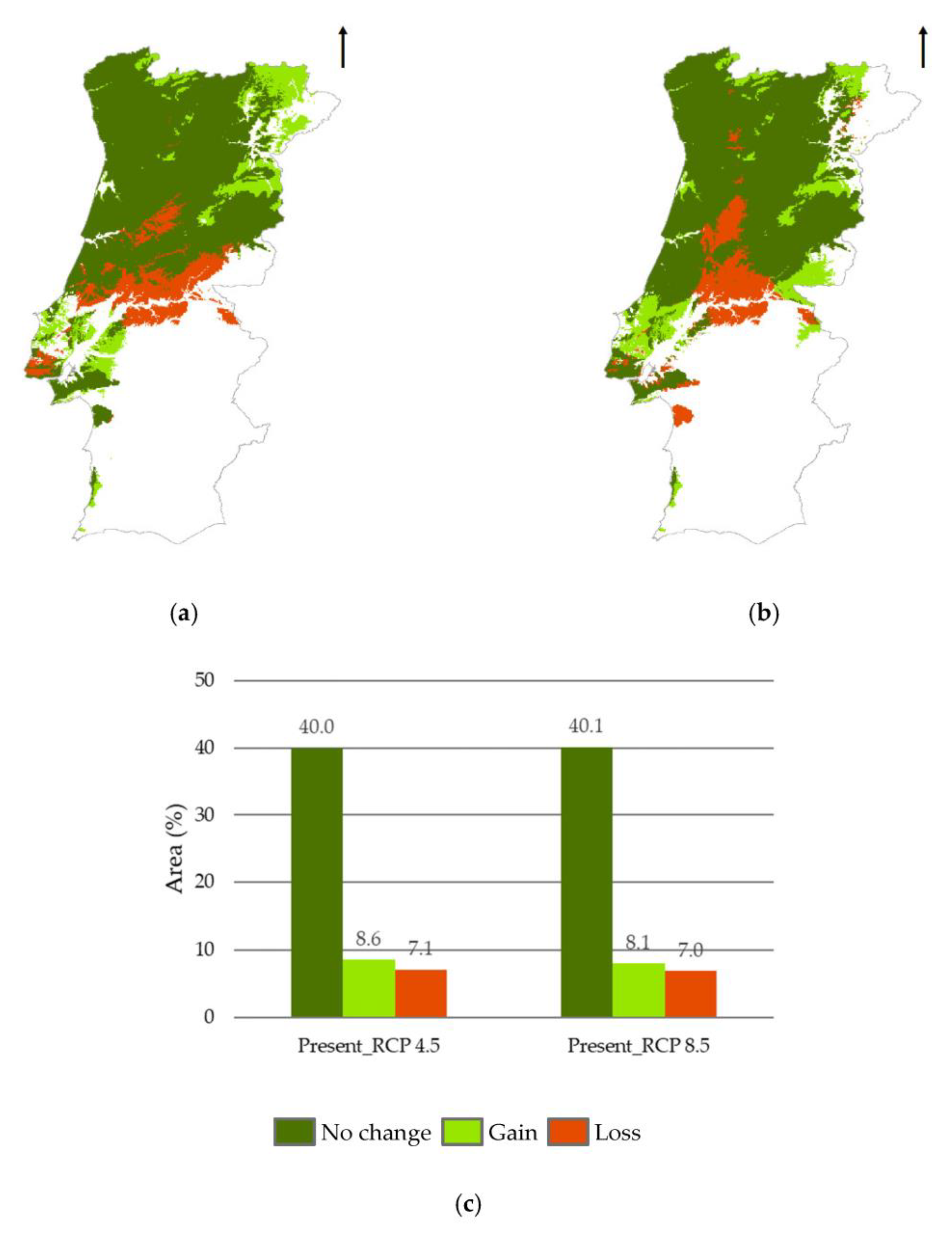
- van Vuuren, D.; Edmonds, J.; Kainuma, M.; Riahi, K.; Thomson, A.; Hibbard, K.; Hurtt, G.; Kram, T.; Krey, V.; La-marque, J.-F. The representative concentration pathways: An overview. Clim. Change 2011, 5–31. [Google Scholar] [CrossRef]
- Panagos, P. The European soil database. GEO Connex. 2006, 5, 32–33. [Google Scholar]
- Van Liedekerke, M.; Jones, A.; Panagos, P. ESDBv2 Raster Library—A Set of Rasters Derived from the European Soil Data-Base Distribution v2.0 (CD-ROM, EUR 19945 EN). European Commission and the European Soil Bureau Network. Available online: https://esdac.jrc.ec.europa.eu/content/european-soil-database-v2-raster-library-1kmx1km (accessed on 29 July 2018).
- IUSS Working Group WRB. World Reference Base for Soil Resources 2014, Update 2015 International soil Classifica-tion System for Naming Soils and Creating Legends for Soil Maps; World Soil: Rome, Italy, 2015. [Google Scholar]
- Phillips, S.J.; Anderson, R.P.; Dudík, M.; Schapire, R.E.; Blair, M.E. Opening the black box: An open-source release of Maxent. Ecography 2017, 40, 887–893. [Google Scholar] [CrossRef]
- Leroy, B.; Meynard, C.N.; Bellard, C.; Courchamp, F. virtualspecies, an R package to generate virtual species distributions. Ecography 2016, 39, 599–607. [Google Scholar] [CrossRef] [Green Version]
- Fielding, A.H.; Bell, J.F. A review of methods for the assessment of prediction errors in conservation presence/absence models. Environ. Conserv. 1997, 24, 38–49. [Google Scholar] [CrossRef]
- Radosavljevic, A.; Anderson, R.P. Making better MaxEnt models of species distributions: Complexity, overfitting and evaluation. J. Biogeogr. 2014, 41, 629–643. [Google Scholar] [CrossRef]
- Cohen, J. A coefficient of agreement for nominal scales. Educ. Psychol. Meas. 1960, 20, 37–46. [Google Scholar] [CrossRef]
- Landis, J.R.; Koch, G.G. The measurement of observer agreement for categorical data. Biometrics 1977, 33, 159–174. [Google Scholar] [CrossRef] [Green Version]
- Serra-Varela, M.J.; Grivet, D.; Vincenot, L.; Broennimann, O.; Gonzalo-Jiménez, J.; Zimmermann, N.E. Does phylogeographical structure relate to climatic niche divergence? A test using maritime pine (Pinus pinaster Ait.). Glob. Ecol. Biogeogr. 2015, 24, 1302–1313. [Google Scholar] [CrossRef]


| Study Area | Species Occurrences | ||||||||
|---|---|---|---|---|---|---|---|---|---|
| Symbol | Variable | Min | Max | Mean | Std | Min | Max | Mean | Std |
| BIO1 | Annual mean temperature (°C) | 5.9 | 17.6 | 15.0 | 1.8 | 8.6 | 17.6 | 14.3 | 1.5 |
| BIO2 | Mean diurnal range (°C) | 5.2 | 11.7 | 9.5 | 1.0 | 5.6 | 11.3 | 9.2 | 0.9 |
| BIO3 | Isothermality (%) | 31.0 | 50.0 | 39.8 | 2.7 | 31.0 | 50.0 | 39.8 | 2.7 |
| BIO4 | Temperature seasonality (%) | 2596.0 | 6118.0 | 4860.8 | 721.2 | 2788.0 | 6116.0 | 4778.2 | 747.2 |
| BIO5 | Max. temperature of the warmest month (°C) | 19.4 | 34.0 | 28.6 | 2.5 | 21.5 | 32.5 | 27.5 | 2.1 |
| BIO6 | Min. temperature of the coldest month (°C) | −2.9 | 9.2 | 5.0 | 2.3 | −1.5 | 8.8 | 4.5 | 2.0 |
| BIO7 | Temperature annual range (°C) | 12.2 | 29.3 | 23.5 | 2.9 | 13.4 | 28.8 | 23.0 | 2.9 |
| BIO8 | Mean temperature of the wettest quarter (°C) | 0.1 | 13.8 | 9.5 | 2.5 | 2.6 | 13.4 | 8.7 | 2.2 |
| BIO9 | Mean temperature of the driest quarter (°C) | 13.3 | 24.9 | 21.2 | 1.7 | 15.8 | 24.2 | 20.5 | 1.3 |
| BIO10 | Mean temperature of the warmest quarter (°C) | 13.3 | 25.0 | 21.4 | 1.8 | 15.9 | 24.3 | 20.6 | 1.4 |
| BIO11 | Mean temperature of the coldest quarter (°C) | 1.0 | 131.0 | 89.9 | 22.8 | 2.6 | 12.7 | 8.4 | 2.0 |
| BIO12 | Annual precipitation (mm) | 459.0 | 1798.0 | 844.8 | 270.4 | 475.0 | 1730.0 | 1022.2 | 209.4 |
| BIO13 | Precipitation of the wettest month (mm) | 64.0 | 272.0 | 122.1 | 38.5 | 65.0 | 270.0 | 148.4 | 31.0 |
| BIO14 | Precipitation of the driest month (mm) | 0.0 | 37.0 | 8.1 | 5.8 | 0.0 | 32.0 | 10.7 | 4.4 |
| BIO15 | Precipitation seasonality (%) | 39.0 | 72.0 | 56.3 | 5.4 | 39.0 | 71.0 | 54.7 | 3.4 |
| BIO16 | Precipitation of the wettest quarter (mm) | 180.0 | 719.0 | 346.9 | 102.8 | 180.0 | 711.0 | 415.3 | 80.8 |
| BIO17 | Precipitation of the driest quarter (mm) | 13.0 | 157.0 | 52.1 | 25.5 | 13.0 | 141.0 | 66.2 | 18.8 |
| BIO18 | Precipitation of the warmest quarter (mm) | 15.0 | 161.0 | 55.2 | 27.7 | 16.0 | 147.0 | 70.2 | 21.2 |
| BIO19 | Precipitation of the coldest quarter (mm) | 168.0 | 719.0 | 342.5 | 104.5 | 168.0 | 711.0 | 412.6 | 82.1 |
| E | Elevation (m) | 0.0 | 1959.0 | 322.7 | 263.7 | 2.0 | 1446.0 | 380.2 | 262.3 |
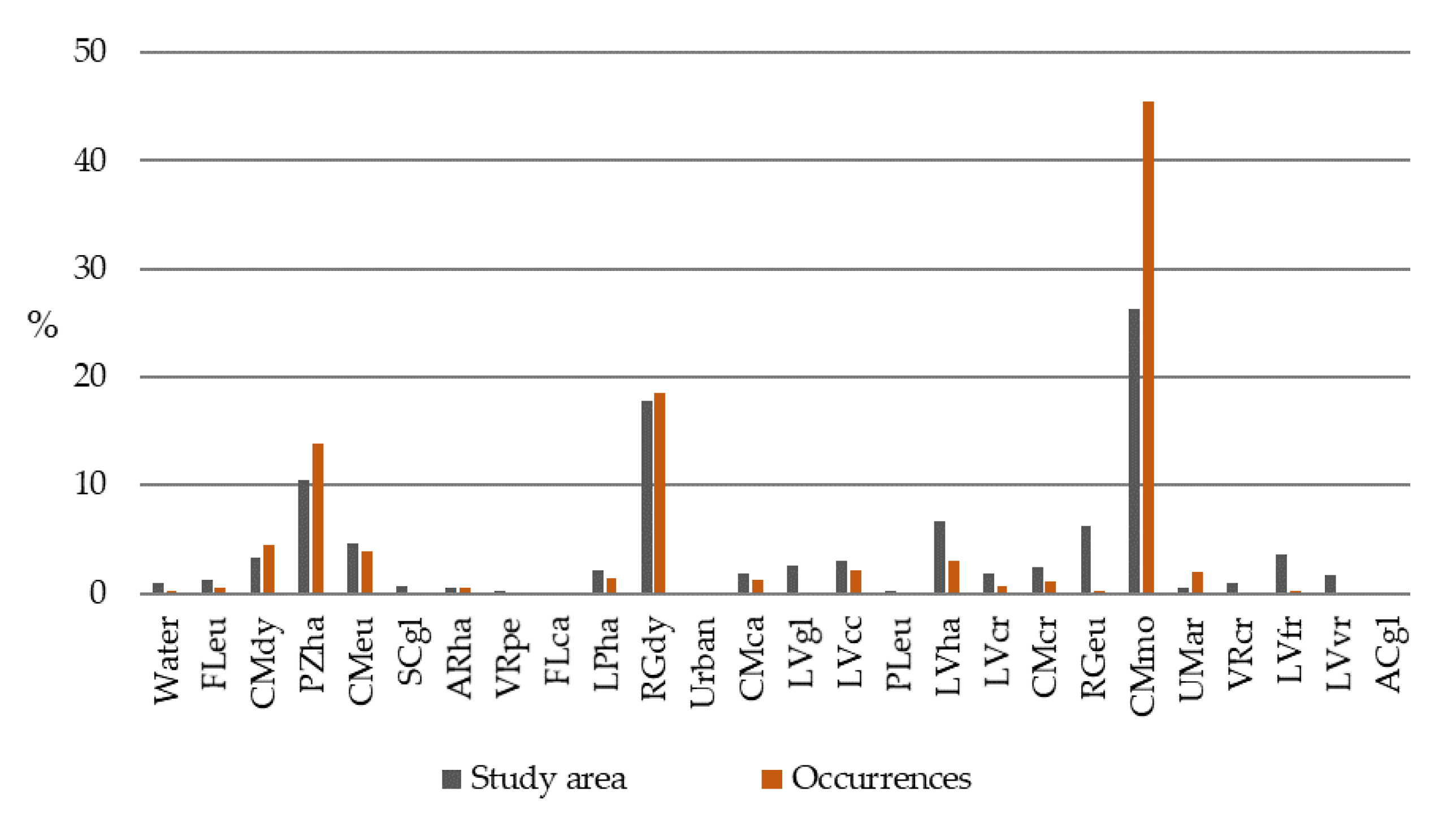
| Code | WRFBU | Group | Qualifier | Study Area (%) | Occurrences (%) |
|---|---|---|---|---|---|
| 2 | Water | - | - | 0.9 | 0.3 |
| 27 | FLeu | Fluvisol | Eutric | 1.2 | 0.6 |
| 29 | CMdy | Cambisol | Dystric | 3.3 | 4.6 |
| 30 | PZha | Podzol | Haplic | 10.5 | 13.8 |
| 35 | CMeu | Cambisol | Eutric | 4.6 | 4.0 |
| 54 | SCgl | Solonchak | Gleyic | 0.6 | 0.1 |
| 59 | ARha | Arenosol | Haplic | 0.6 | 0.5 |
| 65 | VRpe | Vertisol | Pellic | 0.2 | 0.0 |
| 67 | FLca | Fluvisol | Calcaric | 0.0 | 0.0 |
| 72 | LPha | Leptosol | Haplic | 2.1 | 1.4 |
| 74 | RGdy | Regosol | Dystric | 17.8 | 18.5 |
| 76 | Urban | - | - | 0.1 | 0.0 |
| 87 | CMca | Cambisol | Calcaric | 1.8 | 1.2 |
| 89 | LVgl | Luvisol | Gleyic | 2.6 | 0.0 |
| 90 | LVcc | Luvisol | Calcic | 3.1 | 2.1 |
| 91 | PLeu | Planosol | Eutric | 0.2 | 0.0 |
| 92 | LVha | Luvisol | Haplic | 6.6 | 3.1 |
| 107 | LVcr | Luvisol | Chromic | 1.8 | 0.7 |
| 108 | CMcr | Cambisol | Chromic | 2.4 | 1.1 |
| 109 | RGeu | Regosol | Eutric | 6.2 | 0.2 |
| 119 | CMmo | Cambisol | Mollic | 26.3 | 45.5 |
| 124 | UMar | Umbrisol | Arenic | 0.5 | 2.0 |
| 125 | VRcr | Vertisol | Chromic | 1.0 | 0.1 |
| 127 | LVfr | Luvisol | Ferric | 3.7 | 0.2 |
| 129 | LVvr | Luvisol | Fluvic | 1.6 | 0.0 |
| 130 | ACgl | Acrisol | Gleyic | 0.0 | 0.0 |
| Temperature Limits (°C) | Temperature Range (°C) | Precipitation (mm) | Elevation (m) | Soil |
|---|---|---|---|---|
| BIO5 < 29.8 BIO6 > 2.6 | BIO7 ≤ 25.1 | BIO12 > 821 | E < 731 | Soils different of Limestone (LVcc, CMca, and FLca) |
| Kappa Value | Interpretation |
|---|---|
| Below 0.00 | Poor |
| 0.00–0.20 | Slight |
| 0.21–0.40 | Fair |
| 0.41–0.60 | Moderate |
| 0.61–0.80 | Substantial |
| 0.81–1.00 | Almost perfect |
| Procedure | Variables | AUC | 10th Percentile * |
|---|---|---|---|
| MaxEnt (7 var) | BIO4, BIO10, BIO12, BIO13, BIO18, E, WRBFU | 0.74 | 0.39 |
| Virtualspecies (VS 6 var) | BIO3, BIO4, BIO5, BIO8, BIO15, WRBFU | 0.73 | 0.39 |
| Envelope variables (6 var) | BIO5, BIO6, BIO7, BIO12, E, WRBFU | 0.74 | 0.40 |
| MaxEnt 7 var | VS 6 var | Envelope 6 var | ||||||||||||
|---|---|---|---|---|---|---|---|---|---|---|---|---|---|---|
| Var | PC | PI | TGw | TGo | Var | PC | PI | TGw | TGo | Var | PC | PI | TGw | TGo |
| BIO12 | 52.49 | 2.53 | 0.37 | 0.27 | BIO5 | 34.80 | 15.57 | 0.32 | 0.13 | BIO12 | 72.91 | 59.93 | 0.32 | 0.27 |
| BIO13 | 18.54 | 29.21 | 0.37 | 0.27 | BIO15 | 31.30 | 18.38 | 0.33 | 0.13 | WRBFU | 15.22 | 8.73 | 0.34 | 0.21 |
| WRBFU | 14.50 | 12.43 | 0.34 | 0.21 | WRBFU | 21.48 | 13.47 | 0.31 | 0.21 | BIO5 | 4.35 | 8.34 | 0.36 | 0.12 |
| BIO10 | 5.35 | 13.86 | 0.36 | 0.15 | BIO4 | 6.63 | 28.29 | 0.33 | 0.04 | BIO6 | 3.21 | 12.17 | 0.36 | 0.07 |
| BIO18 | 4.59 | 20.63 | 0.36 | 0.22 | BIO8 | 3.90 | 16.87 | 0.34 | 0.09 | BIO7 | 2.58 | 4.77 | 0.36 | 0.06 |
| BIO4 | 3.18 | 14.98 | 0.36 | 0.04 | BIO3 | 1.89 | 7.42 | 0.34 | 0.02 | E | 1.73 | 6.06 | 0.36 | 0.06 |
| E | 1.35 | 6.36 | 0.37 | 0.06 | ||||||||||
| Scenario | Kappa Index | Interpretation |
|---|---|---|
| Present | 0.32 | Fair |
| Future 2070–RCP 4.5 | 0.26 | Fair |
| Future 2070–RCP 8.5 | 0.24 | Fair |
Disclaimer/Publisher’s Note: The statements, opinions and data contained in all publications are solely those of the individual author(s) and contributor(s) and not of MDPI and/or the editor(s). MDPI and/or the editor(s) disclaim responsibility for any injury to people or property resulting from any ideas, methods, instructions or products referred to in the content. |
© 2023 by the authors. Licensee MDPI, Basel, Switzerland. This article is an open access article distributed under the terms and conditions of the Creative Commons Attribution (CC BY) license (https://creativecommons.org/licenses/by/4.0/).
Share and Cite
Alegria, C.; Almeida, A.M.; Roque, N.; Fernandez, P.; Ribeiro, M.M. Species Distribution Modelling under Climate Change Scenarios for Maritime Pine (Pinus pinaster Aiton) in Portugal. Forests 2023, 14, 591. https://doi.org/10.3390/f14030591
Alegria C, Almeida AM, Roque N, Fernandez P, Ribeiro MM. Species Distribution Modelling under Climate Change Scenarios for Maritime Pine (Pinus pinaster Aiton) in Portugal. Forests. 2023; 14(3):591. https://doi.org/10.3390/f14030591
Chicago/Turabian StyleAlegria, Cristina, Alice M. Almeida, Natália Roque, Paulo Fernandez, and Maria Margarida Ribeiro. 2023. "Species Distribution Modelling under Climate Change Scenarios for Maritime Pine (Pinus pinaster Aiton) in Portugal" Forests 14, no. 3: 591. https://doi.org/10.3390/f14030591