Article

Predicting the Habitat Suitability for Angelica gigas Medicinal Herb Using an Ensemble Species Distribution Model

1
Forest Ecology Division, National Institute of Forest Science, Seoul 02445, Republic of Korea
2
Forest Medicinal Resources Research Center, National Institute of Forest Science, Yeongju 36040, Republic of Korea
*
Authors to whom correspondence should be addressed.
Forests 2023, 14(3), 592; https://doi.org/10.3390/f14030592
Submission received: 27 February 2023 / Revised: 14 March 2023 / Accepted: 15 March 2023 / Published: 16 March 2023
(This article belongs to the Section Forest Ecology and Management)

Abstract

:
The distribution shift of forest species due to the fact of climate change may negatively affect ecosystem services including the production of medicinal resources. Climate change impact assessments of habitat range changes are essential to sustainably manage forest resources. A change in the habitat suitability due to the fact of climate change was predicted for Angelica gigas, which has high economic value among forest medicinal resources in South Korea. The habitat suitability was predicted by an ensemble species distribution model that combined the results of nine single algorithm models using the committee averaging method. A total 168 occurrence data and 10 environmental variables were used for the single algorithm models. The area under the receiver operation characteristic curve (AUC) and true skill statistic (TSS) were applied to evaluate the models’ performance, and the contribution of the environmental variables was calculated as an important value for each single algorithm model. Climate change scenarios were projected to predict future habitat suitability. The future suitable habitat for A. gigas was gradually reduced to the high mountain regions of the eastern part of South Korea regardless of the climate change scenarios. The main environmental variable was the annual mean temperature, and the rise in temperature due to the fact of climate change was found to have a negative effect on the habitat suitability for A. gigas. The decline in the habitat suitability for A. gigas, a major forest medicinal resource, is expected to result in the reduction in its production. Therefore, it is required to establish adaptation measures to mitigate the negative impact of this decrease, such as protecting the natural habitats of A. gigas.

1. Introduction

The climate is a critical factor that impacts the physiological response and life cycle of forest organisms, and climate change causes habitat range shifts by affecting growth and reproduction [1]. Increases in the elevation or poleward shifts of habitat ranges observed in forest ecosystems clearly demonstrate the impact of climate change on species distribution [2,3,4]. Consequently, the change in species distribution may exert not only a significant influence on the structure of forest ecosystems, including biodiversity, but also an adverse impact on the provision of ecosystem services [5]. Therefore, predicting changes in species distribution under climate change can be considered a prerequisite for the sustainable management of ecosystem services and the mitigation of adverse impacts [6].
The species distribution model (SDM) involves a series of data processing and an algorithm that predicts the occurrence probability or habitat suitability through the assumption of the relationship between species occurrence and circumstantial environmental variables. The SDM is widely used as a quantitative assessment tool of the impact of climate change [6,7]. However, since predicting habitat suitability includes multiple uncertainties and errors according to the traits of the species, the algorithm, spatial distribution of the occurrence data, sampling method, and collinearity among the explanatory variables, caution in terms of these uncertainties must be taken before interpreting the model results [8,9,10]. As a practical example, previous research on the future habitat suitability for subalpine evergreen conifers in South Korea showed different results according to the occurrence data, model algorithm, environmental variables, and climate change scenarios [11,12]. Therefore, a methodology that can increase the reliability and reduce the uncertainty of the SDM’s results is required [13].
The ensemble approach refers to a statistical agreement method for reducing the model uncertainties caused by the model algorithm and parameters or the climate uncertainties due to the projected climate conditions and, generally, increases the predictive ability compared to a single algorithm model [14,15]. In addition, a consistent agreement can be derived through averaging (e.g., the multimodel inference, arithmetic average, and weighted average), and it is widely applied in decision making for climate change adaptation [16,17]. In South Korea, research that applies the ensemble approach is actively conducted; however, the majority of this research has studied the model uncertainty [12,18,19], and there has been a lack of its application to multiple climate change scenarios for reducing climate uncertainty [20,21]. Wenger et al. [22] documented that in future species distribution prediction, the climate uncertainty was greater than the model uncertainty, and there is an increasing need for an ensemble approach that considers multiple climate conditions during climate change impact assessment [23,24].
Angelica gigas Nakai is endemic to East Asia and mostly lives in the valleys of mountainous area in the Korean Peninsula at an elevation of ≥700 m [25,26]. It is a highly valuable medicinal plant that is traditionally used in Korean herbal medicine, and it is currently produced though local harvesting and cultivation [27]. Although A. gigas production heavily relies on cultivation, harvesting remains an important production method. The production of A. gigas is closely related to the climate conditions during the growing period [28,29]. Exposure to high temperatures at the onset of growth not only reduces the development of the aboveground and underground parts of A. gigas but also decreases the survival rate [30]. In addition, previous research that compared the growth of A. gigas for each climate zone and altitude showed that a higher temperature led to the reduced growth of the aboveground and underground parts [31,32]. Poor growth and an increase in mortality are closely related to the species distribution [33]; therefore, temperature increases due to the fact of climate change could induce changes in the distribution of A. gigas; however, there is a lack of studies on the change in habitat suitability for A. gigas [34].
This study aimed to assess the impact of climate change on the distribution of A. gigas and identify a suitable habitat for A. gigas. In detail, this study was purposed to (1) develop an optimal ensemble model for examining habitat suitability for A. gigas, (2) determine the relative importance of each environmental variable in predicting the habitat suitability, and (3) identify the change over time in the suitable habitat. In addition, this study used multiple climate change scenarios that can reduce climate uncertainties to increase the reliability of the predicted results.

2. Materials and Methods

2.1. Collection of Species Occurrence Data

Occurrence data for A. gigas in South Korea were obtained from the 7th National Forest Inventory (NFI, 2016–2020), the monitoring data on endangered subalpine evergreen conifers of the Korea Forest Service (ESCM, 2017–2018), the 4th National Natural Environment Survey of the National Institute of Ecology (NNES, 2014–2018) [35], the Global Biodiversity Information Facility (GBIF, 1957–2010) [36], and Park (2018) [37] (Table 1). However, if there were occurrences in a cultivated area, they were removed from the occurrence data. This is because the distribution of cultivated populations is influenced not only by environmental variables but also artificial management practices such as fertilization, making it difficult to distinguish the effects of these factors on the distribution. As A. gigas is cultivated in open fields rather than forests, where the natural population occurs [25,27], the location of each occurrence was carefully verified using Google satellite imagery, and the occurrences in cultivated areas were excluded from the analysis. To reduce the spatial autocorrelation in the locations of A. gigas occurrence, the occurrence data were thinned using a distance of 1 km. Finally, the occurrence data from 168 out of 285 locations were used to construct the species distribution model (Figure 1).

2.2. Selection of Environmental Variables

A total of 19 bioclimate variables provided by WorldClim version 2.1 were used for the baseline climate (1970–2000) for constructing the species distribution model [38]. The period from 1970 to 2000 was selected because it corresponds to a notable shift in climate regimes that has been evidenced by several studies [39,40]. These studies indicate that changes in both precipitation and temperature began in the mid-1970s, underscoring the importance of this period in understanding the impact of climate change on A. gigas distribution. For the future climate, the 19 bioclimate variables of the SSP245 and SSP585 scenarios predicted by ACCESS-ESM1.5 [41], CNRM-ESM2-1 [42], HadGEM3-GC31-LL [43], IPSL-CM6A-LR [44], and MIROC6 [45] among the global climate models (GCMs) of CMIP6 were used. The time ranges of the future climate were 2021–2040, 2041–2060, 2061–2080, and 2081–2100. The mean value of the climate variable of each time range was used in the prediction of future habitat suitability and are indicated in the results as 2030, 2050, 2070, and 2090.
Global Multi-Resolution Terrain Elevation Data (GMTED2010) with a spatial resolution of approximately 1 km2 (30 arc-second) were used to determine the topographical variables of the altitude, slope, and aspect [46]. In addition, the occurrence characteristics of A. gigas that mainly grows near mountain valleys were considered, and the topographic wetness index (TWI) with a 30 arc-second scale, created by the Korea Institute of Geoscience and Mineral Resources (KIGAM), was added [47]. TWI represents the soil moisture variation according to the slope and aspect, and a greater value implies a greater topographical moisture content retention capacity.
Finally, as soil variables, the cation exchange capacity (CEC), which has been found to be closely related with the growth of A. gigas [26,28], and bulk density (BOD), which is related to the soil texture and soil porosity, were used among the soil data provided by SoilGrids 2.0 [48]. The collinearity that exists between the explanatory variables of climate, topography, and soil increases the uncertainty of the species distribution model’s results [10], and Spearman’s rank correlation analysis was performed to remove variables with a correlation coefficient of >0.7 from the analysis [49]. Altitude showed a strong positive correlation (rs = 0.78) with the annual mean temperature (BIO1); therefore, it was eliminated from the final explanatory variable, and 10 environmental variables were selected, as follows, for use in the development of the species distribution model (Figure S1; Table 2). All environmental variables had a spatial resolution of approximately 1 km2 (30 arc-second). The same topographical and soil variables were used in both the baseline and future projections, as these variables are not expected to change significantly over short time frames.

2.3. Development and Evaluation of the Species Distribution Model

A total of nine algorithms, including artificial neural network (ANN), classification tree analysis (CTA), generalized additive model (GAM), generalized boosting regression model (GBM), generalized linear model (GLM), multiple adaptive regression splines (MARS), maximum entropy (MAXENT), random forest (RF), and surface range envelop (SRE), were used to create the species distribution model [13,50]. Some algorithms require not only presence data but also absence data, for which this research randomly extracted 1000 pseudo-absence data 10 times to generate 10 presence–absence datasets. The training and validation data were distinguished from each dataset at a ratio of 7:3 and were used in the model creation (70%) and model accuracy evaluation (30%), respectively. The single algorithm model was created 10 times for each dataset using the environmental variables, and the contribution of the environmental variables was determined for each model.
Cross-validation was performed five times to assess the accuracy of the single algorithm models. For this purpose, the validation data for each dataset were used to determine the area under the receiver operation characteristic curve (AUC) and the true skill statistic (TSS). The AUC was produced using the true positive rate (i.e., sensitivity) and the false positive rate from the classification table [51]. The sensitivity is the fraction of the actual presence that was correctly predicted as presence, while the false positive rate presents the extent of the false presence among the actual absence. The TSS was determined using the sensitivity and the true negative rate (i.e., specificity), which represents the extent of the prediction as absence among the actual absence, and the calculation of the TSS was as follow [52].
True skill statistic (TSS) = Sensitivity + Specificity − 1
The prediction performance can be considered good when both the AUC and TSS are close to 1. In this study, the model results were determined to be reliable when the AUC was ≥0.7 and the TSS was ≥0.6 [52,53].

2.4. Prediction of Ensemble Model

Among the single algorithm models, those with a TSS index of ≥0.6 were selected to create an ensemble model with the committee averaging (CA) method [54]. CA is a method of cumulatively adding the occurrence probabilities after the binary conversion of the occurrence probability into 0 and 1 from the single algorithm model and dividing the sum into the total number of models [50]. The final product of the CA ensemble model is not a continuous variable; therefore, it has the advantages of being intuitive and easy for comparison [55]. To reduce the climate uncertainty, two climate change scenarios (SSP245 and SSP585) from five GCMs were projected to determine the mean value of each time range’s occurrence probability [21]. To distinguish the suitable habitat, the occurrence probability at the intersection of the sensitivity and specificity at which the TSS is maximized was designated as a threshold value for each climate scenario, and binary conversion was performed. The suitable habitat areas for each time range were determined on the binarized map, and the amount of reduction regarding the habitable area in 1970–2000 is presented in rates (%). In addition, the mean altitudes of the locations distinguished as having the presence of A. gigas were calculated to review the tendency of the change in altitude according to the climate change scenario. All analyses were performed using the Biomod2 package [50] in the R program [56].

3. Results

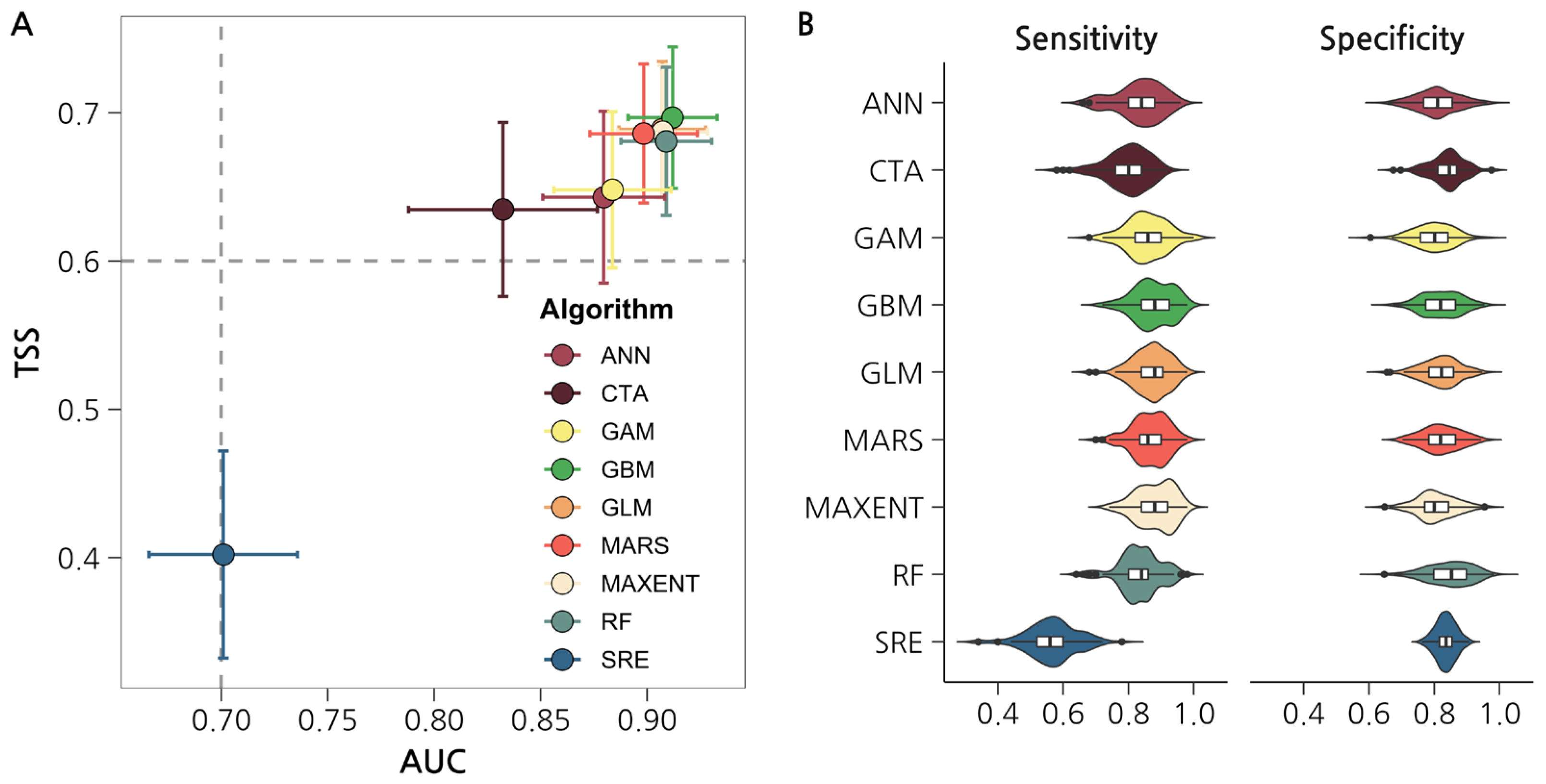
3.1. Performance of the Single Algorithm and Ensemble Model

All algorithms used in this study, excluding SRE, suitably predicted the presence of A. gigas (Figure 2A). The AUC and TSS mean values of all single algorithm models were 0.87 ± 0.07 and 0.64 ± 0.10, respectively, and the GBM showed the highest AUC and TSS values among the single algorithm models (AUC = 0.91 ± 0.02; TSS = 0.70 ± 0.05), followed by the GLM, MARS, MAXENT, and RF. The lowest prediction performance was that of SRE (AUC = 0.70 ± 0.03; TSS = 0.40 ± 0.07).
In the ensemble model that was created with the models that had a TSS of ≥0.6 among the single algorithm models, 98 GLM models were included and accounted for the greatest number of models, followed by 97 GBM and MARS models, 96 MAXENT models, 94 RF models, 83 GAM models, 78 ANN models, and 74 CTA models, which contributed to the ensemble model. In contrast, all SRE models were excluded from the ensemble model. The AUC and TSS of the ensemble model were 0.96 and 0.78, respectively, and showed a superior prediction ability compared to the single algorithm models. The sensitivity of each single algorithm model was highest in the MAXENT (0.88 ± 0.06), and the specificity was 0.85 ± 0.07 in the RF, which was higher than that in the other algorithm models (Figure 2B). The specificity of the SRE was lower than the sensitivity, and the overall prediction ability was low.

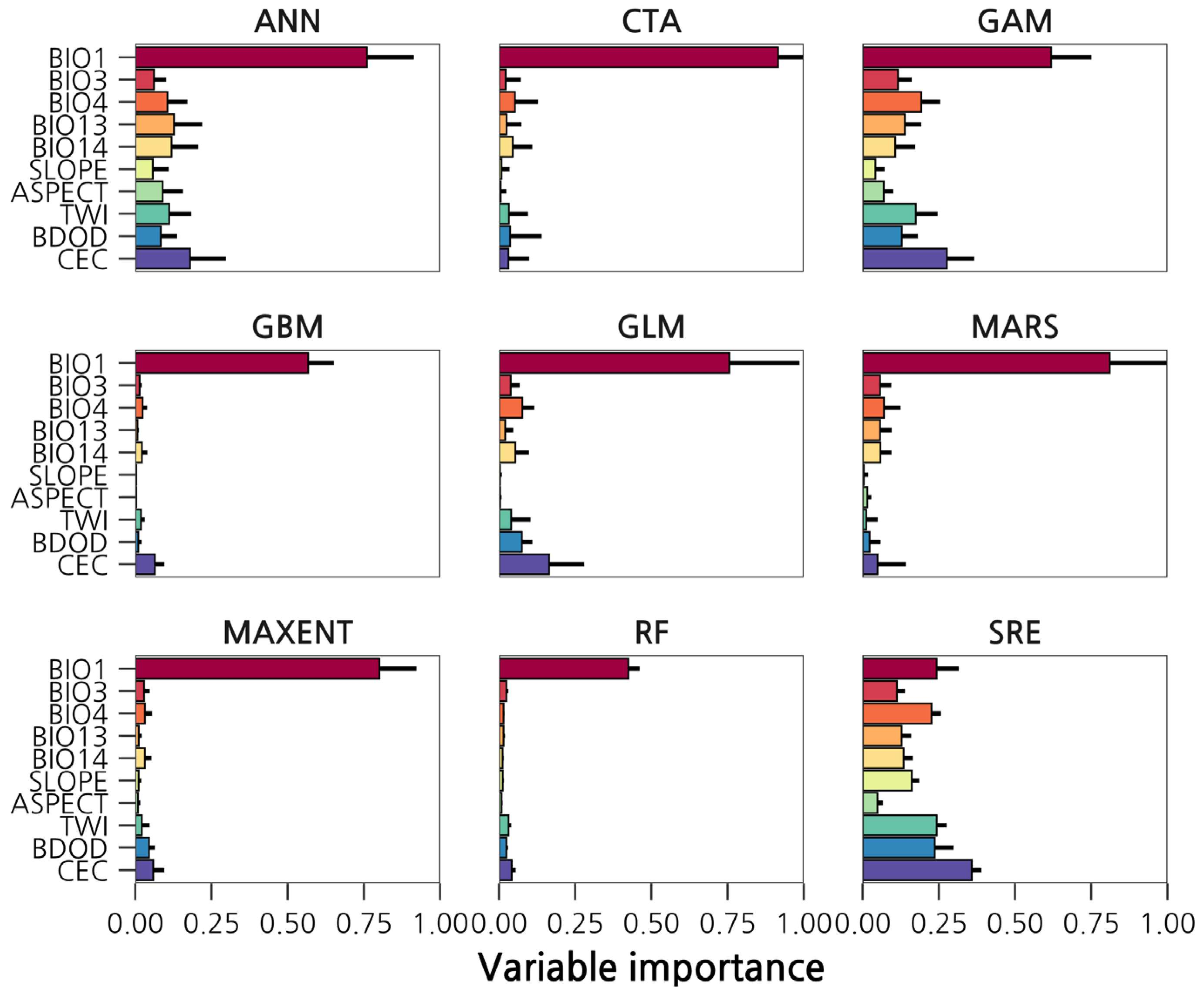
3.2. Habitat Suitability and Environmental Variable Contribution

The suitable habitat area for A. gigas predicted by the ensemble model under the baseline climate conditions (1970–2000) was 25,130 km2, and the habitat suitability was high in the eastern regions and the high-altitude areas of some mountains in the southern regions of South Korea (Figure 3A). The single algorithm models showed similar spatial tendencies to the ensemble model; however, there was a difference in the habitat suitability (Figure S2). Among the nine algorithms, the MAXENT and RF predicted a low probability of the habitat being suitable, and the SRE showed a relatively higher habitat suitability than the other algorithms (Figure 3B).
The environmental variable that related most to the occurrence of A. gigas was the annual mean temperature (BIO1) (Figure 4). The variable importance of the annual mean temperature identified from 900 single algorithm models was 0.66 ± 0.45, and it best described the occurrence of A. gigas among the environmental variables used in the species distribution model. The variable importance of the annual mean temperature was the highest at an average of 0.92 ± 0.12 in the CTA algorithm model, and it showed the lowest value (0.24 ± 0.07) in the SRE algorithm model. After the annual mean temperature, the importance value of the CEC was high, with the total model average being 0.14, and it had a greater impact on the occurrence of A. gigas than the topographical variables. Among the topographical variables, the TWI showed a greater contribution than the slope and aspect.

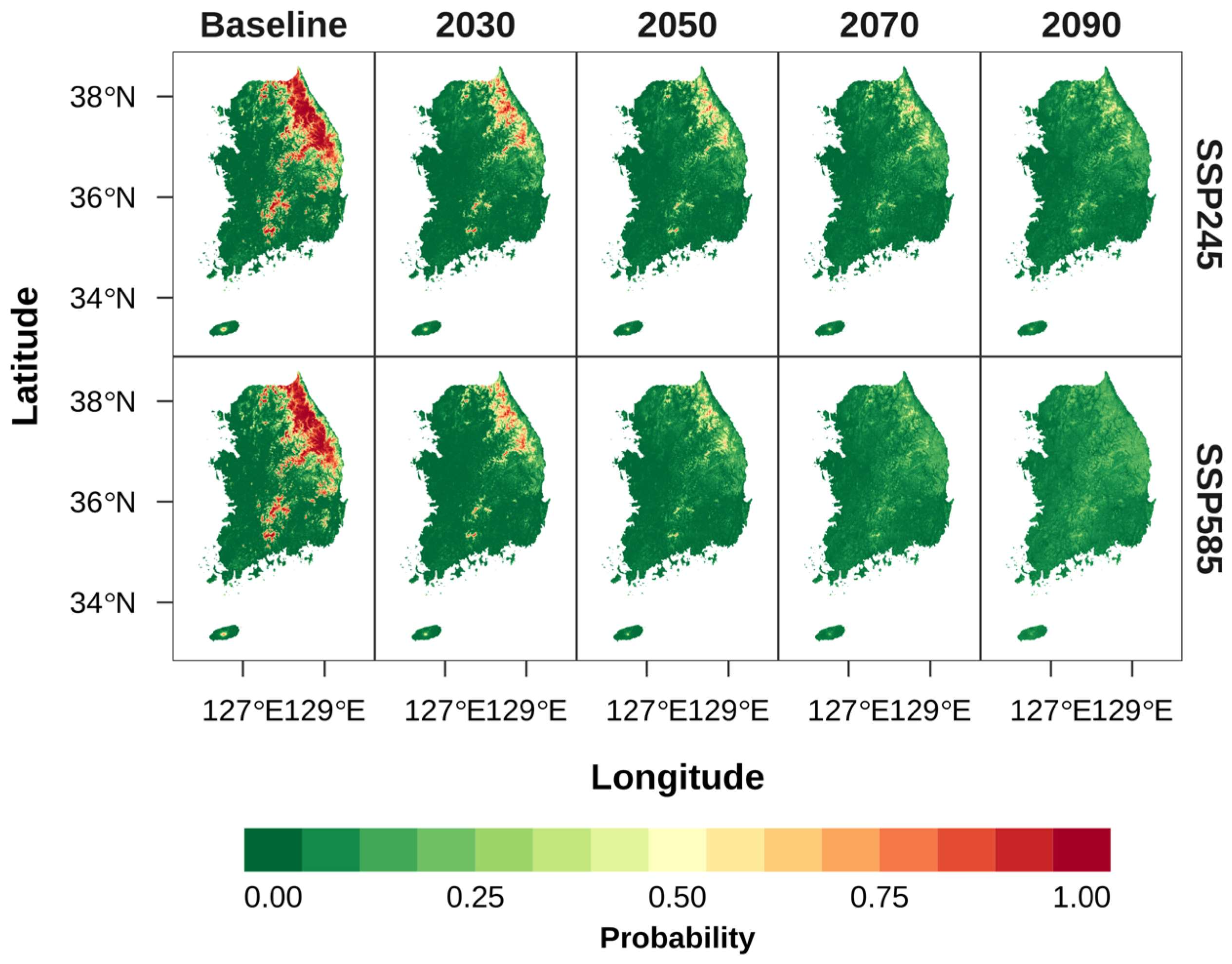
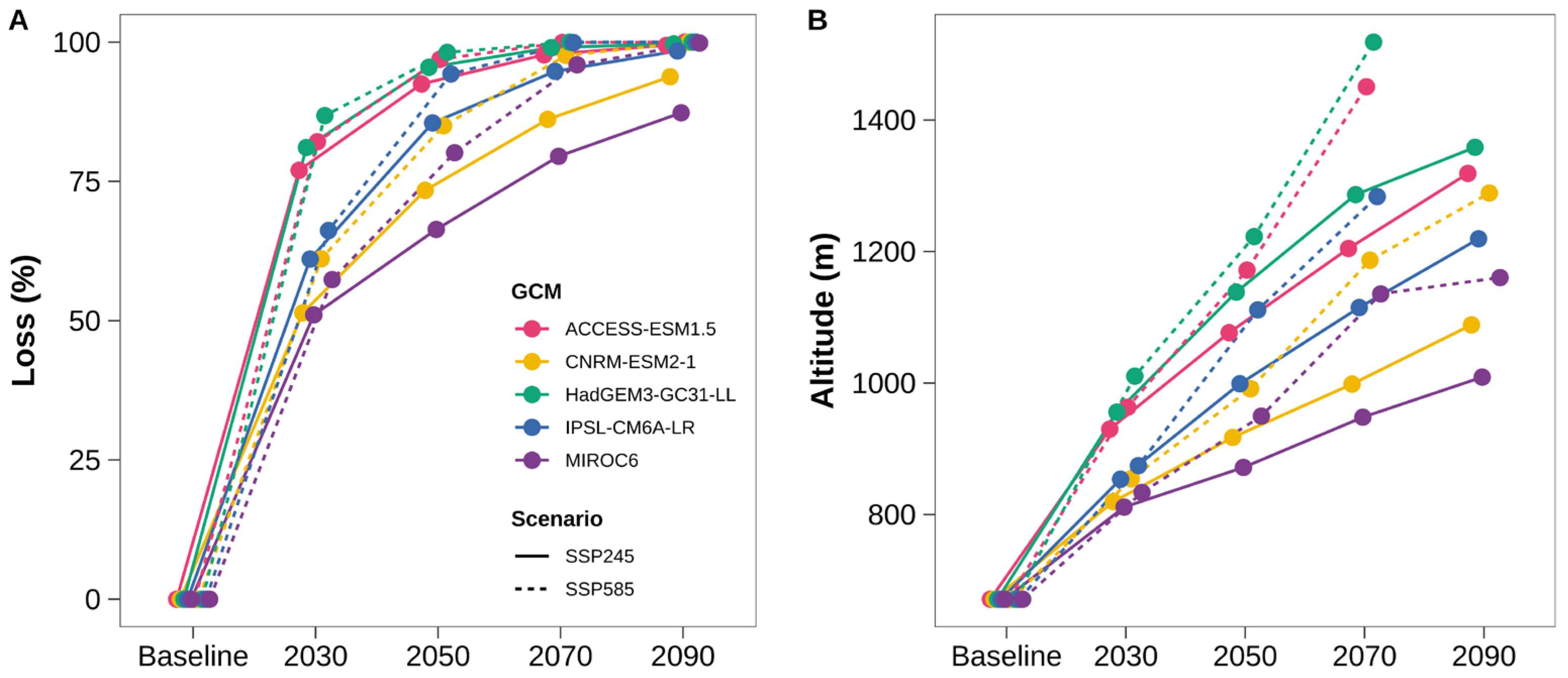
3.3. Future Changes in Suitable Habitat

The habitat suitability predicted by reflecting five GCMs and two SSP combinations with the climate change scenarios decreased in the low-altitude regions, and the suitable habitat areas gradually narrowed down to the high-altitude regions, such as mountainous areas (Figure 5). The mean habitat suitability was lower in the SSP585 scenario than the SSP245 scenario for all time ranges. The mean suitable habitat areas of A. gigas in 2030 were 8967 ± 3170 km2 for SSP245 and 7358 ± 2931 km2 for SSP585, which were reductions of 64 ± 13% and 71 ± 12%, respectively, compared to the habitat areas under the baseline climate conditions (Table 3; Figure 6A). In approximately 2090, A. gigas occurrence was predicted only from a mean area of 9 km2 in SSP585 and of 1074 km2 in SSP245. The greatest decrease in the suitable habitat area was observed in HadGEM3-GC31-LL, followed by that in ACCESS-ESM1.5, IPSL-CM6A-LR, CNRM-ESM2-1, and MIROC6. In the case of HadGEM3-GC31-LL, the decreases in the area in the SSP245 scenario were 81.1% in 2030 and 99.7% in 2090, and the reductions were 86.8% in 2030 and 100% in 2090 in the SSP585 scenario. In contrast, for MIROC6, with the lowest predicted decrease in the area, the SSP245 scenario showed decreases of 51.0% in 2030 and 87.3% in 2090. The reductions were 57.4% and 99.8% in 2030 and 2090, respectively, in the SSP585 scenario. The mean altitude of suitable habitat was 671 m under the baseline climate conditions; however, according to SSP585, it tended to increase from 907 m in 2030 to 1089 m in 2050, 1315 m in 2070, and 1225 m in 2090, and a suitable habitat for A. gigas gradually reduced to mountainous areas with a high altitude (Figure 6B). The annual mean temperature is expected to increase from 11.3 °C in 1970–2000 to 13.1 °C for SSP245 and 13.3 °C for SSP585 by 2030 (Figure S3). By 2090, the annual mean temperature is expected to rise to 15.0 °C for SSP245 and 17.5 °C for SSP585.

4. Discussion

An ensemble species distribution model was used to predict the future habitat suitability for A. gigas under multiple climate change scenarios. The AUC and TSS values of the ensemble model created with the committee averaging method were 0.96 and 0.78, respectively, and showed a relatively higher prediction ability than the single algorithm models and contributed to reducing the model uncertainty of the prediction by merging the different results for each algorithm into one [14,15]. Therefore, the results of this study that predicted the distribution of A. gigas using the ensemble model are applicable as preliminary data for selecting suitable habitats for A. gigas. However, the ensemble model evaluation used validation data from an identical dataset; hence, the ensemble model’s performance may deteriorate when the model is transferred into the independent temporal and spatial ranges from the training data [57]. Further, in the case of optimizing the model through mediation of the parameters, the performance of the single algorithm model could be higher than that of the ensemble model, which used the defaults, for which the use of an ensemble model requires the accurate assessment of the ensemble model performance through additional procedures, such as the null model or external validation aside from internal validation [58,59]. Therefore, in future research, it seems reasonable to validate the model using spatial blocking or independent validation data [58]. In addition, preventing overfitting of the single algorithm model through mediation of the model parameters could support the improvement of the accuracy and overall transfer capacity of the ensemble model.
Among the nine algorithms used in this research, the GBM showed the highest accuracy in predicting the occurrence of A. gigas. This high prediction ability of the GBM can be identified in several previous studies that compared the model algorithms [60,61], and a study in South Korea on subalpine evergreen conifers demonstrated the high predictive performance of the GBM along with the RF [12]. The GBM not only has the strengths of the boosting technique, such as machine learning and regression tree, but also the advantage of being able to consider the nonlinear relationship and interaction between explanatory variables, which is not possible in regression analysis algorithms, such as GLM or GAM [62]. The GBM is sensitive to the number of occurrence data and is known to have a higher accuracy compared to other algorithms in the case of having a significant number of occurrence data (≥100) [63]. Therefore, if the results from the GBM algorithm model are given preference along with the ensemble model when selecting an appropriate habitat for A. gigas, this can increase the reliability of decision making.
The other algorithms, excluding SRE, were also found to have a suitable prediction ability based on the AUC and TSS, and they were referenced for the prediction of suitable habitats for A. gigas. This could contribute to the complementation of erased or missing ecological information from the ensemble model by preserving the ecological relationship assumed by each algorithm. On the contrary, the TSS value of the SRE algorithm was low, and some research in South Korea has verified the low accuracy of the SRE compared to other algorithms; therefore, the use of the SRE algorithm appears to require caution during the creation of the ensemble model [18,21].
The natural habitats of A. gigas are found in the valleys or gentle slopes of high mountains, and these habitats form on altitudes of ≥700 m in the eastern regions and ≥1000 m in the southern regions of South Korea [25,26]. In this study, it was observed that the suitable habitats for A. gigas exist at altitudes above the mean value of 671 m, as determined by the baseline conditions. This is attributed to the intrinsic correlation between altitude and temperature, wherein altitude indirectly affects the growth, reproduction, and distribution of A. gigas by influencing the prevailing environmental conditions, including temperature [31,32]. Temperature, especially during summer, significantly impacts the growth of A. gigas [34,37]. Furthermore, this study discovered that the mean temperature during the warmest quarter (BIO10) of the baseline climate conditions (1970–2000) at the location of the occurrence data was 19.3 °C, which closely aligns with the optimal growth temperature in July–August of approximately 20 °C reported in earlier research [27,37]. Based on the given scenario, it is highly probable that the impact of temperature on growth will intensify alongside the rise in the average annual temperature. Previous research shows that as the altitude of the cultivation site increases and the climate becomes cooler, the survival rate of transplanted A. gigas increases, and there is also a noticeable increase in the underground biomass [31,64]. In contrast, high temperatures adversely affect A. gigas growth, and the biomass of the aboveground and underground parts decrease when the temperature increases to above 20–25 °C, which is the optimal growing temperature for A. gigas [27,28]. Jeong et al. [30] showed that the extent of the reduction of the aboveground and underground biomasses increased as the temperature increased with regard to the optimal growing temperature. The highly significant effect of the annual mean temperature (BIO1) on the prediction of the habitat suitability for A. gigas may have reflected the changes in the growth characteristics according to the optimal growing temperature.
Temperature is not only related to vegetative growth but also to reproductive growth and regeneration. A. gigas is a long-day plant, which forms the flower stalk when the photoperiod elongates, and the rate of flower stalk formation is highest at 20 °C regardless of the photoperiod conditions, followed by that at 15 °C and 25 °C [27]. Meanwhile, Cho and Kim [65] studied the A. gigas germination rate, and stated that the rate decreased from 62.7% to 22.3% when the temperature increased from 20 °C to 30 °C. Choi and Yun [66] also reported that the germination rate was the highest at the optimal temperature for growth, and that a temperature increase from that level decreased the germination rate. Overall, an increase in temperature appears to impede the dispersion of A. gigas by negatively affecting its growth and regeneration.
A. gigas naturally inhabits regions with high moisture conditions such as valleys [25]; however, the results of this study showed that the TWI or aspect had a lower variable importance than that of the other climate variables. Interestingly, a study conducted on Mt. Hallasan, Jeju Island, found that the height of A. gigas on the north-facing slope was higher than that on the south-facing slope [67]. Additionally, Park et al. [28] reported the high growth of the underground parts at a high air humidity. These findings suggest that moisture conditions may play a role in the growth and distribution of A. gigas, but their impact may be more complex than previously thought. One possible explanation of the low variable importance of the TWI and aspect in this study is that the spatial resolution of these variables may be too coarse to adequately capture the microscale soil moisture variations. Therefore, further research is needed to understand the growth and distribution of A. gigas in relation to the moisture conditions.
The CEC was used as the explanatory variable for the model in this study to indicate the content of exchangeable cations, and the results showed that CEC had the strongest relationship to the distribution of A. gigas, after the annual mean temperature. This result agrees with the results of a study that showed that A. gigas mainly inhabits soils with high organic matter content, total nitrogen content, CEC, and exchangeable cations content [25]. According to Park et al. [28], the biomass of A. gigas’s roots increased with a higher CEC, and the Ca+, Mg2+, and Na+ contents were positively correlated to root growth [26]. Chang and Choi [68] inferred that exchangeable cations or CEC positively impacted the growth of A. gigas, since potassium fertilizer increased the growth of its aboveground and underground parts. In addition, vigorous root development could be considered to impact the spatial distribution of individual A. gigas indirectly and directly by contributing to increasing the survival rate and resistance to physical disturbances that occur frequently in valley and boulder areas (as the main habitats).
In the ensemble model, the predicted suitable habitat area for A. gigas tended to gradually shift towards the high-altitude areas of mountainous areas as time progressed from the near future to the distant future in both the SSP245 and SSP585 scenarios. Further, according to the SSP585 scenario, there would be no suitable habitat in South Korea in 2090, and the consistent decreasing trend shown for all GCMs validated the change in the suitable habitat. Meanwhile, the future habitat suitability differed according to the projected GCM. For example, when applying the SSP245 scenario to a near future prediction, the predicted suitable habitat area for A. gigas showed a significant decrease (by 30%) in the HadGEM3-GC31-LL model compared to the MIROC6 model. This suggests that the use of multiple GCMs and the ensemble model are essential to reduce the prediction uncertainty that occurs due to the choice of a single GCM projection and that the ensemble model presented in this study could contribute to an increase in the reliability of the prediction of the habitat suitability for A. gigas.
According to the Ministry of Agriculture, Food, and Rural Affairs of South Korea, the amount of A. gigas produced over the past 10 years decreased by 34% (i.e., from 1857 tons in 2012 to 1225 tons in 2021) and the cultivation area decreased by approximately 27% (i.e., from 625 ha in 2012 to 457 ha in 2021) [69]. This future decrease in habitat suitability is estimated to deteriorate the conditions for the production of A. gigas, for which adaptation measures for climate change are urgently needed for sustainable A. gigas production. Therefore, the management of their natural habitats is considered important. However, A. gigas could easily suffer damage from overexploitation and habitat loss due to the fact of its high medicinal value [70], and methods for obstructing artificial disturbances to the naturally growing population, including the setting of protection areas for medicinal plant resources, must be considered.
Meanwhile, the suitable habitat predicted by this study and the actual distribution may differ, because the species distribution model did not consider the interspecies interaction or other environmental factors that interfere with the growth and reproduction of A. gigas. For example, various insects pollinate A. gigas, and the phenological mismatch with these insects bears the risk of negatively impacting the distribution of A. gigas [71,72]. Thus, future research must also consider various ecological processes.

5. Conclusions

Under climate change, the suitable habitat for A. gigas is expected to gradually be restricted to high-altitude mountainous areas where the temperatures are suitable. This decrease in the habitat suitability is strongly linked to the projected rise in the annual mean temperature. Furthermore, stress from elevated temperatures can not only restrict the range of A. gigas but also impair its overall vegetative and reproductive growth, highlighting the significant impact of climate on the species. The production of A. gigas is expected to decrease as a result of the decline in suitable habitat area. To adapt to climate change, protective measures such as conserving the natural habitats of A. gigas may be necessary. The ensemble model created in this study can help to reduce model and climate uncertainties, and its future application as a basis for sustainable A. gigas production is expected to contribute to the establishment of climate change adaptation measures.

Supplementary Materials

The following supporting information can be downloaded at: https://www.mdpi.com/article/10.3390/f14030592/s1, Figure S1: Spearman’s rank correlation coefficients for selected environmental variables; Figure S2: Zoomed-in plot of the habitat suitability for Angelica gigas predicted by the single algorithm models under the baseline climate conditions (1970–2000); Figure S3: Change in the annual mean temperature under the SSP245 and SSP585 climate change scenarios of multiple GCMs.

Author Contributions

Formal analysis, J.B.J. and G.E.P.; Methodology, J.B.J. and G.E.P.; Visualization, J.B.J.; Writing—original draft, J.B.J., G.E.P., H.J.K., J.H.H. and Y.U.; Writing—review and editing, J.B.J. and G.E.P. All authors have read and agreed to the published version of the manuscript.

Funding

This research was funded by the National Institute of Forest Science (NIFoS) (grant number: FE0100-2018-11).

Data Availability Statement

The data from the current study are available from the corresponding author upon reasonable request.

Acknowledgments

We would like to thank Won Il Choi for his valuable comments.

Conflicts of Interest

The authors declare no conflict of interest.

References

  1. Parmesan, C.; Yohe, G. A globally coherent fingerprint of climate change impacts across natural systems. Nature 2003, 421, 37–42. [Google Scholar] [CrossRef] [PubMed]
  2. Hickling, R.; Roy, D.B.; Hill, J.K.; Fox, R.; Thomas, C.D. The distributions of a wide range of taxonomic groups are expanding polewards. Glob. Change Biol. 2006, 12, 450–455. [Google Scholar] [CrossRef]
  3. Kelly, A.E.; Goulden, M.L. Rapid shifts in plant distribution with recent climate change. Proc. Natl. Acad. Sci. USA 2008, 105, 11823–11826. [Google Scholar] [CrossRef] [Green Version]
  4. National Institute of Biological Resources (NIBR). The Effect of Climate Change on Biogeographical Subregions in Korea; National Institute of Biological Resources: Incheon, Republic of Korea, 2009; p. 167.
  5. Barbet-Massin, M.; Jetz, W. The effect of range changes on the functional turnover, structure and diversity of bird assemblages under future climate scenario. Glob. Change Biol. 2015, 21, 2917–2928. [Google Scholar] [CrossRef]
  6. Baker, D.J.; Maclean, I.M.D.; Goodall, M.; Gaston, K.J. Species distribution modelling is needed to support ecological impact assessments. J. Appl. Ecol. 2021, 58, 21–26. [Google Scholar] [CrossRef]
  7. Pecchi, M.; Marchi, M.; Burton, V.; Giannetti, F.; Moriondo, M.; Bernetti, I.; Bindi, M.; Chirici, G. Species distribution modelling to support forest management. A literature review. Ecol. Model. 2019, 411, 108817. [Google Scholar] [CrossRef]
  8. Barry, S.; Elith, J. Error and uncertainty in habitat models. J. Appl. Ecol. 2006, 43, 413–423. [Google Scholar] [CrossRef]
  9. Syphard, A.D.; Franklin, J. Differences in spatial predictions among species distribution modeling methods vary with species traits and environmental predictors. Ecography 2009, 32, 907–918. [Google Scholar] [CrossRef]
  10. De Marco, P.J.; Nobrega, C.C. Evaluating collinearity effects on species distribution models: An approach based on virtual species simulation. PLoS ONE 2018, 13, e0202403. [Google Scholar] [CrossRef]
  11. Choi, J.Y.; Lee, S.H. Climate change impact assessment of Abies nephrolepis (Trautv.) Maxim. in subalpine ecosystem using ensemble habitat suitability modeling. J. Korean Environ. Res. Technol. 2018, 21, 103–118. [Google Scholar]
  12. Lee, S.; Jung, H.; Choi, J. Projecting the impact of climate change on the spatial distribution of six subalpine tree species in South Korea using a multi-model ensemble approach. Forests 2021, 12, 37. [Google Scholar] [CrossRef]
  13. Heikkinen, R.K.; Luoto, M.; Araujo, M.B.; Virkkala, R.; Thuiller, W.; Sykes, M.T. Methods and uncertainties in bioclimatic envelope modelling under climate change. Prog. Phys. Geogr. 2006, 30, 751–777. [Google Scholar] [CrossRef] [Green Version]
  14. Araujo, M.B.; New, M. ensemble forecasting of species distributions. Trends Ecol. Evol. 2007, 22, 42–47. [Google Scholar] [CrossRef]
  15. Marmion, M.; Parviainen, M.; Luoto, M.; Heikkinen, R.K.; Thuiller, W. Evaluation of consensus methods in predictive species distribution modelling. Divers. Distrib. 2009, 15, 59–69. [Google Scholar] [CrossRef]
  16. Grenouillet, G.; Buisson, L.; Casajus, N.; Lek, S. Ensemble modelling of species distribution: The effects of geographical and environmental ranges. Ecography 2011, 34, 9–17. [Google Scholar] [CrossRef]
  17. Hao, T.; Elith, J.; Guillera-Arroita, G.; Lahoz-Monfort, J.J. A review of evidence about use and performance of species distribution modelling ensembles like BIOMOD. Divers. Distrib. 2019, 25, 839–852. [Google Scholar] [CrossRef]
  18. Kwon, H.S. Applying ensemble model for identifying uncertainty in the species distribution models. J. Korean Geospat. Inf. Syst. 2014, 22, 47–52. [Google Scholar]
  19. Ahn, Y.; Lee, D.; Kim, H.G.; Park, C.; Kim, J.; Kim, J. Estimating Korean pine (Pinus koraiensis) habitat distribution considering climate change uncertainty using species distribution models and RCP scenarios. J. Korean Environ. Res. Technol. 2015, 18, 51–64. [Google Scholar]
  20. Lee, S.A.; Lee, S.H.; Ji, S.Y.; Choi, J. Predicting change of suitable plantation of Schisandra chinensis with ensemble of climate change scenario. J. Environ. Impact Assess. 2016, 25, 77–87. [Google Scholar] [CrossRef] [Green Version]
  21. Koo, K.A.; Park, S.U.; Kong, W.S.; Hong, S.; Jang, I.; Seo, C. Potential climate change effects on tree distributions in the Korean peninsula: Understanding model & climate uncertainties. Ecol. Model. 2017, 353, 17–27. [Google Scholar]
  22. Wenger, S.J.; Som, N.A.; Dauwalter, D.C.; Isaak, D.J.; Neville, H.M.; Luce, C.H.; Dunham, J.B.; Young, M.K.; Fausch, K.D.; Rieman, B.E. Probabilities accounting of uncertainty in forecasts of species distributions under climate change. Glob. Chang. Biol. 2013, 19, 3343–3354. [Google Scholar] [PubMed]
  23. Fordham, D.A.; Wigley, T.M.L.; Brook, B.W. Multi-model climate projections for biodiversity risk assessments. Ecol. Appl. 2011, 21, 3317–3331. [Google Scholar] [CrossRef]
  24. Buisson, L.; Thuiller, W.; Casajus, N.; Lek, S.; Grenouillet, G. Uncertainty in ensemble forecasting of species distribution. Glob. Change Biol. 2010, 16, 1145–1157. [Google Scholar] [CrossRef]
  25. Choo, B.K.; Ji, Y.; Moon, B.C.; Lee, A.Y.; Chun, J.M.; Yoon, T.; Kim, H.K. A study on environment characteristics of the Angelica gigas Nakai population. J. Korean Environ. Res. Technol. 2009, 12, 92–100. [Google Scholar]
  26. Park, Y.; Jeong, D.; Sim, S.; Kim, N.; Park, H.; Jeon, G. The characteristics of growth and active compounds of Angelica gigas Nakai population in Mt. Jeombong. Korean J. Plant Res. 2019, 32, 9–18. [Google Scholar]
  27. Park, Y.; Park, P.S.; Jeong, D.H.; Sim, S.; Kim, n.; Park, H.; Jeon, K.S.; Um, Y.; Kim, M.J. The characteristics of the growth and the active compounds of Angelica gigas Nakai in cultivation sites. Plants 2020, 9, 823. [Google Scholar] [CrossRef]
  28. Ahn, S.D.; Yu, C.Y.; Seo, J.S. Effect of temperature and daylength on growth and bolting of Angelica gigas Nakai. Korean J. Med. Crop Sci. 1994, 2, 20–25. [Google Scholar]
  29. Korean Rural Economic Institute (KREI). Strategies for the Promotion of Regional Industry with Medicinal Herbs; Korea Rural Economic Institute: Seoul, Republic of Korea, 2008; p. 189. [Google Scholar]
  30. Jeong, D.H.; Kim, K.Y.; Park, S.H.; Jung, C.R.; Jeon, K.S.; Park, H.W. Growth and useful component of Angelica gigas Nakai under high temperature stress. Korean J. Plant Res. 2021, 34, 287–296. [Google Scholar]
  31. Kim, Y.G.; Ahn, Y.S.; An, T.J.; Yeo, J.H.; Park, C.B.; Park, H.K. Effect of yield and decursin content according to the accumulative temperature and seedling size in cultivation areas of Angelica gigas Nakai. Korean J. Med. Crop Sci. 2009, 17, 458–463. [Google Scholar]
  32. Kim, N.S.; Jeon, K.S.; Lee, H.S. Characteristic of growth and active ingredient in Angelica gigas Nakai according to forest environment by climate zone. Korean J. Med. Crop Sci. 2020, 28, 221–228. [Google Scholar] [CrossRef]
  33. Taccoen, A.; Piedallu, C.; Seynave, I.; Gegout-Petit, A.; Gegout, J.C. Climate change-induced background tree mortality is exacerbated towards the warm limits of the species ranges. Ann. For. Sci. 2022, 79, 23. [Google Scholar] [CrossRef]
  34. Rural Development Administration (RDA). Impact Assessment Based on Climate Change Scenario (RCP) in Apple, Grape, Mandarin, Ginseng, Cnidium, and Korean Angelica; Rural Development Administration: Suwon, Republic of Korea, 2007; p. 298.
  35. National Institute of Ecology (NIE). EcoBank. 2022. Available online: https://www.nie-ecobank.kr (accessed on 19 September 2022).
  36. Global Biodiversity Information Facility (GBIF). Angelica gigas Nakai. 2022. Available online: https://www.gbif.org/species/5537749 (accessed on 13 September 2022).
  37. Park, Y. Comparison of Growth and Active Compounds of Angelica gigas between Habitats and Cultivation Sites. Ph.D. Thesis, Seoul National University, Seoul, Republic of Korea, 2018. [Google Scholar]
  38. Fick, S.E.; Hijmans, R.J. WorldClim 2: New 1 km spatial resolution climate surfaces for global land areas. Int. J. Climatol. 2017, 37, 4302–4315. [Google Scholar] [CrossRef]
  39. Dai, T.; Dong, W.; Guo, Y.; Hong, T.; Ji, D.; Yang, S.; Tian, D.; Wen, X.; Zhu, X. Understanding the abrupt climate change in the mid-1970s from a phase-space transform perspective. J. Appl. Meteor. Climatol. 2018, 57, 2551–2560. [Google Scholar] [CrossRef]
  40. Sarkar, S.; Maity, R. Global climate shift in 1970s causes a significant worldwide increase in precipitation extremes. Sci. Rep. 2021, 11, 11574. [Google Scholar] [CrossRef]
  41. Ziehn, T.; Chamberlain, M.; Lenton, A.; Law, R.; Bodman, R.; Dix, M.; Wang, Y.; Dobrohotoff, P.; Srbinovsky, J.; Stevens, L.; et al. CSIRO ACCESS-ESM1.5 Model Output Prepared for CMIP6 ScenarioMIP. Earth System Grid Federation. 2019. Available online: https://www.wdc-climate.de/ui/cmip6?input=CMIP6.ScenarioMIP.CSIRO.ACCESS-ESM1-5 (accessed on 5 October 2022).
  42. Seferian, R. CNRM-CERFACS CNRM-ESM2-1 Model Output Prepared for CMIP6 ScenarioMIP. Earth System Grid Federation. 2019. Available online: https://www.wdc-climate.de/ui/cmip6?input=CMIP6.ScenarioMIP.CNRM-CERFACS.CNRM-ESM2-1 (accessed on 5 October 2022).
  43. Good, P. MOHC HadGEM3-GC31-LL Model Output Prepared for CMIP6 ScenarioMIP. Earth System Grid Federation. 2019. Available online: https://www.wdc-climate.de/ui/cmip6?input=CMIP6.ScenarioMIP.MOHC.HadGEM3-GC31-LL (accessed on 5 October 2022).
  44. Boucher, O.; Denvil, S.; Levavasseur, G.; Cozic, A.; Caubel, A.; Foujols, M.; Meurdesoif, Y.; Cadule, P.; Devilliers, M.; Dupont, E.; et al. IPSL IPSL-CM6A-LR Model Output Prepared for CMIP6 ScenarioMIP. Earth System Grid Federation. 2019. Available online: https://www.wdc-climate.de/ui/cmip6?input=CMIP6.ScenarioMIP.IPSL.IPSL-CM6A-LR (accessed on 5 October 2022).
  45. Shiogama, H.; Abe, M.; Tatebe, H. MIROC MIROC6 Model Output Prepared for CMIP6 ScenarioMIP. Earth System Grid Federation. 2019. Available online: https://www.wdc-climate.de/ui/cmip6?input=CMIP6.ScenarioMIP.MIROC.MIROC6 (accessed on 5 October 2022).
  46. Danielson, J.J.; Gesch, D.B. Global Multi-Resolution Terrain Elevation Data 2010 (GMTED2010); U.S. Geological Survey: South Dakota, SD, USA, 2011; p. 26.
  47. Korea Institute of Geoscience and Mineral Resources (KIGMR). Topographic Wetness Index. 2019. Available online: https://www.bigdata-environment.kr/user/data_market/detail.do?id=aaa8c7b0-313f-11ea-adf5-336b13359c97 (accessed on 5 October 2022).
  48. Poggio, L.; de Sousa, L.M.; Batjes, N.H.; Heuvelink, G.B.M.; Kempen, B.; Ribeiro, E.; Rossiter, D. SoilGrids 2.0: Producing soil information for the globe with quantified spatial uncertainty. Soil 2021, 7, 217–240. [Google Scholar] [CrossRef]
  49. Dormann, C.F.; Elith, J.; Bacher, S.; Buchmann, C.; Carl, G.; Carre, G.; Marquez, J.R.G.; Gruber, B.; Lafourcade, B.; Leitao, P.J.; et al. Collinearity: A review of methods to deal with it and a simulation study evaluating their performance. Ecography 2013, 36, 27–46. [Google Scholar] [CrossRef]
  50. Thuiller, W.; Lafourcade, B.; Engler, R.; Araujo, M.B. BIOMOD—A platform for ensemble forecasting of species distributions. Ecography 2009, 32, 369–373. [Google Scholar] [CrossRef]
  51. Fielding, A.H.; Bell, J.F. A review of methods for the assessment of prediction errors in conservation presence/absence models. Environ. Conserv. 1997, 24, 38–49. [Google Scholar] [CrossRef]
  52. Allouche, O.; Tsoar, A.; Kadmon, R. Assessing the accuracy of species distribution models: Prevalence, kappa and the true skill statistic (TSS). J. Appl. Ecol. 2006, 43, 1223–1232. [Google Scholar] [CrossRef]
  53. Duque-Lazo, J.; Van Gils, H.; Groen, T.A.; Navarro-Cerrillo, R.M. Transferability of species distribution models: The case of Phytophthora cinnamomic in Southwest Spain and Southwest Australia. Ecol. Model. 2016, 320, 62–70. [Google Scholar] [CrossRef]
  54. Hakkinen, H.; Petrovan, S.O.; Sutherland, W.J.; Pettorelli, N. Terrestrial or marine species distribution model: Why not both? a case study with seabirds. Ecol. Evol. 2021, 11, 16634–16646. [Google Scholar] [CrossRef] [PubMed]
  55. Gallien, L.; Douzet, R.; Pratte, S.; Zimmermann, N.E.; Thuiller, W. Invasive species distribution models how violating the equilibrium assumption can create new insights. Glob. Ecol. Biogeogr. 2012, 21, 1126–1136. [Google Scholar] [CrossRef]
  56. R Core Team. A Language and Environment for Statistical Computing; R Foundation for Statistical Computing: Vienna, Austria, 2022. [Google Scholar]
  57. Crimmins, S.M.; Dobrowski, S.Z.; Mynsberge, A.R. Evaluating ensemble forecasts of plant species distribution under climate change. Ecol. Model. 2013, 266, 126–130. [Google Scholar] [CrossRef]
  58. Hao, T.; Elith, J.; Lahoz-Monfort, J.J.; Guillera-Arroita, G. Testing whether ensemble modelling is advantageous for maximising predictive performance of species distribution models. Ecography 2020, 43, 549–558. [Google Scholar] [CrossRef] [Green Version]
  59. Raes, N.; ter Steege, H. A null-model for significance testing of presence only species distribution models. Ecography 2007, 30, 727–736. [Google Scholar] [CrossRef]
  60. Valavi, R.; Guillera-Arroita, G.; Lahoz-Monfort, J.J.; Elith, J. Predictive performance of presence only species distribution models: A benchmark study with reproducible code. Ecol. Monogr. 2022, 92, e01486. [Google Scholar] [CrossRef]
  61. Henderson, A.F.; Santoro, J.A.; Kremer, P. Ensemble modeling for American chestnut distribution: Locating potential restoration sites in Pennsylvania. Front. Ecol. Evol. 2022, 1, 942766. [Google Scholar] [CrossRef]
  62. Elith, J.; Leathwick, J.R.; Hastie, T. A working guide to boosted regression trees. J. Anim. Ecol. 2008, 77, 802–813. [Google Scholar] [CrossRef]
  63. Wisz, M.S.; Hijmans, R.J.; Li, J.; Peterson, A.T.; Graham, C.H.; Guisan, A. Effects of sample size on the performance of species distribution models. Divers. Distrib. 2008, 14, 763–773. [Google Scholar] [CrossRef]
  64. Yu, H.S.; Park, C.H.; Park, C.G.; Kim, Y.G.; Park, H.W.; Seong, N.S. Growth characteristics and yield of the three species of genus Angelica. Korean J. Med. Crop Sci. 2004, 12, 43–46. [Google Scholar]
  65. Cho, S.H.; Kim, K.J. Studies on the increased of germination percent of Angelica gigas Nakai—I. Germination characteristics and cause of lower germination percent. Korean J. Med. Crop Sci. 1993, 1, 3–9. [Google Scholar]
  66. Choi, S.K.; Yun, K.W. Temperature effect on seed germination and seedling growth of Angelica acutilobu. Korean J. Plant Res. 2002, 5, 192–195. [Google Scholar]
  67. Song, C.K.; Park, Y.M.; Cho, N.K.; Ko, Y.W.; Kang, D.I. Growth responses of some medicinal plants in different altitudes of mountain Halla. Korean J. Med. Crop Sci. 2000, 8, 134–145. [Google Scholar]
  68. Chang, S.M.; Choi, j. Variation mode of the absorption contents of N, P and K and the contents of available constituents of Angelica gigas Nakai at different growth stages. Appl. Biol. Chem. 1986, 29, 392–398. [Google Scholar]
  69. Ministry of Agriculture, Food and Rural Affairs (MAFRA). 2021 an Actual Output of Crop for a Special Purpose; Ministry of Agriculture, Food and Rural Affairs: Sejong, Republic of Korea, 2022; p. 250.
  70. Lee, T.B. Endemic and rare plants of Mt. Sorak. Seoul Natl. Univ. Coll. Agric. Res. 1984, 9, 1–6. [Google Scholar]
  71. Kim, D.H.; Park, H.W.; Park, C.G.; Sung, J.S.; Seong, N.K. Effects of insects on pollination in Angelica gigas Nakai and Angelica acutiloba Kitagawa. Korean J. Med. Crop Sci. 2006, 14, 217–220. [Google Scholar]
  72. Kim, G.T.; Lyu, D.P.; Kim, H.J. Floral characteristics of Labiatae and Umbelliferae flowers and insect pollinators in Korea. Korean J. Environ. Ecol. 2013, 27, 22–29. [Google Scholar]
Figure 1. Locations of the thinned occurrence data for Angelica gigas.
Forests 14 00592 g001
Figure 2. Validation metrics for the single algorithm models: AUC and TSS (A) and sensitivity and specificity (B). The points and crosses represent the mean and standard deviation of the AUC and TSS metrics for 100 models of each algorithm. The boxplots show the mean and interquartile range of the sensitivity and specificity, while the violin plots show the distribution of the sensitivity and specificity for 100 models of each algorithm.
Forests 14 00592 g002
Figure 3. Habitat suitability for Angelica gigas predicted by the (A) committee averaging ensemble model and (B) single algorithm models under the baseline climate conditions (1970–2000).
Forests 14 00592 g003
Figure 4. Importance values of the 10 environmental variables on the prediction of the occurrence of Angelica gigas by the single algorithm models. The bars and error bars represent the mean and standard deviation of the importance value for 100 models of each algorithm.
Forests 14 00592 g004
Figure 5. Mean habitat suitability for Angelica gigas under the SSP245 and SSP585 scenarios of multiple GCMs using the committee averaging ensemble approach.
Forests 14 00592 g005
Figure 6. Future suitable habitat area loss (%) compared to the area under the baseline climate conditions (1970–2000) (A) and the mean altitude (B) of suitable habitat for Angelica gigas under the SSP245 and SSP585 scenarios of multiple GCMs using the committee averaging ensemble approach.
Forests 14 00592 g006
Table 1. Sources and number of occurrence data for Angelica gigas in South Korea.
SourceESCMGBIFNFINNESPark (2018)Total
Original occurrence15062104617285
Thinned occurrence65499405168
Table 2. Environmental variables used in the species distribution model.
VariableDescriptionAbbreviationSource
ClimateAnnual mean temperature (°C)BIO1WorldClim
Isothermality (×100)BIO3
Temperature seasonality
(standard deviation × 100)
BIO4
Precipitation of wettest month (mm)BIO13
Precipitation of driest month (mm)BIO14
TopographySlope (in degree)SLOPEGMTED2010
Aspect (in degree)ASPECT
Topographic wetness indexTWIKIGAM
SoilBulk density (cg/cm3)BDODSoilGrids
Cation exchange capacity (mmolc/kg)CEC
Table 3. Predicted area (km2) of suitable habitat for Angelica gigas under the SSP245 and SSP585 scenarios of multiple GCMs using the committee averaging ensemble approach. The numbers in parentheses are future suitable habitat area loss (%) compared to the area under the baseline climate conditions (1970–2000).
SSP245SSP585
GCM20302050207020902030205020702090
ACCESS-ESM1.55780
(77.0)
1887
(92.5)
572
(97.7)
146
(99.4)
4491
(82.1)
773
(96.9)
16
(99.9)
-
(100)
CNRM-ESM2-112,210
(51.4)
6687
(73.4)
3483
(86.1)
1561
(93.8)
9773
(61.1)
3769
(85.0)
603
(97.6)
7
(99.9)
HadGEM3-GC31-LL4753
(81.1)
1135
(95.5)
252
(99.0)
76
(99.7)
3314
(86.8)
462
(98.2)
2
(99.9)
-
(100)
IPSL-CM6A-LR9787
(61.1)
3646
(85.5)
1316
(94.8)
398
(98.4)
8499
(66.2)
1434
(94.3)
23
(99.9)
-
(100)
MIROC612,303
(51.0)
8450
(66.4)
5148
(79.5)
3188
(87.3)
10,712
(57.4)
4988
(80.2)
1021
(95.9)
40
(99.8)
Mean8967
(64.3)
4361
(82.7)
2154
(91.4)
1074
(95.7)
7358
(70.7)
2285
(90.9)
333
(98.7)
9
(99.9)
Disclaimer/Publisher’s Note: The statements, opinions and data contained in all publications are solely those of the individual author(s) and contributor(s) and not of MDPI and/or the editor(s). MDPI and/or the editor(s) disclaim responsibility for any injury to people or property resulting from any ideas, methods, instructions or products referred to in the content.

