Article

Comparison of Global and Local Poisson Models for the Number of Recruitment Trees in Natural Forests

1
Department of Forest Management, School of Forestry, Northeast Forestry University, Harbin 150040, China
2
Key Laboratory of Sustainable Forest Ecosystem Management-Ministry of Education, School of Forestry, Northeast Forestry University, Harbin 150040, China
*
Author to whom correspondence should be addressed.
Forests 2023, 14(4), 739; https://doi.org/10.3390/f14040739
Submission received: 14 February 2023 / Revised: 30 March 2023 / Accepted: 31 March 2023 / Published: 4 April 2023
(This article belongs to the Section Forest Inventory, Modeling and Remote Sensing)

Abstract

:
The recruitment of natural forests is the key to stand growth and regeneration. Constructing theoretical models for recruitment trees is crucial for accurately quantifying stand growth and yield. To this end, the objective was to use relevant Poisson models to study the spatial relationships between the number of recruitment trees (NRTs) and driving factors, such as topography, stand, and remote sensing factors. Taking the Northeast China Liangshui Nature Reserve as the study area and 127 ecological public welfare forest plots based on grid sampling as study data, we constructed global models (Poisson regression (PR) and linear mixed Poisson regression (LMPR)) and local models (geographically weighted Poisson regression (GWPR) and semiparametric GWPR (SGWPR)) to simulate the NRTs. The evaluation indicators were calculated to analyse four model fittings, predictive abilities, and spatial effects of residual analysis. The results show that local (GWPR and SGWPR) models have great advantages in all aspects. Compared with the GWPR model, the SGWPR model exhibited improved performance by considering whether coefficients have geographical variability for all independent variables. Therefore, the SGWPR model more accurately depicts the spatial distributions of NRTs than the other models.

1. Introduction

Natural forests are an important forest origin mode and are defined as plant and tree communities formed by the original forest cover or natural seeding [1]. At present, natural forests account for more than 71% of the national forest area in China [2]. Natural forests have unique advantages and great potential in terms of their ecological function and economic value. The forest region in Northeast China is the largest natural forest region, so this area is critical for strengthening the research on natural forests to improve forest management.
Recruitment in natural forests is the key factor that ensures long-term forest maintenance, stand growth, and regeneration [3]. Tree recruitment models are an important tool for predicting forest dynamics [4,5]. Recruitment trees in this study are newly grown trees to a critical size (diameter at breast height (DBH) of 5 cm and height of 1.3 m) measured over a period of time in the same [6]. Recruitment trees are an important part of the forest development process. However, ignoring recruitment trees will lead to large deviations in forest growth and yield prediction models [7], potentially undermining the simulation of the entire forest, especially in multilayer forests and on longer time scales. Along with the application of statistical models in forestry research, some scholars have begun to use the Poisson regression (PR) model, negative binomial model, zero expansion model, hurdle model [4,8,9], and other generalized linear models (GLMs) to predict and analyse the number of recruitment trees (NRTs) in forest stands. However, tree recruitment is a complex process—especially at the spatial scale—as tree growth and stand development are likely to be greatly affected by the spatial effects of adjacent stands. Many ecological processes, other than stand recruitment, also follow similar spatial rules. For this reason, stand recruitment is highly variable, complex, and random, and it is difficult to predict accurately. Moreover, these data have a multilayer nested structure, and autocorrelation and heteroscedasticity arise among multiple observations, introducing data-related and statistical challenges [10]. By using generalized linear mixed models (GLMMs) to simulate the occurrence of NRTs, we can successfully quantify the randomness of stand recruitment and solve the spatial autocorrelation characteristics of the spatial error terms. Although the mixed effects model method has been widely used in forest growth simulation research [11,12,13], few studies have considered spatial random effects in stand recruitment.
The GLMs and GLMMs are global models [14]. Their coefficient estimates are global and are applied equally to all data points regardless of location. Although GLMM is a global model, it can address spatial and temporal dependence and heterogeneity via the use of appropriate variances of random effects (G matrix) and random error (R matrix), thus obtaining a better model performance than GLM [14,15]. Brunsdon et al. [16] proposed a geographically weighted regression (GWR) model to solve the problems of spatial nonstationarity. GWR is a method used to study the relationships between spatial (or regional) distribution features and multiple variables; when constructing these models, local features are assigned weights. GWR is characterized by the assumption that the regression coefficient is the position function of the geographical location and observation points in the linear regression model. The spatial characteristics of the input data are incorporated into the model, creating conditions that allow the spatial characteristics of regression relations to be analysed [17,18,19]. This methodology conforms to Tobler’s spatial law [20]: “all things are related to other things, and the things near them are more relevant than the things far away”. In recent years, GWR has attracted increasing attention in the field of forestry research—especially in forest growth models [21]—in estimating wind causing downed wood [22,23], in estimating leaf areas [19], in forest carbon sink and biomass measurements [24,25], and in other relevant areas; these previous works have provided valuable results. We also consider the NRTs in the same way. NRTs are a type of count data. The Poisson model is often used to represent count data. Therefore, we used Poisson versions of GLM (Poisson regression, PR) and GLMM (Linear mixed PR, LMPR) of global models, and Poisson versions of GWR (geographically weighted Poisson regression, GWPR and semiparametric GWPR, SGWPR) of local models to process these count data.
In this study, we used relevant Poisson models to study the spatial relationships between the NRTs and the driving factors characterizing the Liangshui Nature Reserve in Northeast China from 2009 to 2019. The aims include the following: (1) Global (PR and LMPR) models and local (GWPR and SGWPR) models were constructed to analyse the relationship between the NRTs and topography, stand, and remote sensing factors. (2) The four model fittings, predictive abilities, and residual spatial autocorrelation were evaluated by comparing the accuracy evaluation index, Moran’s I, Z-statistic, p value, and variogram function metrics. (3) GIS technology was used to display and analyse the spatial distributions of the NRTs obtained from the different models and to determine the optimal model coefficients.

2. Materials and Methods

2.1. Overview of the Study Area

The Northeast Liangshui Nature Reserve in Northeast China (128°48′–128°56′ E, 47°7′–47°15′ E) is located in the Dailing District, Yichun City, Heilongjiang Province (Figure 1), with a total area of 12,133 ha and a core area of 6394 ha. This nature preserve is located on the eastern slope of the Dalidailing branch on the southern slope of the Xiaoxing’an Mountains. The area is on the eastern margin of the Eurasian continent and is characterized by a temperate continental monsoon climate. The mean average temperature is −0.3 °C, the annual average precipitation is 676.0 mm, the annual average relative humidity is 78%, and the frost-free period lasts 100–120 days. The region includes almost all forest vegetation types found in the Xiaoxing’an Mountains. The major species are Pinus koraiensis Siebold & Zucc., Picea koraiensis Nakai, Abies fabri (Mast.) Craib, Betula platyphylla Suk., Quercus mongolica Fisch. ex Ledeb., etc.

2.2. Ground-Observed Data

Ground-observed data were obtained from 127 ecological public welfare forest plots for two periods in 2009 and 2019, and each plot had an area of 0.06 ha. In 2019, the total number of living trees in the 127 plots was 5354. The vector map of the study area contains 31 compartments. These circular sample plots evenly covered the whole study area according to a 0.5 km × 1 km grid, including 31 mixed broad-leaved forests (MBFs), 41 mixed broadleaf conifer forests (MBCFs), 21 mixed conifer forests (MCFs), 27 coniferous relatively pure forests (CRPFs), and 7 coniferous pure forests (CPFs). The main records included geographic location (global positioning system (GPS) X and Y coordinates), topography (digital elevation model (DEM) and slope), stand (number and volume of living trees, canopy, average age, DBH, and height of dominant species) and individual tree information (tree species, DBH, relative position coordinates angle, and distance from the centre of a circle). One canopy metric is the percentage of the area of the canopy width that blocks sunlight per unit area, which is known as the index of the density of the forest.

2.3. Remote Sensing Data

In this study, we applied remote sensing images published by the European Space Agency (ESA) Copernicus Sentry Sentinel Science Data Center (https://scihub.copernicus.eu/dhus/#/home, accessed on 1 May 2019) in the form of Sentinel-2 Level 1C multispectral data. Each image has 13 spectral bands in the visible, near-infrared and shortwave-infrared regions, with spatial resolutions of 10 m (Band 2 (B2)–B4, B8), 20 m (B5–B7, B8a, B11–B12) and 60 m (B1, B9–B10), respectively [26,27]. The Sentinel Application Platform (SNAP) [28] was used herein to preprocess the data. The Sentinel-2 Level 1C dataset is the top-atmosphere reflectance product that has undergone orthographic and geometric precision corrections [27], but has not been subjected to atmospheric correction. Therefore, the Sen2Cor atmospheric correction processor, designed based on the radiative transfer model, was applied to perform atmospheric correction on the multispectral images and obtain the bottom-atmosphere reflectance product [29,30]. In this study, B2 (blue, 490 nm), B3 (green, 560 nm), B4 (red, 665 nm), and B8 (near-infrared, 842 nm) were used at a 10 m spatial resolution. Ten commonly used vegetation index (VI) calculations were applied [31,32,33,34,35].The textural features were extracted from the B4 and B8 bands, respectively, and were computed for each plot [36], including the mean, variance, homogeneity, contrast, entropy, second moment, and correlation of textural features. The image enhancement included minimum noise fraction (MNF1-3 characteristics) and principal component analysis (PCA1-3 characteristics) [37], as shown in Table 1. Remote sensing data characteristic research has confirmed that these data can be used to identify different aspects of forest stand structures, including forest age, density, and leaf area index [38,39].

2.4. Variable Selection

Topography (2), stand (6), and remote sensing factors (10 VIs, 16 textural features, and 8 image-enhancement features) were used as variables to through a stepwise regression analysis and multicollinearity testing to select variable [40,41]. The independent variables with variance inflation factors (VIFs) greater than 10 were excluded to eliminate multicollinearity of independent variables. Finally, six variables of DEM (m), the number of living trees (NLTs, nha-1), canopy, IPVI, MeanB8, and MNF2 were selected for the stepwise regression at the significance level of 0.05, and the VIFs between these variables was less than 10. The basic statistical indicators are shown in Table 2.

2.5. Poisson Regression (PR)

The PR model is a type of GLM [42] that provides a regression analysis method for counting data [43]. In this study, the NRTs are a type of non-negative integer count data, which is suitable for the probability density function of the Poisson random variable (Equation (1)). The mean value is transformed by a monotone link function, and the response variable yields a linear model, as shown in Equation (2):
f P Y , μ = e μ μ Y / Y !
where μ is the parameter representing the expected value of Y and satisfies E Y = μ and V a r Y = μ [1].
l o g E Y = l o g μ = β 0 + i = 1 β i x i
where l o g is the link function, μ is the NRTs, β 0 is the regression coefficient of the intercept, β i is the regression coefficient of the i t h independent variable, and x i is the i t h independent variable.

2.6. Linear Mixed Poisson Regression (LMPR)

The LMPR model is an extension of PR regression [44]. LMPR mainly integrates random effects (G matrix), random error (R matrix), or both into the PR methodology. The R matrix is also called the “residual effect” [45], and its formula is shown in Equation (3):
l o g E Y = l o g μ = β 0 + l o g ( E ( Y | γ ) ) = l o g ( μ | γ ) = X β + Z γ i = 1 β i x i
where the matrix X contains all independent variables, including the first column 1, where 1 is used to estimate the intercept; β is the estimated coefficient of the unknown fixed effect; Z and γ are the known and the unknown random effects, respectively, and γ exhibits a normal distribution with a mean value of 0 and a variance matrix of G [46]. The variance of random effect γ is calculated using Equation (4) as follows:
V a r [ Y | γ ] = A 1 / 2 R A 1 / 2
where A is a diagonal matrix containing a variance function that is used to respond to the variance as a mean function of R. In the present study, the spatial autocorrelation structure is chosen in relation to the distance, as shown in Equation (5):
C o v ε i , ε j = σ 2 f d i j
where ε i , ε j , and d i j represent the residuals and distances at positions i and j in the PR model, respectively, and σ 2 expresses the sill variance or maximum variance [47]. The spatial structure of d i j can usually be constructed as either spherical (Equation (6)), exponential (Equation (7)), or Gaussian (Equation (8)), as follows:
f d i j , θ = 1 1.5 d i j / θ + 0.5 d i j / θ 3           d i j     θ
f d i j , θ = e d i j / θ
f d i j , θ = e d i j 2 / θ 2
where θ is called the range parameter. The range parameter refers to the value between observations with spatial autocorrelation and can be derived from the distance parameter. The effective ranges of the spherical, exponential and Gaussian models are the 1, 3, and 3 range parameters, respectively [47].
In this study, we divided the vector map of 31 compartments into 5 blocks (east, south, west, north, and central). The plots within the same block were merged to obtain a single level of fixed and random effects between the block covariance matrix using the diagonal structure, and to obtain the residuals between the covariance matrix using the distance-related exponential structures, as shown by Equation (7) [22].

2.7. Geographically Weighted Poisson Regression (GWPR)

Both the PR model and LMPR model are global models. However, in the process of conducting actual forest surveys, the data collected in different geographical locations are affected by complex geographical and stand environmental conditions. Therefore, it is difficult for global models to solve spatial nonstationarity problems. Brunsdon et al. [16] proposed a local method, the GWR model, to enhance the descriptive and predictive abilities of the spatial distribution [48]. This method can effectively explore the relationships between dependent and independent variables with changes in geographical space [49,50,51]. Therefore, in the PR model, if all regression coefficients take geographical variability into account, the GWPR model is used; the relevant formula is shown by Equation (9):
l o g E ( y i u i , v i = l o g μ u i , v i = k β k u i , v i x k , i
where y i u i , v i is the dependent variable of the sample site i, β k u i , v i is the regression coefficient of the i t h parameter on the sample plot, and x k , i is the k independent variable on the sample plot i. This independent variable is further explored as follows by Equation (10):
m a x L β k u i , v i = k ( y ^ j ( β k u i , v i ) + y i l o g y ^ j β k u i , v i · w i j )
where m a x L represents the maximum likelihood estimation, w i j represents the spatial weight matrix, whose diagonal represents the geographical spatial weight, and the off-diagonal element is 0. The GWPR spatial weight can be estimated using the spatial kernel function. In this paper, the adjusted bisquare method was selected as the spatial weight matrix.
The bisquare function equation is shown in Equation (11):
w i j = 1     ( d i j / b ) 2
where b   is the non-negative decreasing function describing the functional relationship between the weight and distance, herein called the bandwidth.

2.8. Semiparametric GWPR (SGWPR)

In the process of calculating the NRTs, considering that not all independent variable coefficients have geographical variability, the regression coefficients of the independent variables without obvious geographical variability should remain relatively fixed; in this situation, the SGWPR model can be adopted, as expressed in Equation (12).
l o g E ( y i u i , v i = l o g μ u i , v i = k β k u i , v i x k , i + l r l z l , i
where z l , i is the l th independent variable with the nongeographical variability regression coefficient r l .
Different combinations of fixed and varying coefficients are used here, and based on the principle of the minimum corrected Akaike information criterion (AICc) value of the model, we determined whether a certain coefficient remained fixed [47], as expressed in Equation (13):
Δ A I C c k = A I C c G W P R : k v a r y i n g A I C c k f i x e d
where to evaluate whether the coefficient of the k t h variable varies in the GWPR model, two models are compared: the GWPR k-varying model and the k-fixed model. When Δ A I C c k is a positive value, it means that the k t h variable is better as a global variable, and when Δ A I C c k is a negative value, the k t h variable is better as a local variable.
To this end, the chi-square hypothesis test is performed on the two models, as shown in Equation (14). The assumption in H 0 is that the difference in deviance ( Δ D k ) between the two models conforms to the chi-square distribution when there is no difference in performance, and the degrees of freedom (DOF) of the chi-square distribution is the difference between the DOF of the two models [52].
Δ D k = D k f i x e d D G W P R ~ χ 2   D O F S G W P R D O F k f i x e d

2.9. Model Evaluation

In this study, all independent variables were standardized. A total of 127 sample plots were randomly divided into 4 parts, which were further divided into a training set (96 plots) and a verification set (31 plots) at a ratio of 3:1. The coefficient of determination (R2), root mean squared error (RMSE), mean absolute error (MAE), AICc, and Bayesian information criterion (BIC) were used in the model fitting evaluation. However, AICc and BIC are not available in the LMPR model because they adopt penalty quasilikelihood estimation rather than maximum likelihood estimation [47]. Therefore, the RMSE was mainly used to compare all the model-fitting effects. For the validation procedure, RMSE, MAE and predictive accuracy (P%) were used to evaluate the models.
Here, we used PROC GLIMMIX in SAS to build global models and GWR4.0 to build local models. Moreover, the considered spatial effects [53] included spatial autocorrelation and nonstationarity. Ignoring these spatial effects when modelling would result in a reduction in the model’s ability to test for significance and make predictions. To study spatial autocorrelation in the model residuals, Moran’s I [44,54,55] and the related Z-statistic and p value were calculated from the residuals of the PR, LMPR, GWPR, and SGWPR models. At the same time, the spatial effects of each model were analysed using the variogram function [47,56,57].

3. Results

3.1. Parameter Estimation

In this paper, we constructed global (PR and LMPR) models and local (GWPR and SGWPR) models to analyse the relationships between the dependent variable (NRTs) and the independent variables (DEM, NLTs, canopy, IPVI, MeanB8, and MNF2). Table 3 shows that the fixed-effect coefficients of the PR and LMPR were similar, and the estimated coefficient values were significant at the 0.05 level. Among all variables, the estimated NLTs and MNF2 values were positive, indicating that there was a positive correlation between the NLTs and the NRTs. The estimated DEM, canopy, IPVI, and MeanB8 coefficient values were negative, showing negative correlations between these variables and the NRTs. From the absolute value of each variable, we found that the variables could be ranked in the following order: canopy > NLTs > MeanB8 > DEM > MNF2 > IPVI. This ranking indicated that the canopy variable had the greatest impact on the NRTs, while the IPVI had less effect on the NRTs.
Relative to global models, which are used to obtain a set of coefficient values, local models have different sets of coefficient values in different regions. In the GWPR model, the mean coefficients were similar to the PR fixed coefficients. However, the estimated GWPR coefficients all exhibited wide ranges, spanning positive and negative values from the minimum to the maximum value, thus reflecting changes in the spatial ranges of these variables; that is, the estimated value of each coefficient reflects optimally localized characteristics.
In the SGWPR model coefficients, the best result was achieved when the DEM, NLTs, canopy, and MNF2 variables were geographically weighted, and the remaining variables (IPVI and MeanB8) were considered fixed. The coefficients of these four variables derived, considering geographical variability, are both positive and negative, similar to the coefficient estimation effect of GWPR. However, MeanB8 and IPVI are fixed. From a geographical variability test of the GWPR model (Table 4), Δ A I C c k shows that MeanB8 is positive and best fixed, while IPVI shows that Δ A I C c k is negative but can be fixed with a minimal absolute value. Rounding, we assume that ∆DOF = 3 and Δ D k > 8.947 at the significance level of 0.03, indicating that the DEM, NLTs, canopy, and MNF2 variables are geographically variable, and the results are consistent with those of the SGWPR model.

3.2. Model Evaluation

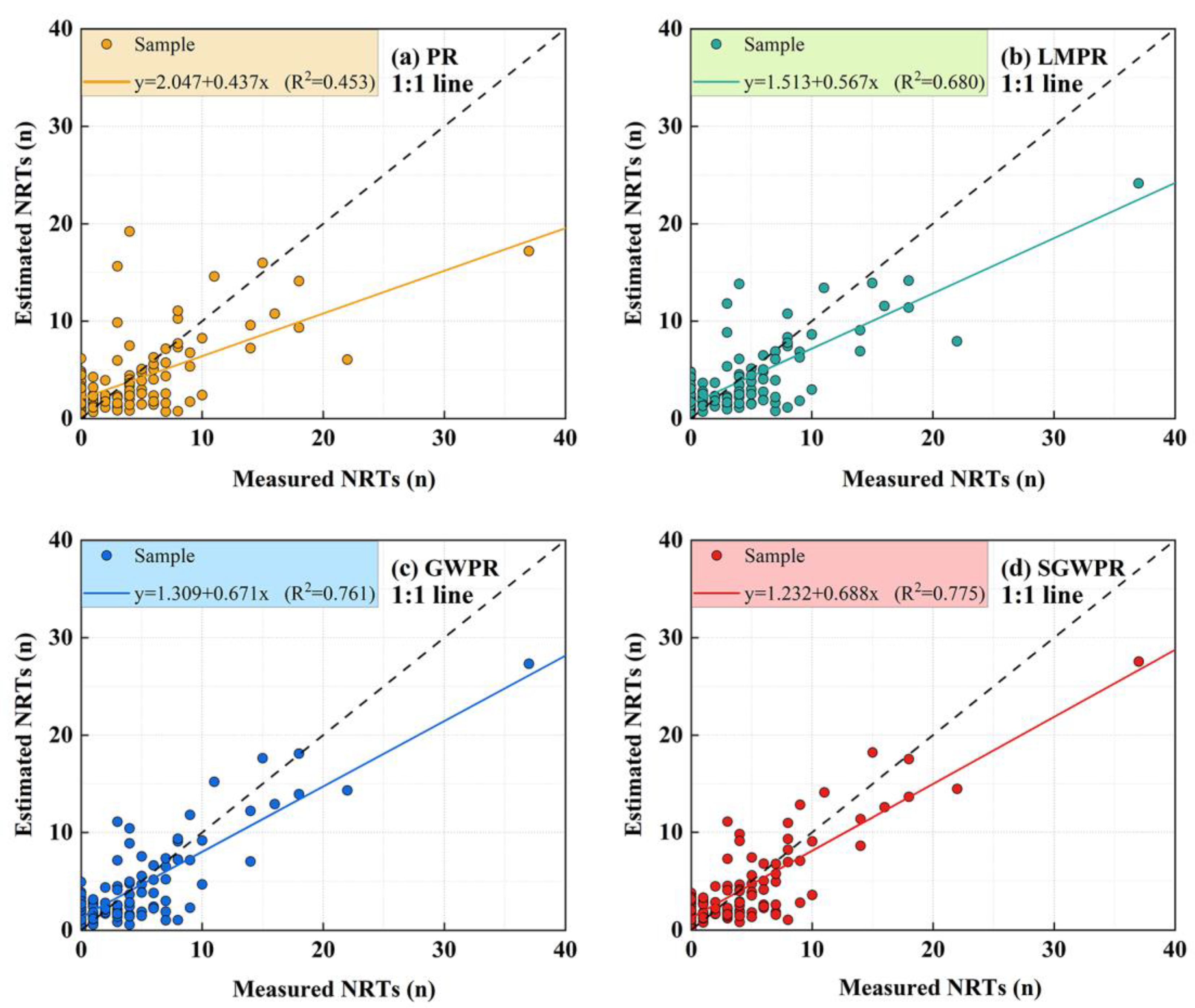
In this experiment, the fittings and predictive abilities of the four models were compared using the selected evaluation indicators. Table 5 shows that the models can be ranked in the order PR < LMPR < GWPR < SGWPR in both the training set and the validation set. In the training set, the local models had higher R2 values than the global models, and the RMSE and MAE values were much lower than those of the PR model. Compared with the GWPR model, the SGWPR model further improved the fitting and predictive abilities to a certain extent. Therefore, the occurrence of the optimal observed in the SGWPR model in this study indicates that not all variables need to be considered to be geographically variables. As shown in Figure 2, the 1:1 line fits of the local models were closer to the measured value and closer to the midline than those of the global models. The SGWPR model improved the accuracy of the GWPR model and had a good ability to solve the spatial autocorrelations of the model residuals, considering whether coefficients have geographical variability of all independent variables. Among the models employing principles of the LMPR, GWPR, and SGWPR, LMPR models were built by grouping the data in the global model, while the GWPR and SGWPR models were built by local searches. Both of these methods can improve the complexity and randomness in the data structure and the spatial effects of existing spatial data in the global PR model.

3.3. Residual Analysis

In this study, residual analyses were conducted on the four assessed models, as shown in Figure 3. The figure shows that the residual distribution ranges of the global (PR and LMPR) models were significantly larger than those of the local (GWPR and SGWPR) models, which indicated that the latter two models had better predictive ability than the former two. Moreover, it is noteworthy that the LMPR model, in which spatial effects are considered, performed much better than the PR model, with a significantly more concentrated residual distribution. Although the LMPR model can effectively improve the model capability, the results were not as good as those obtained using the local models. In addition, the PR model showed several strong influence points with large residual values, and local models improved the strong influence points.
Moran’s I value was computed to test the spatial autocorrelation in the residual error values (as shown in Table 6). When Moran’s I was set to zero, the residual distribution was completely spatially random. A standard normal test was used to determine whether the spatial distribution of the model residuals was random. If the normal test results in the value was −1.96 ≤ Z-statistic ≤ 1.96, then a p value > 0.05 indicated that the null hypothesis should be accepted. That is, the spatial distribution pattern of the model residuals was likely the result of randomness. Therefore, Table 6 shows that the PR model has difficulty eliminating spatial autocorrelation in the model residuals, while the residuals of the LMPR, GWPR, and SGWPR models show nonsignificant autocorrelations. According to the comparisons of the Z-statistic sizes performed in this study, the order of models in which spatial autocorrelation can be effectively eliminated is as follows: SGWPR, GWPR, and LMPR.
As shown in Figure 4, the spatial Moran I and Z statistic diagrams of the different models were drawn at intervals of 500 m. When the distance gradually increased, Moran’s I gradually and stably approached 0. Comparing the four models reveals that the PR model exhibited the largest variation in Moran’s I with distance, followed by the LMPR model. The GWPR and SGWPR models exhibited similar trends, but the SGWPR model value was closer to 0. In Figure 4b, which shows the Z statistic results, the shaded part covers the region from −1.96 to 1.96, and the area within this shadowed region includes significantly correlated residuals. Therefore, only the GWPR and SGWPR models have no significant autocorrelations at any distance.
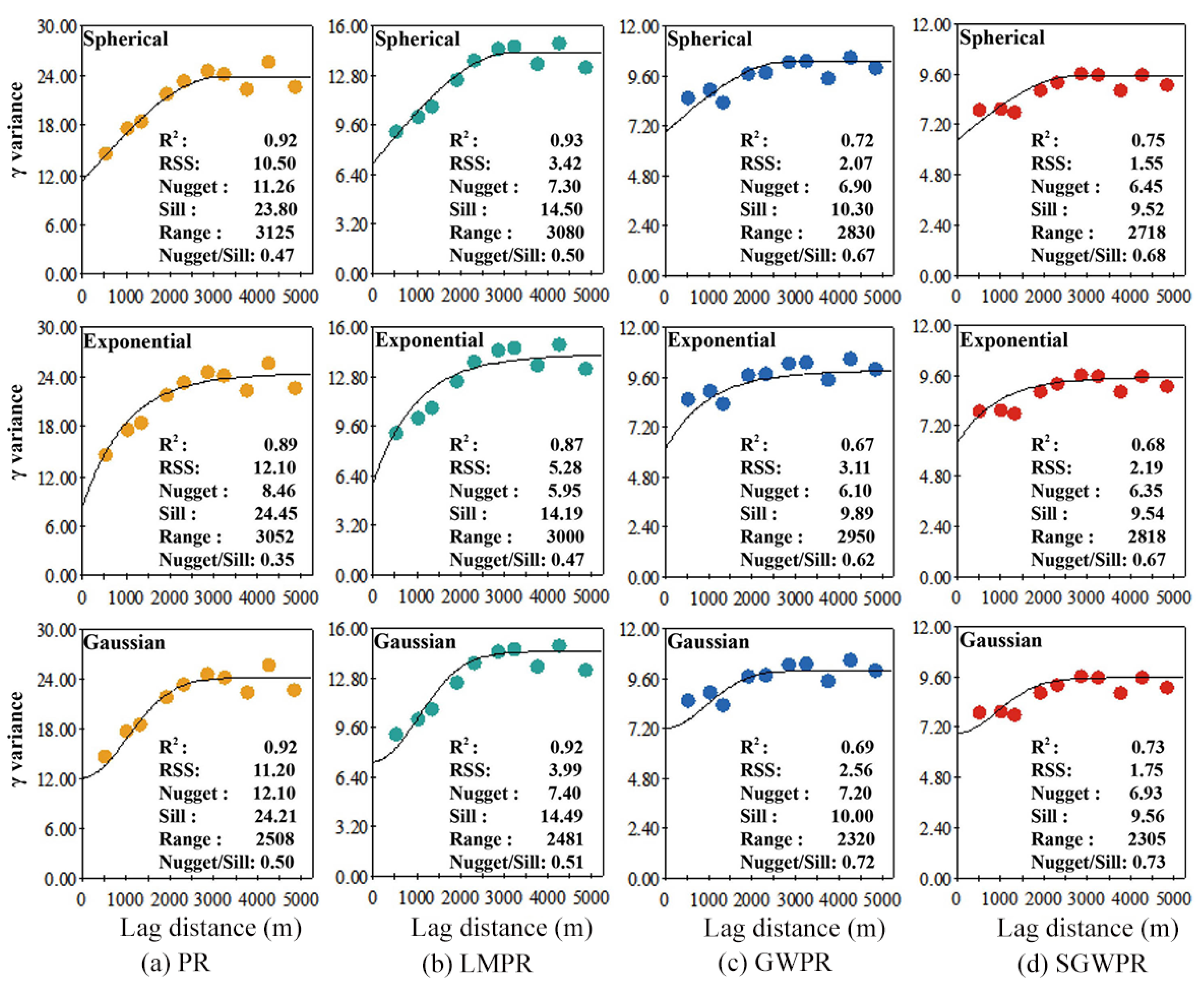
To further explain the spatial effect results, the spatial variability and structural characteristics of the residuals of different models were quantitatively reflected by using the range and nugget/sill values of spherical, exponential [58], and Gaussian functions in the geostatistical model variogram [59,60]. When it is necessary to distinguish the variance value of the variogram from variance in the general sense (independent of distance), “Gamma(γ) variance” is used. As shown in Figure 5, the optimally fitted model is the spherical model with the largest R2 value and the smallest RSS (residual sum of squares) value, followed by the Gaussian model, and finally the exponential model. From the optimal spherical function, the nugget/sill values of the global and local models are between 0.47 and 0.68, indicating that the residuals of the four models have moderate-intensity correlations. The smaller this value is, the stronger the correlation is. In general, the range is close to or greater than the sampling distance of 500 m set in this paper, indicating that the utilized sampling distance can effectively meet the research needs. When the range is large, it indicates that spatial correlation exists over a large range; the PR model had the largest range, while the SGWPR model had the smallest range. Moreover, the sill/nugget values of the SGWPR model were also the smallest among all models. That is, the SGWPR model results exhibit spatial correlation at a smaller distance than the other model results, and the correlation is small. This conclusion is confirmed by drawing Moran’s I correlation diagrams. In our study area, the spatial distances derived with a Moran index of 0 and the variation course calculated by the variation function are different due to the use of different calculation algorithms.

3.4. Visual Analysis

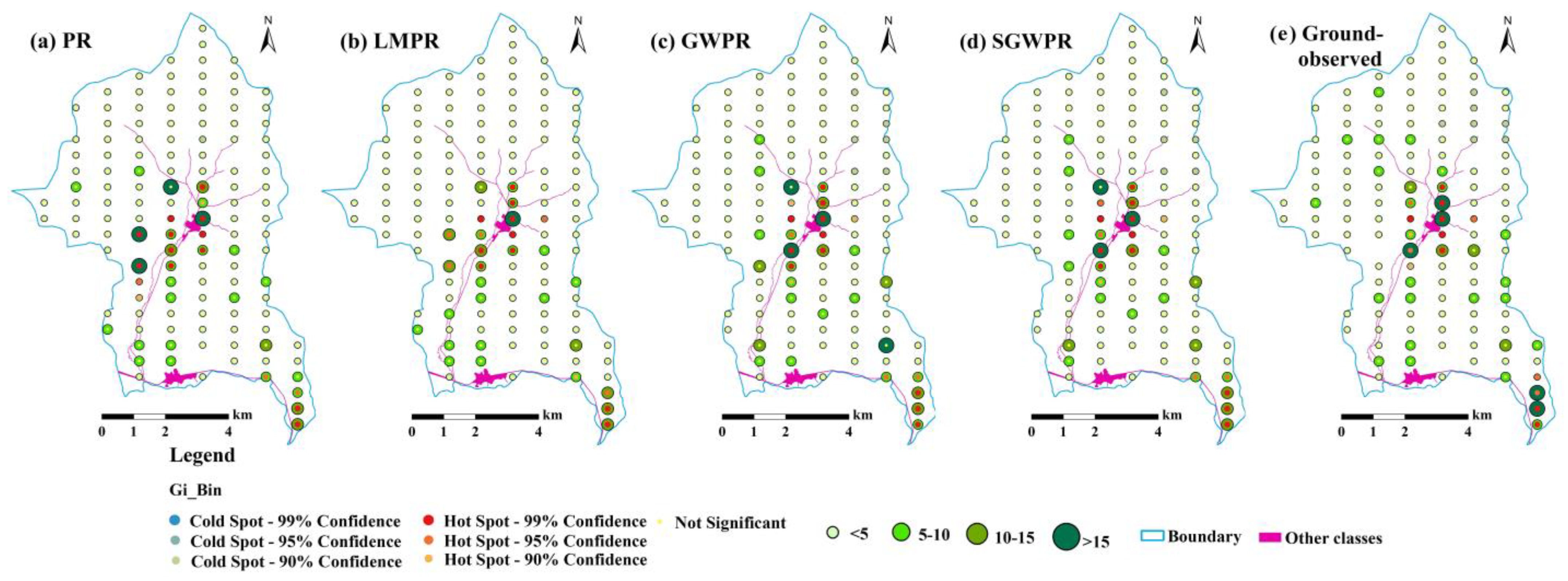
To observe the NRT results derived from the four different models more intuitively, we used a visual symbol system hierarchy and a hot spot analysis display of the studied nature reserve, thus allowing the spatial changes in the NRTs to be depicted in a more intuitive and detailed way. From the analysis of hot spots, we could see the distribution of high-value cluster points and low-value cluster points of the NRTs (Figure 6). As shown in Figure 6, higher NRT values were found in the middle and southeast of the study area, with values higher than 15 n, while smaller NRT values were found in the north and west, generally with values less than 5 n.
The SGWPR results were the most similar to the ground-observed results. Therefore, we also carried out IDW interpolation for the SGWPR model coefficients (Figure 7). The coefficients of the same variable show gradient changes in different spaces. When considering positive and negative values, the same variables showed different positive and negative correlations with the NRTs among different geographical regions, indicating that spatial nonstationarity existed in the stand environmental variables.

4. Discussion

4.1. Model Variables

Topography factors and the relationships between stand factors and recruitment are often considered when constructing NRT models. Remote sensing factors are seldom added when building such models. However, among the many studies on the spatial distributions of forest biomass and carbon storage, several studies have included VIs, textural features, and image-enhancement processes as variable factors [17,18,30]. These remote sensing factors can obtain simple, effective, and empirical surface vegetation status measurements, and are widely used in global and regional land cover, vegetation classification and environmental change, crop and pasture yield estimation, and monitoring research. In addition, these factors have been integrated into interactive biosphere models and productivity models as components of global climate models [17,18,30]. In this paper, topography, stand, and remote sensing factors were included when building the models for stepwise screening. Based on the fixed coefficients of the global models, it can be seen that the relationships between these factors and the NRTs are obvious. Among all variables, the estimated values of the NLTs and MNF2 coefficients were positive, indicating that these variables are positively correlated with the NRTs. The DEM, canopy, IPVI, and MeanB8 were negatively correlated with the NRTs. Overall, stand factors were more likely than other variables to be strongly correlated with the stand NRTs. In addition, the DEM variables were highly influential. Propastin [61] reported similar findings, which may have been the result of the utilized combination of topographic factors. Remote sensing factors were extracted from preprocessed Sentinel-2 images. The VIs of Sentinel-2 images are useful and common predictors, as has been confirmed by other researchers. These VIs can also be converted into leaf canopy biophysical parameters [62,63]. The effects of remote sensing factors on NRTs are not as significant as the effects of stand factors in global models [40]. However, in the local models it was evident that the potential results of these different methods may lead to changes in the directions and amplitudes of the resulting model coefficients, thus affecting the analysis interpretation results in different regions [1,64,65]. Some scholars found that climate change was also a key factor affecting the recruitment model. It has the potential to be an important tool for exploring the dynamic impact of climate change on forests in the future [5]. Larch NRTs may have benefited from colder winter temperatures, as saplings are less pathogenic [66]. Even climate warming is causing species migration, invasion and decline, which has seriously affected forest recruitment and structural changes [67]. The minimum growing period temperature and average annual temperature were positively correlated with the collection rate of conifers [68]. There have been few studies on the relationship between climate change and NRTs, which should be considered in the model in the future—including the impact of climate change, invasive species, insect pests, and fungi [69].

4.2. Model Comparisons

PR count data are often utilized in forestry and ecological environment research [43,44,70]. These data are collected from different geographic locations characterizing different geographical forest stand environments. However, research on which spatial characteristics should be considered when applying nonstationarity Poisson models in forestry and geographical ecology research is relatively scarce. In particular, it is difficult to make accurate predictions using the global PR model due to the complexity of stand NRT data. These data have a multilayer nested structure, autocorrelation among multiple observations, and a large number of 0 values [71,72], thus showing different degrees of discreteness and skewness relative to the mean [73]. At the same time, the spatial effects that exist in these data are complicated by their spatial autocorrelation and nonstationarity characteristics, which occur when the variables of interest are not independent of each other when located in adjacent positions [20]. Considering spatial nonstationarity, in this work, spatial data were analysed by modelling and were included in the regression framework to obtain optimal model parameter estimations, standard errors, and confidence interval deviations [74,75], and to improve the predictive abilities of the analysed models. Some studies have found that GLMMs (LMPR) [76,77] represent an improvement on nonmixed or nonspatial models because mixed models consider the spatial autocorrelations of the residuals of nonspatial models. Often, GLMMs (LMPR) are global models that can be used to effectively improve GLMs (PR), as has been reported in many articles. In one previous article, GLMMs (LMPR) did not show any improvement [47]. We believe that this occurred because the authors did not join the random effects (G matrix) and only considered the residual autocorrelation matrix using the distance R matrix, leading to anisotropy that cannot explain the residual of the GLMs (PR). In most cases, GLMMs (LMPR) are superior to GLMs (PR) [15,46] and even better than local models [14]. All the local models are better than the LMPR model in this study, possibly for the data. However, it is consistent with most studies [77,78]. It is worth noting that random sampling is used to select data. In the process of building GLMMs (LMPR), the locations of these random parameters differ, but this variation has little influence on the relevant results [79]. In terms of local models, the SGWPR model combines geographically varying (local coefficients) and fixed (global coefficients). This method is more flexible than GWPR; it can reduce the complexities of local relationships [52].
The SGWPR model improved the accuracy of the GWPR model and had a good ability to solve the spatial autocorrelations of the model residuals, considering whether coefficients have geographical variability of all independent variables. Among the models employing principles of the LMPR, GWPR, and SGWPR, LMPR models were built by grouping the data in the global model, while the GWPR and SGWPR models were built by local searches. Both of these methods can improve the complexity and randomness in the data structure and the spatial effects of existing spatial data in the global PR model [16,80].
To evaluate the abilities of the four analysed models to solve spatial data, Moran’s I and variogram function were introduced to the spatial effects of the model residuals [81]. Spatial effects may be caused by many ecological factors, such as distance-related biological processes, the absence of spatial structure-related environmental variables, and nonstationarity in the relationships between variables [82,83,84]. In this study, the PR models produced poor residual spatial autocorrelation and model residual distributions over short lag distances.

5. Conclusions

The Liangshui Nature Reserve in Northeast China contains original zonal vegetation consisting of mixed Pinus koraiensis broad-leaved forests. This region is the most typical and complete Pinus koraiensis broad-leaved forest ecosystem preserved in China. Thus, studying the responses and spatial distributions of the NRTs in this region and their response to driving factors such as topography, stand, and remote sensing factors by constructing theoretical models is a key factor for ensuring long-term forest maintenance, stand growth, and regeneration.
In this study, global (PR and LMPR) and local (GWPR and SGWPR) models were constructed to simulate NRT characteristics by using the Poisson correlation form. The R2 values of the GWPR and SGWPR models were 76% and 77% higher than that of the PR model, respectively. The SGWPR model produced good model-fitting, predictive abilities, and residual spatial effect results by considering whether coefficients have geographical variability of all independent variables in the GWPR model. This model provides more reliable technical support for accurately estimating the spatial distribution of NRTs, and is of great value for revealing the service functions of forest ecosystems and the sustainable and healthy development characteristics of forests.

Author Contributions

Conceptualization: Y.S.; methodology: Y.S.; software: Y.S. and H.G.; formal analysis: Y.S., F.W. and Z.Z.; investigation: H.Z. and T.L.; writing—original draft: Y.S. and X.Z.; supervision: W.J. All authors have read and agreed to the published version of the manuscript.

Funding

This study was funded by the National Natural Science Foundation of China, grant number 31870622, and the Special Fund Project for Basic Research in Central Universities, grant number 2572019CP08.

Data Availability Statement

The data presented in this study are available on request from the corresponding author.

Conflicts of Interest

The authors declare no conflict of interest.

References

  1. Zhen, Z.; Li, F.; Liu, Z.; Liu, C.; Zhao, Y.; Ma, Z.; Zhang, L. Geographically Local Modeling of Occurrence, Count, and Volume of Downwood in Northeast China. Appl. Geogr. 2013, 37, 114–126. [Google Scholar] [CrossRef]
  2. Chen, S.; Lu, N.; Fu, B.; Wang, S.; Deng, L.; Wang, L. Current and Future Carbon Stocks of Natural Forests in China. For. Ecol. Manag. 2022, 511, 120137. [Google Scholar] [CrossRef]
  3. Gauthier, M.; Guillemette, F.; Bédard, S. On the Relationship between Saplings and Ingrowth in Northern Hardwood Stands. For. Ecol. Manag. 2015, 358, 261–271. [Google Scholar] [CrossRef]
  4. Fortin, M.; DeBlois, J. Modeling Tree Recruitment with Zero-Inflated Models: The Example of Hardwood Stands in Southern Quebec, Canada. For. Sci. 2007, 53, 529–539. [Google Scholar]
  5. Xiang, W.; Lei, X.; Zhang, X. Modelling Tree Recruitment in Relation to Climate and Competition in Semi-Natural Larix-Picea-Abies Forests in Northeast China. For. Ecol. Manag. 2016, 382, 100–109. [Google Scholar] [CrossRef]
  6. Zhang, X.; Lei, Y.; Cai, D.; Liu, F. Predicting Tree Recruitment with Negative Binomial Mixture Models. For. Ecol. Manag. 2012, 270, 209–215. [Google Scholar] [CrossRef]
  7. Silla, F.; Camison, A.; Solana, A.; Hernandez, H.; Rios, G.; Cabrera, M.; Lopez, D.; Morera-Beita, A. Does the Persistence of Sweet Chestnut Depend on Cultural Inputs? Regeneration, Recruitment, and Mortality in Quercus- and Castanea-Dominated Forests. Ann. For. Sci. 2018, 75, 95. [Google Scholar] [CrossRef] [Green Version]
  8. Manso, R.; Ligot, G.; Fortin, M. A Recruitment Model for Beech-Oak Pure and Mixed Stands in Belgium. Forestry 2020, 93, 124–132. [Google Scholar] [CrossRef]
  9. Pardos, M.; Madrigal, G.; de Dios-García, J.; Gordo, J.; Calama, R. Sapling Recruitment in Mixed Stands in the Northern Plateau of Spain: A Patch Model Approach. Trees-Struct. Funct. 2021, 35, 2043–2058. [Google Scholar] [CrossRef]
  10. Russell, M.B.; Westfall, J.A.; Woodall, C.W. Modeling Browse Impacts on Sapling and Tree Recruitment across Forests in the Northern United States. Can. J. For. Res. 2017, 47, 1474–1481. [Google Scholar] [CrossRef]
  11. Russell, M.B. Influence of Prior Distributions and Random Effects on Count Regression Models: Implications for Estimating Standing Dead Tree Abundance. Environ. Ecol. Stat. 2015, 22, 145–160. [Google Scholar] [CrossRef]
  12. Zhang, X.-Q.; Lei, Y.-C.; Liu, X.-Z. Modeling Stand Mortality Using Poisson Mixture Models with Mixed-Effects. iForest 2015, 8, 333–338. [Google Scholar] [CrossRef] [Green Version]
  13. Zhou, X.; Fu, L.; Sharma, R.P.; He, P.; Lei, Y.; Guo, J. Generalized or General Mixed-Effect Modelling of Tree Morality of Larix Gmelinii Subsp. Principis-Rupprechtii in Northern China. J. For. Res. 2021, 32, 2447–2458. [Google Scholar] [CrossRef]
  14. Wei, Q.; Zhang, L.; Duan, W.; Zhen, Z. Global and Geographically and Temporally Weighted Regression Models for Modeling PM2.5 in Heilongjiang, China from 2015 to 2018. Int. J. Environ. Res. Public. Health 2019, 16, 5107. [Google Scholar] [CrossRef] [PubMed] [Green Version]
  15. Zhang, L.; Ma, Z.; Guo, L. An Evaluation of Spatial Autocorrelation and Heterogeneity in the Residuals of Six Regression Models. For. Sci. 2009, 55, 533–548. [Google Scholar] [CrossRef]
  16. Brunsdon, C.; Fotheringham, A.S.; Charlton, M.E. Geographically Weighted Regression: A Method for Exploring Spatial Nonstationarity. Geogr. Anal. 1996, 28, 281–298. [Google Scholar] [CrossRef]
  17. Foody, G.M. Geographical Weighting as a Further Refinement to Regression Modelling: An Example Focused on the NDVI-Rainfall Relationship. Remote Sens. Environ. 2003, 88, 283–293. [Google Scholar] [CrossRef]
  18. Foody, G.M.; Boyd, D.S.; Cutler, M.E.J. Predictive Relations of Tropical Forest Biomass from Landsat TM Data and Their Transferability between Regions. Remote Sens. Environ. 2003, 85, 463–474. [Google Scholar] [CrossRef]
  19. Propastin, P.A. Spatial Non-Stationarity and Scale-Dependency of Prediction Accuracy in the Remote Estimation of LAI over a Tropical Rainforest in Sulawesi, Indonesia. Remote Sens. Environ. 2009, 113, 2234–2242. [Google Scholar] [CrossRef]
  20. Tobler, W.R. A Computer Movie Simulating Urban Growth in the Detroit Region. Econ. Geogr. 1970, 46, 234–240. [Google Scholar] [CrossRef]
  21. Zhang, L.; Bi, H.; Cheng, P.; Davis, C.J. Modeling Spatial Variation in Tree Diameter–Height Relationships. For. Ecol. Manag. 2004, 189, 317–329. [Google Scholar] [CrossRef]
  22. Sun, Y.; Ao, Z.; Jia, W.; Chen, Y.; Xu, K. A Geographically Weighted Deep Neural Network Model for Research on the Spatial Distribution of the down Dead Wood Volume in Liangshui National Nature Reserve (China). iForest 2021, 14, 353–361. [Google Scholar] [CrossRef]
  23. Sun, Y.; Jia, W.; Zhu, W.; Zhang, X.; Saidahemaiti, S.; Hu, T.; Guo, H. Local Neural-Network-Weighted Models for Occurrence and Number of down Wood in Natural Forest Ecosystem. Sci. Rep. 2022, 12, 6375. [Google Scholar] [CrossRef] [PubMed]
  24. Zhang, X.; Sun, Y.; Jia, W.; Wang, F.; Guo, H.; Ao, Z. Research on the Temporal and Spatial Distributions of Standing Wood Carbon Storage Based on Remote Sensing Images and Local Models. Forests 2022, 13, 346. [Google Scholar] [CrossRef]
  25. Propastin, P. Modifying Geographically Weighted Regression for Estimating Aboveground Biomass in Tropical Rainforests by Multispectral Remote Sensing Data. Int. J. Appl. Earth Obs. Geoinf. 2012, 18, 82–90. [Google Scholar] [CrossRef]
  26. Battude, M.; Al Bitar, A.; Morin, D.; Cros, J.; Huc, M.; Marais Sicre, C.; Le Dantec, V.; Demarez, V. Estimating Maize Biomass and Yield over Large Areas Using High Spatial and Temporal Resolution Sentinel-2 like Remote Sensing Data. Remote Sens. Environ. 2016, 184, 668–681. [Google Scholar] [CrossRef]
  27. Astola, H.; Häme, T.; Sirro, L.; Molinier, M.; Kilpi, J. Comparison of Sentinel-2 and Landsat 8 Imagery for Forest Variable Prediction in Boreal Region. Remote Sens. Environ. 2019, 223, 257–273. [Google Scholar] [CrossRef]
  28. SNAP. Sentinels Application Platform, Software Version 4.0.0; European Space Agency: Paris, France, 2016. [Google Scholar]
  29. Chen, L.; Ren, C.; Zhang, B.; Wang, Z.; Xi, Y. Estimation of Forest Above-Ground Biomass by Geographically Weighted Regression and Machine Learning with Sentinel Imagery. Forests 2018, 9, 582. [Google Scholar] [CrossRef] [Green Version]
  30. Puliti, S.; Breidenbach, J.; Schumacher, J.; Hauglin, M.; Klingenberg, T.F.; Astrup, R. Above-Ground Biomass Change Estimation Using National Forest Inventory Data with Sentinel-2 and Landsat. Remote Sens. Environ. 2021, 265, 112644. [Google Scholar] [CrossRef]
  31. Huete, A.R. A Soil-Adjusted Vegetation Index (SAVI). Remote Sens. Environ. 1988, 25, 295–309. [Google Scholar] [CrossRef]
  32. Elvidge, C.D.; Chen, Z. Comparison of Broad-Band and Narrow-Band Red and near-Infrared Vegetation Indices. Remote Sens. Environ. 1995, 54, 38–48. [Google Scholar] [CrossRef]
  33. Myneni, R.B.; Tucker, C.J.; Asrar, G.; Keeling, C.D. Interannual Variations in Satellite-Sensed Vegetation Index Data from 1981 to 1991. J. Geophys. Res. Atmos. 1998, 103, 6145–6160. [Google Scholar] [CrossRef] [Green Version]
  34. Salas, E.A.L.; Henebry, G.M. A New Approach for the Analysis of Hyperspectral Data: Theory and Sensitivity Analysis of the Moment Distance Method. Remote Sens. 2014, 6, 20–41. [Google Scholar] [CrossRef] [Green Version]
  35. Sibanda, M.; Mutanga, O.; Rouget, M. Examining the Potential of Sentinel-2 MSI Spectral Resolution in Quantifying above Ground Biomass across Different Fertilizer Treatments. ISPRS J. Photogramm. Remote Sens. 2015, 110, 55–65. [Google Scholar] [CrossRef]
  36. Haralick, R.; Shanmugam, K.; Dinstein, I. Textural Features for Image Classification. IEEE Trans. Syst. Man Cybern. 1973, SMC3, 610–621. [Google Scholar] [CrossRef] [Green Version]
  37. Yang, C.; Lu, L.; Lin, H.; Guan, R.; Shi, X.; Liang, Y. A Fuzzy-Statistics-Based Principal Component Analysis (FS-PCA) Method for Multispectral Image Enhancement and Display. IEEE Trans. Geosci. Remote Sens. 2008, 46, 3937–3947. [Google Scholar] [CrossRef]
  38. Wulder, M.A.; Franklin, S.E.; Lavigne, M.B. High Spatial Resolution Optical Image Texture for Improved Estimation of Forest Stand Leaf Area Index. Can. J. Remote Sens. 1996, 22, 441–449. [Google Scholar] [CrossRef]
  39. Sarker, L.R.; Nichol, J.E. Improved Forest Biomass Estimates Using ALOS AVNIR-2 Texture Indices. Remote Sens. Environ. 2011, 115, 968–977. [Google Scholar] [CrossRef]
  40. Klopcic, M.; Poljanec, A.; Boncina, A. Modelling Natural Recruitment of European Beech (Fagus sylvatica L.). For. Ecol. Manag. 2012, 284, 142–151. [Google Scholar] [CrossRef]
  41. Axer, M.; Martens, S.; Schlicht, R.; Wagner, S. Modelling Natural Regeneration of European Beech in Saxony, Germany: Identifying Factors Influencing the Occurrence and Density of Regeneration. Eur. J. For. Res. 2021, 140, 947–968. [Google Scholar] [CrossRef]
  42. Guisan, A.; Edwards, T.C.; Hastie, T. Generalized Linear and Generalized Additive Models in Studies of Species Distributions: Setting the Scene. Ecol. Model. 2002, 157, 89–100. [Google Scholar] [CrossRef] [Green Version]
  43. Podur, J.J.; Martell, D.L.; Stanford, D. A Compound Poisson Model for the Annual Area Burned by Forest Fires in the Province of Ontario. Environmetrics 2010, 21, 457–469. [Google Scholar] [CrossRef]
  44. Ma, Z.; Zuckerberg, B.; Porter, W.F.; Zhang, L. Spatial Poisson Models for Examining the Influence of Climate and Land Cover Pattern on Bird Species Richness. For. Sci. 2012, 58, 61–74. [Google Scholar] [CrossRef]
  45. Schabenberger, O. Introducing the GLIMMIX Procedure for Generalized Linear Mixed Models. Statistics and Data Analysis. Statistics and Data Analysis. SUGI 2008, 30, 196–230. [Google Scholar]
  46. Zhang, L.; Gove, J.H.; Heath, L.S. Spatial Residual Analysis of Six Modeling Techniques. Ecol. Model. 2005, 186, 154–177. [Google Scholar] [CrossRef]
  47. Wu, W.; Zhang, L. Comparison of Spatial and Non-Spatial Logistic Regression Models for Modeling the Occurrence of Cloud Cover in North-Eastern Puerto Rico. Appl. Geogr. 2013, 37, 52–62. [Google Scholar] [CrossRef]
  48. Shi, H.; Zhang, L.; Liu, J. A New Spatial-Attribute Weighting Function for Geographically Weighted Regression. Can. J. For. Res. 2006, 36, 996–1005. [Google Scholar] [CrossRef] [Green Version]
  49. Griffith, D.A. Spatial-Filtering-Based Contributions To A Critique Of Geographically Weighted Regression (Gwr). Environ. Plan. 2008, 40, 2751–2769. [Google Scholar] [CrossRef]
  50. Usman, U.; Yelwa, S.A.; Gulumbe, S.U.; Danbaba, A. Modelling Relationship between NDVI and Climatic Variables Using Geographically Weighted Regression. J. Math. Sci. Appl. 2013, 1, 24–28. [Google Scholar] [CrossRef]
  51. Shin, J.; Temesgen, H.; Strunk, J.L.; Hilker, T. Comparing Modeling Methods for Predicting Forest Attributes Using LiDAR Metrics and Ground Measurements. Can. J. Remote Sens. 2016, 42, 739–765. [Google Scholar] [CrossRef]
  52. Nakaya, T. Geographically Weighted Generalised Linear Modelling. In Geocomputation: A Practical Primer; SAGE Publications Ltd.: New York, NY, USA, 2015; pp. 201–220. ISBN 978-1-4462-7292-3. [Google Scholar]
  53. Anselin, L. Spatial Effects in Econometric Practice in Environmental and Resource Economics. Am. J. Agric. Econ. 2001, 83, 705–710. [Google Scholar] [CrossRef]
  54. de Jong, P.; Sprenger, C.; van Veen, F. On Extreme Values of Moran’s I and Geary’s c. Geogr. Anal. 1984, 16, 17–24. [Google Scholar] [CrossRef]
  55. Sawada, M. Rookcase: An Excel 97/2000 Visual Basic (VB) Add-in for Exploring Global and Local Spatial Autocorrelation. Bull. Ecol. Soc. Am. 1999, 80, 231–234. [Google Scholar] [CrossRef]
  56. Hu, T.; Sun, Y.; Jia, W.; Li, D.; Zou, M.; Zhang, M. Study on the Estimation of Forest Volume Based on Multi-Source Data. Sensors 2021, 21, 7796. [Google Scholar] [CrossRef]
  57. Barnes, R.J. The Variogram Sill and the Sample Variance. Math. Geol. 1991, 23, 673–678. [Google Scholar] [CrossRef]
  58. Solana-Gutiérrez, J.; Merino-de-Miguel, S. A Variogram Model Comparison for Predicting Forest Changes. Procedia Environ. Sci. 2011, 7, 383–388. [Google Scholar] [CrossRef] [Green Version]
  59. Bachmaier, M.; Backes, M. Variogram or Semivariogram? Understanding the Variances in a Variogram. Precis. Agric. 2008, 9, 173–175. [Google Scholar] [CrossRef]
  60. Strîmbu, V.F.; Ene, L.T.; Næsset, E. Spatially Consistent Imputations of Forest Data under a Semivariogram Model. Can. J. For. Res. 2016, 46, 1145–1156. [Google Scholar] [CrossRef] [Green Version]
  61. Propastin, P. Multiscale Analysis of the Relationship between Topography and Aboveground Biomass in the Tropical Rainforests of Sulawesi, Indonesia. Int. J. Geogr. Inf. Sci. 2011, 25, 455–472. [Google Scholar] [CrossRef]
  62. Sprintsin, M.; Karnieli, A.; Berliner, P.; Rotenberg, E.; Yakir, D.; Cohen, S. The Effect of Spatial Resolution on the Accuracy of Leaf Area Index Estimation for a Forest Planted in the Desert Transition Zone. Remote Sens. Environ. 2007, 109, 416–428. [Google Scholar] [CrossRef]
  63. Taureau, F.; Robin, M.; Proisy, C.; Fromard, F.; Imbert, D.; Debaine, F. Mapping the Mangrove Forest Canopy Using Spectral Unmixing of Very High Spatial Resolution Satellite Images. Remote Sens. 2019, 11, 367. [Google Scholar] [CrossRef] [Green Version]
  64. Fotheringham, A.S.; Charlton, M.; Brunsdon, C. Two Techniques for Exploring Non-Stationarity in Geographical Data. Geogr. Syst. 1997, 4, 59–82. [Google Scholar]
  65. Demšar, U.; Fotheringham, S.A.; Charlton, M. Combining Geovisual Analytics with Spatial Statistics: The Example of Geographically Weighted Regression. Cartogr. J. 2008, 45, 182–192. [Google Scholar] [CrossRef] [Green Version]
  66. Packer, A.; Clay, K. Soil Pathogens and Prunus Serotina Seedling and Sapling Growth Near Conspecific Trees. Ecology 2003, 84, 108–119. [Google Scholar] [CrossRef]
  67. Peñuelas, J.; Ogaya, R.; Boada, M.; Jump, A.S. Migration, Invasion and Decline: Changes in Recruitment and Forest Structure in a Warming-Linked Shift of European Beech Forest in Catalonia (NE Spain). Ecography 2007, 30, 829–837. [Google Scholar] [CrossRef]
  68. Vitasse, Y.; Hoch, G.; Randin, C.F.; Lenz, A.; Kollas, C.; Körner, C. Tree Recruitment of European Tree Species at Their Current Upper Elevational Limits in the Swiss Alps. J. Biogeogr. 2012, 39, 1439–1449. [Google Scholar] [CrossRef]
  69. Dyderski, M.K.; Paź, S.; Frelich, L.E.; Jagodziński, A.M. How Much Does Climate Change Threaten European Forest Tree Species Distributions? Glob. Chang. Biol. 2018, 24, 1150–1163. [Google Scholar] [CrossRef]
  70. Jones, M.T.; Niemi, G.J.; Hanowski, J.M.; Regal, R.R. Poisson Regression: A Better Approach to Modeling Abundance Data. In Predicting Species Occurrences: Issues of Accuracy and Scale, 1st ed.; Scott, J.M., Heglund, P.J., Morrison, M.L., Haufler, J.B., Raphael, M.G., Wall, W.A., Samson, F.B., Eds.; Island Press: Washington, DC, USA, 2002; pp. 411–418. [Google Scholar]
  71. Rathbun, S.L.; Fei, S. A Spatial Zero-Inflated Poisson Regression Model for Oak Regeneration. Environ. Ecol. Stat. 2006, 13, 409. [Google Scholar] [CrossRef]
  72. Zuur, A.F.; Ieno, E.N.; Elphick, C.S. A Protocol for Data Exploration to Avoid Common Statistical Problems. Methods Ecol. Evol. 2010, 1, 3–14. [Google Scholar] [CrossRef]
  73. Li, R.; Weiskittel, A.R.; Kershaw, J.A. Modeling Annualized Occurrence, Frequency, and Composition of Ingrowth Using Mixed-Effects Zero-Inflated Models and Permanent Plots in the Acadian Forest Region of North America. Can. J. For. Res. 2011, 41, 2077–2089. [Google Scholar] [CrossRef]
  74. Cunningham, R.B.; Lindenmayer, D.B. Modeling Count Data of Rare Species: Some Statistical Issues. Ecology 2005, 86, 1135–1142. [Google Scholar] [CrossRef]
  75. Lindén, A.; Mäntyniemi, S. Using the Negative Binomial Distribution to Model Overdispersion in Ecological Count Data. Ecology 2011, 92, 1414–1421. [Google Scholar] [CrossRef]
  76. Kéry, M.; Royle, J.A.; Schmid, H. Modeling Avian Abundance from Replicated Counts Using Binomial Mixture Models. Ecol. Appl. 2005, 15, 1450–1461. [Google Scholar] [CrossRef]
  77. Zhang, L.; Ma, Z.; Guo, L. Spatially Assessing Model Errors of Four Regression Techniques for Three Types of Forest Stands. Forestry 2008, 81, 209–225. [Google Scholar] [CrossRef] [Green Version]
  78. Zhang, L.; Gove, J.H. Spatial Assessment of Model Errors from Four Regression Techniques. For. Sci. 2005, 51, 334–346. [Google Scholar]
  79. Guo, H.; Jia, W.; Li, D.; Sun, Y. Modeling Knot Geometry from Scanned Images of Korean Pine Plantations. Can. J. For. Res. 2022, 52, 845–859. [Google Scholar] [CrossRef]
  80. Harris, P.; Brunsdon, C. Exploring Spatial Variation and Spatial Relationships in a Freshwater Acidification Critical Load Data Set for Great Britain Using Geographically Weighted Summary Statistics. Comput. Geosci. 2010, 36, 54–70. [Google Scholar] [CrossRef]
  81. Johnson, D.J.; Magee, L.; Pandit, K.; Bourdon, J.; Broadbent, E.N.; Glenn, K.; Kaddoura, Y.; Machado, S.; Nieves, J.; Wilkinson, B.E.; et al. Canopy Tree Density and Species Influence Tree Regeneration Patterns and Woody Species Diversity in a Longleaf Pine Forest. For. Ecol. Manag. 2021, 490, 119082. [Google Scholar] [CrossRef]
  82. Carl, G.; Kühn, I. Analyzing Spatial Autocorrelation in Species Distributions Using Gaussian and Logit Models. Ecol. Model. 2007, 207, 159–170. [Google Scholar] [CrossRef]
  83. Dormann, C.F.; McPherson, J.M.; Araújo, M.B.; Bivand, R.; Bolliger, J.; Carl, G.; Davies, R.G.; Hirzel, A.; Jetz, W.; Kissling, W.D.; et al. Methods to Account for Spatial Autocorrelation in the Analysis of Species Distributional Data: A Review. Ecography 2007, 30, 609–628. [Google Scholar] [CrossRef] [Green Version]
  84. Griffith, D.; Chun, Y. Spatial Autocorrelation and Spatial Filtering. In Handbook of Regional Science; Fischer, M.M., Nijkamp, P., Eds.; Springer: Berlin/Heidelberg, Germany, 2014; pp. 1477–1507. ISBN 978-3-642-23430-9. [Google Scholar]
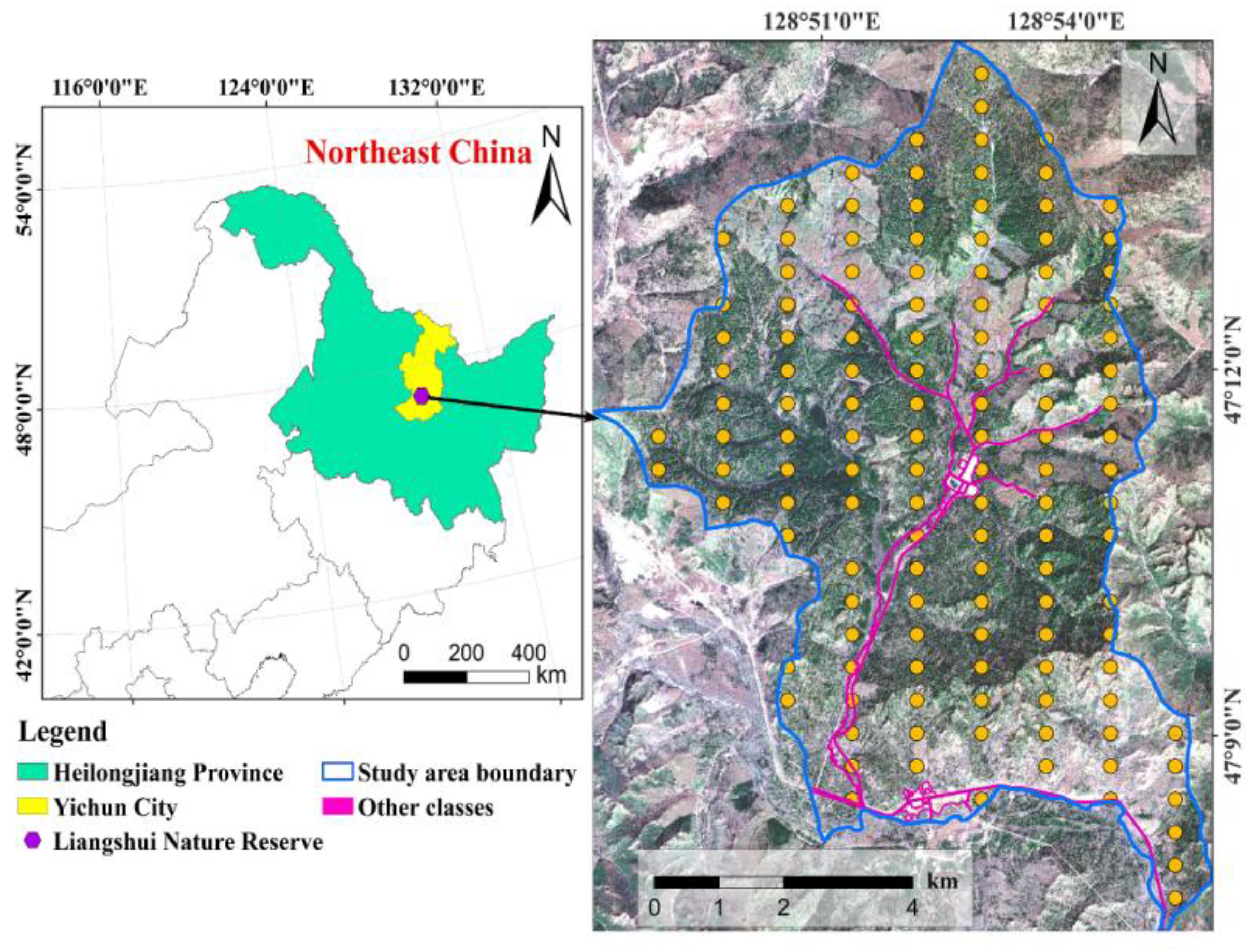
Figure 1. Overview of the Northeast China Liangshui Nature Reserve study area and the distribution of sample plots.
Forests 14 00739 g001
Figure 2. Scatter diagrams of the estimated NRTs (n) and the measured NRTs (n) by the four models. (a) PR represents the Poisson regression, (b) LMPR represents the Liner mixed PR, (c) GWPR represents the Geographically weighted PR, and (d) SGWPR represents the semiparametric GWPR. Note: NRTs represents the number of recruitment trees. The dotted line in the figure is the median line, the point is the measured and estimated NRTs, and the color line is the fitting line. The closer the color line is to the median line, the better the model is.
Forests 14 00739 g002
Figure 3. Residual boxplots of the four assessed models: global ((a) PR represents the Poisson regression and (b) LMPR represents the Liner mixed PR) models and local ((c) GWPR represents the Geographically weighted PR and (d) SGWPR represents the semiparametric GWPR) models.
Forests 14 00739 g003
Figure 4. (a) Moran’s I and (b) Z statistic of the residual analysed at different lag distances. Note: PR represents the Poisson regression, LMPR represents the Liner mixed PR, GWPR represents the Geographically weighted PR, SGWPR represents the semiparametric GWPR.
Forests 14 00739 g004
Figure 5. The nugget, sill, and nugget/sill parameters of the analysed global and local models, including the models built using spherical, exponential, and Gaussian functions. (a) PR represents the Poisson regression, (b) LMPR represents the Liner mixed PR, (c) GWPR represents the Geographically weighted PR, and (d) SGWPR represents the semiparametric GWPR. Note: The black line in the figure is a Spherical, Exponential and Gaussian fitting line.
Forests 14 00739 g005
Figure 6. Visual and hotspot analysis of the NRT prediction results obtained from the four models and the ground-observed values. (a) PR represents the Poisson regression, (b) LMPR represents the Liner mixed PR, (c) GWPR represents the Geographically weighted PR, (d) SGWPR represents the semiparametric GWPR, and (e) Ground-observed data. Note: NRTs represents the number of recruitment trees.
Forests 14 00739 g006
Figure 7. Coefficient visualization analysis of the SGWPR local variables: (a) intercept, (b) DEM, (c) NLTs, (d) canopy, and (e) MNF2. Note: IPVI represents the Infrared Percentage vegetation index, MeanB8 represents the B8 mean textural feature analysis, MNF2 represents the second minimum noise fraction (MNF) of sentinel 2, PR represents the Poisson regression, LMPR represents the Liner mixed PR, GWPR represents the Geographically weighted PR, SGWPR represents the semiparametric GWPR.
Forests 14 00739 g007
Table 1. Remote sensing image extraction factors.
Remote Sensing FactorsDescriptionAbbreviation
VIRatio VIB8/B4RVI
Atmospheric Ratio VI[B8 − (2 × B4 − B2)]/[B8 + (2 × B4 − B2)]ARVI
Difference VIB8 − B4DVI
Weighted Difference VIB8 − 0.8 × B4WDVI
Perpendicular VIsin 45° × B8 − cos 45° × B4PVI
Infrared Percentage VIB8/(B8 + B4)IPVI
Normalized Difference VI(B8 − B4)/(B8 − B4)NDVI
Soil-Adjusted VI1.5 × (B8 − B4)/8 × (B8 + B4 + 0.5)SAVI
Modified Soil-Adjusted VI(2 − NDVI × WDVI) × (B8 − B4)/8 × (B8 + B4 + 1 − NDVI × WDVI)MSAVI
Modified Soil-Adjusted VI20.5 × (2 × (B8 + 1)) − sqrt[(2 × B8 + 1)2 − 8 × (B8 − B4)]MSAVI2
TexturalMeanB4 and B8MeanB4 and MeanB8
VarianceB4 and B8VarB4 and VarB8
HomogeneityB4 and B8HomoB4 and HomoB8
ContrastB4 and B8ConB4 and ConB8
EntropyB4 and B8EntrB4 and EntrB8
Second momentB4 and B8SMB4 and SMB8
CorrelationB4 and B8CorrB4 and CorrB8
Image
enhancement
Minimum noise fractionThe first three minimum noise fractionMNF1, MNF2 and MNF3
Principal component analysisThe first three principal components analysisPCA1, PCA2 andPCA3
Note: VI represents the vegetation index. B2, B4, and B8 represent blue, infrared, and near-infrared bands, respectively.
Table 2. Basic statistical indicators of the model variables.
VariableMeanMedianStdMinMaxCVVIF
DEM (m)402.12390.0076.72270.00638.0019.081.04
Number of living trees (NLTs, nha-1)702.63633.33406.5683.332716.6757.861.79
Canopy0.530.500.140.300.9025.491.81
IPVI0.780.780.060.690.897.0311.02
MeanB824.5424.562.0419.7830.788.331.02
MNF20.170.165.7515.0911.933422.251.02
Number of recruitment trees (NRTs, n)3.732.005.290.0037.00141.79-
Note: IPVI represents the Infrared Percentage vegetation index, MeanB8 represents the B8 mean textural feature analysis, MNF2 represents the second minimum noise fraction (MNF) of sentinel 2.
Table 3. Global and local model coefficient estimates.
ModelsStatisticsInterceptDEMNLTsCanopyIPVIMeanB8MNF2
PREstimate0.952−0.3530.600−0.615−0.322−0.4010.331
p value<0.0001<0.0001<0.0001<0.0001<0.0001<0.0001<0.0001
LMPREstimate0.930−0.3680.601−0.620−0.283−0.3820.255
p value<0.00010.003<0.00010.0020.0050.0160.047
GWPRMean0.947−0.4680.643−0.686−0.248−0.3720.271
Min0.527−1.189−0.159−1.627−0.458−0.619−0.095
Q10.788−0.6590.290−1.165−0.360−0.4460.099
Median0.984−0.4330.673−0.589−0.264−0.3670.336
Q31.090−0.2270.999−0.311−0.151−0.2860.406
Max1.374−0.1061.4760.3510.094−0.1490.612
SGWPRMean0.944−0.4550.645−0.693−0.306−0.3770.239
Min0.520−1.184−0.153−1.579−0.094
Q10.746−0.6320.302−1.1700.113
Median0.955−0.4210.649−0.6160.205
Q31.123−0.2231.043−0.3080.393
Max1.370−0.1131.3710.3470.599
Note: IPVI represents the Infrared Percentage vegetation index, MeanB8 represents the B8 mean textural feature analysis, MNF2 represents the second minimum noise fraction (MNF) of sentinel 2. PR represents the Poisson regression, LMPR represents the Liner mixed PR, GWPR represents the Geographically weighted PR, SGWPR represents the semiparametric GWPR.
Table 4. Statistics for the geographical variability tests of the GWPR model for local terms.
Δ D k ∆DOF Δ A I C c k
Intercept14.4451.772−8.488
DEM19.2981.416−14.515
NLTs38.7871.282−34.449
Canopy30.6841.706−24.942
IPVI8.7982.514−0.427
MeanB81.9351.6003.457
MNF210.0551.814−3.960
Note: IPVI represents the Infrared Percentage vegetation index, MeanB8 represents the B8 mean textural feature analysis, MNF2 represents the second minimum noise fraction (MNF) of sentinel 2.
Table 5. Statistics of the evaluation indicators in the training and validation sets of the assessed global and local models.
ModelsTraining SetValidation Set
R2RMSEMAEAICcBICR2RMSEMAEP%
PR0.4534.5872.699366.967383.6450.4403.2792.55867.488
LMPR0.6953.4292.287--0.4503.2482.53468.587
GWPR0.7972.7961.919266.176308.9890.4573.2272.44671.721
SGWPR0.8032.7821.918262.402298.9070.5113.0622.41372.335
Note: PR represents the Poisson regression, LMPR represents the Liner mixed PR, GWPR represents the Geographically weighted PR, SGWPR represents the semiparametric GWPR.
Table 6. Global Moran’s I, Z-statistic, and p value statistical analysis results of the four models.
ModelsPRLMPRGWPRSGWPR
Moran’s I0.1960.0920.0210.011
Z-statistic2.1781.0690.3140.201
p value0.0290.2850.7540.841
Note: PR represents the Poisson regression, LMPR represents the Liner mixed PR, GWPR represents the Geographically weighted PR, SGWPR represents the semiparametric GWPR.
Disclaimer/Publisher’s Note: The statements, opinions and data contained in all publications are solely those of the individual author(s) and contributor(s) and not of MDPI and/or the editor(s). MDPI and/or the editor(s) disclaim responsibility for any injury to people or property resulting from any ideas, methods, instructions or products referred to in the content.