Article

Biomass Models and Ecosystem Carbon Density: A Case Study of Two Coniferous Forest in Northern Hunan, China

1
College of Forestry, Central South University of Forestry & Technology, Changsha 410004, China
2
Hunan Huarong Donghu National Wetland Park, Yueyang 414201, China
*
Author to whom correspondence should be addressed.
Forests 2023, 14(4), 814; https://doi.org/10.3390/f14040814
Submission received: 22 February 2023 / Revised: 6 April 2023 / Accepted: 12 April 2023 / Published: 15 April 2023
(This article belongs to the Section Forest Ecology and Management)

Abstract

:
The carbon sink capacity of forest ecosystem and its function of mitigating climate change have been confirmed. As two common coniferous species, Cunninghamia lanceolata (Lamb.) Hook. (C. lanceolata) and Pinus elliottii Engelmann (P. elliottii) are widely planted in southern China, and their carbon sink capacity has always been concerning. According to their diameter class, we randomly harvested 42 C. lanceolata trees and 38 P. elliottii trees from our entire study area, measured their carbon concentration, and constructed biomass models with DBH and tree height as variables. The biomass of the tree layer was estimated by measuring the DBH of all trees in the plots, and the biomass and carbon concentration of shrubs, herbs, dead wood and litter in the plot were measured by harvesting them. The results showed that the total biomass in C. lanceolata and P. elliottii plantations were 117.1 and 151.8 t·ha−1; the biomass in the tree layer was 94.7 and 122.9 t·ha−1; and in the other parts was 22.4 and 28.9 t·ha−1, respectively. In addition, the total carbon densities in the C. lanceolata and P. elliottii plantation ecosystems were 166.3 and 198.6 t·ha−1; the carbon densities in the soil were 108.1 and 124.6 t·ha−1; and in the other parts, they were 58.2 and 74.0 t·ha−1, respectively. These results indicate that there are significant differences in total biomass or total carbon storage between the two coniferous forest ecosystems, and net productivity and carbon sink capacity are higher in the P. elliottii plantation ecosystem. This study lays the foundation for the biomass estimation and carbon trading of these two coniferous forests in northern Hunan.

1. Introduction

Global climate change has threatened global organisms and the ecological environment on which they depend [1], and also affected the survival and sustainable development of mankind [2,3]. The greenhouse effect and the warming climate have made forest carbon sinks increasingly valued by humans [4,5]. Forests are the main parts of the terrestrial ecosystem, and their annual carbon sink was about 2.4 ± 0.4 Pg from 1990 to 2007, which was about 2/3 of the total terrestrial ecosystem [4]. Forests play an irreplaceable role in regulating the global carbon balance, mitigating the increase in greenhouse gas concentrations such as CO2 in the atmosphere, and addressing climate change [6,7]. However, harvests, forest fire, drought and other factors will affect the carbon balance in a certain time and space [8,9,10]. Therefore, the study of the forest ecosystem carbon balance is of great significance for scientifically predicting the role of forests in the global carbon balance and climate change.
With global carbon emission reduction actions, the research of forest carbon storage has attracted the attention of domestic and foreign scholars. In the mid-to-late 1960s, the International Biological Program (IBP) from the International Council of Scientific Unions (ICSU) carried out research on carbon sinks in terrestrial forest ecosystems [11]. In the late 1990s, the signing of the ‘Kyoto Protocol’ made the economy and trade related to forest carbon sinks valued by the international community [12]. Such research also boomed after 2007 [13]. The biomass method [14], model method [15], stable isotope method [16,17] and remote sensing inversion method [18,19] are the main methods to estimate forest carbon storage at present. In 2018, China’s annual average carbon sequestration was 2.3 × 10⁸ t·yr−1, which was 2.9 times that of 1978 [20]. With the expansion of coniferous or broad-leaved plantations, the amount of forest carbon sequestration continues to increase in China [15,21].
From 1990 to 2015, the global cumulative artificial afforestation area reached 1.2 × 10⁸ ha, accounting for the proportion of the world’s total forest area increasing from 4.1% to 7.3% [22]. According to the data of the eighth forest resources inventory in China, the planted area reached 0.69 × 10⁸ ha, accounting for 33% of that in the world [23]. In addition, the main tree species for afforestation include Chinese fir (C. lanceolata), Populus spp., Pinus massoniana Lamb., slash pine (P. elliottii), Eucalyptus spp., Quercus spp. and Betula spp. [24]. Among them, C. lanceolata and P. elliottii are two important coniferous timber forest species, which are widely planted in the hilly areas of southern China, with an excellent carbon sequestration capacity [25,26]. The biomass, net primary productivity and carbon storage of the two coniferous forests have been widely reported but reports mainly concentrated on the tree and soil of the forest [27,28,29]. Few studies have involved the carbon storage of the understory vegetation and the litter layer, especially dead wood.
In this study, forest ecosystem carbon storage was divided into five parts: the tree layer, understory vegetation (shrub layer and herb layer), dead wood, litter layer and soil. The biomass models of C. lanceolata and P. elliottii were constructed from standard trees, Next, the biomass in a standard plot was calculated from the models, and the carbon density of the tree layer was further calculated. The carbon density of understory vegetation, dead wood and the litter layer was estimated using the total harvest method. Forest soil carbon density was estimated using soil carbon concentration, bulk density and depth. The purpose of this paper is to compare the carbon density of the two principal coniferous forests (including vegetation, litter layer and soil), estimate the forest ecosystem carbon storage in Northern Hunan, and lay the foundation for forest carbon trading.

2. Materials and Methods

2.1. Study Area

The research site is located in the Shengfeng and Tashi state-owned forest farms in Huarong County, Hunan Province, China (112°40′–112°52′ E, 29°33′–29°40′ N) (Figure 1). This region has a typical subtropical monsoon climate, with a mean annual temperature of 17.2 °C, mean annual precipitation of 1189 mm, 1517 h hours of sunshine, and a mean annual frost-free period of 262 d. Forests are mainly distributed in low mountain and hilly areas, with an altitude of 95–382 m above sea level and a slope of <30°. The zonal soil is mainly red soil, accompanied by a small amount of rock debris, with a thickness of 0.7–1.0 m. In the state-owned forest farms, C. lanceolata, P. elliottii, Cinnamomum camphora (L.) Presl, Liquidambar formosana Hance, and some economic tree species such as Citrus reticulata Blanco, Castanea mollissima Bl. and Camellia oleifera Abel, are planted, among which the planting areas of C. lanceolata and P. elliottii account for 47% and 35%, respectively.

2.2. Sample Plot Setting

In August 2022, four C. lanceolata plots and four P. elliottii plots were established in the state-owned forest farms (Figure 1), with a size of 20 m × 30 m and a tree age of 19. (i) We measured the DBH (diameter at breast height at a height of 1.3 m) of all trees on the 8 plots. (ii) We established three 2 m × 2 m quadrats along the diagonal in each plot, with a total of 24, and harvested all shrubs (C. lanceolata or P. elliottii with a DBH of < 6 cm are also regarded as shrubs) and all herbs in each quadrat. (iii) Next, we set three 1 m × 1 m small quadrats along another diagonal in each plot, with a total of 24, and harvested all the litter in each small quadrat, according to ‘undecomposed’, ‘semi-decomposed’ and ‘decomposed’. Table 1 indicates the structural characteristics of the two coniferous forest plots.

2.3. Biomass Model Construction

In order to reduce damage to forests, we harvested 42 C. lanceolata trees and 38 P. elliottii trees in state-owned forest farms (excluding plots), there was a large distance between the harvested trees, which were about half the number of trees in a plot. (i) We measured the DBH and the height of these trees. (ii) We divided all trees into stems, branches, leaves, fruits and roots using Monsic′s stratified clip method [30,31]. Then, the fresh weight of each component of these trees was measured. (iii) The samples of these components were also collected to calculate moisture content and dry weight. (iv) The biomass model of a whole tree and each component was constructed, with DBH and height as variables [31,32]. The following equations were used: Equation (1): W = a ( D B H ) b ; Equation (2): W = a ( D B H × H ) b ; and Equation (3): W = a ( ( D B H ) 2 × H ) b , where W represents the biomass of the whole tree or its components, H represents tree height, and a and b represent the coefficient and index in this equation, respectively. (v) Equation (1) was used to estimate the biomass of C. lanceolata components or P. elliottii components.
For shrub and herb biomass measurements, the species of saplings, shrubs and herbs in each quadrat were recorded, and the fresh weight of various plants in each quadrat was measured using the full excavation method. Samples (all the recorded plants were mixed roughly by mass percentage) of 1–2 kg were taken back to the laboratory for drying to calculate the moisture content, and finally the biomass of shrubs and herbs was estimated. The above method was also used for dead wood (10 kg samples were collected in each plot) and litter (500 g samples were collected in each small quadrat). All samples were crushed to measure their carbon concentration.

2.4. Soil Sample Collection

In each plot, four points were systematically located. At these points, three samples were taken from the following depth ranges: 0–20, 20–40, 40–60 and 60–80 cm, and the samples with the same soil layer from the same plot were mixed. All the samples were taken to the laboratory and air-dried to measure carbon concentration. In the same depth range, a core soil sample was collected to assess the soil bulk density at each point. In addition, rock debris and plant roots in these soil samples were removed.

2.5. Carbon Concentration Measurement

Carbon concentrations (%) in vegetation, dead wood, litter and soil samples were measured using the dichromate oxidation method [31,33].

2.6. Forest Carbon Density Assessment

Carbon density (t·ha−1) in vegetation, dead wood and litter were measured by multiplying their measured biomass by their corresponding concentrations. The soil total carbon density to a depth of 80 cm was estimated using Equation (4): C t = B D × C c / 10 × D [30], where Ct represents the soil carbon density (t·ha−1), BD is the soil bulk density (g·cm−3), Cc is the soil carbon concentration (g·kg−1) and D represents the soil sampling depth (cm).

2.7. Statistical Analysis

All data were statistically analyzed using SPSS 22.0, and pictures were drawn using ArcGIS 10.6 and Origin 2019b. All significant differences were analyzed using one-way ANOVA, and significance levels were set at p < 0.05 in all statistical analyses. The parameters of the biomass models (Equations (1)–(3)) were determined and the validity was tested using SPSS 22.0.

3. Results

3.1. Biomass Models of Two Coniferous Forests

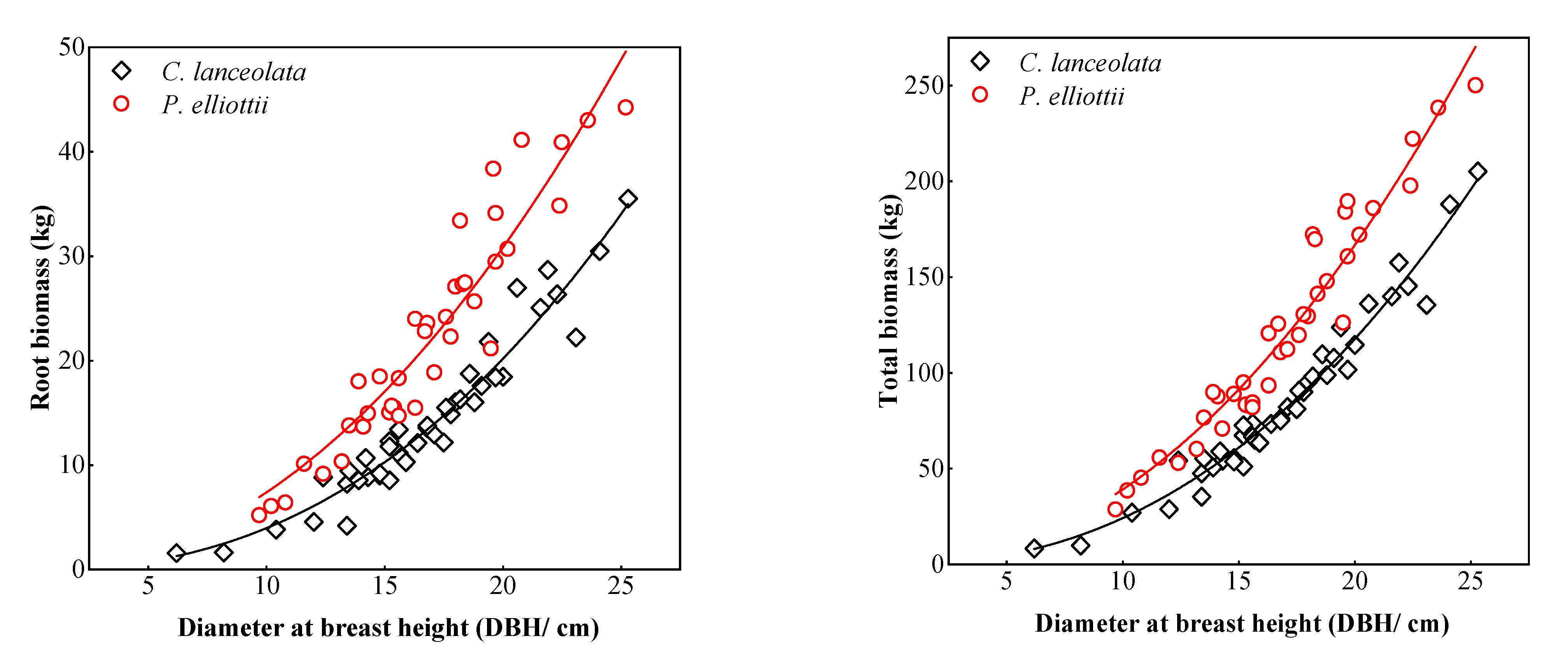
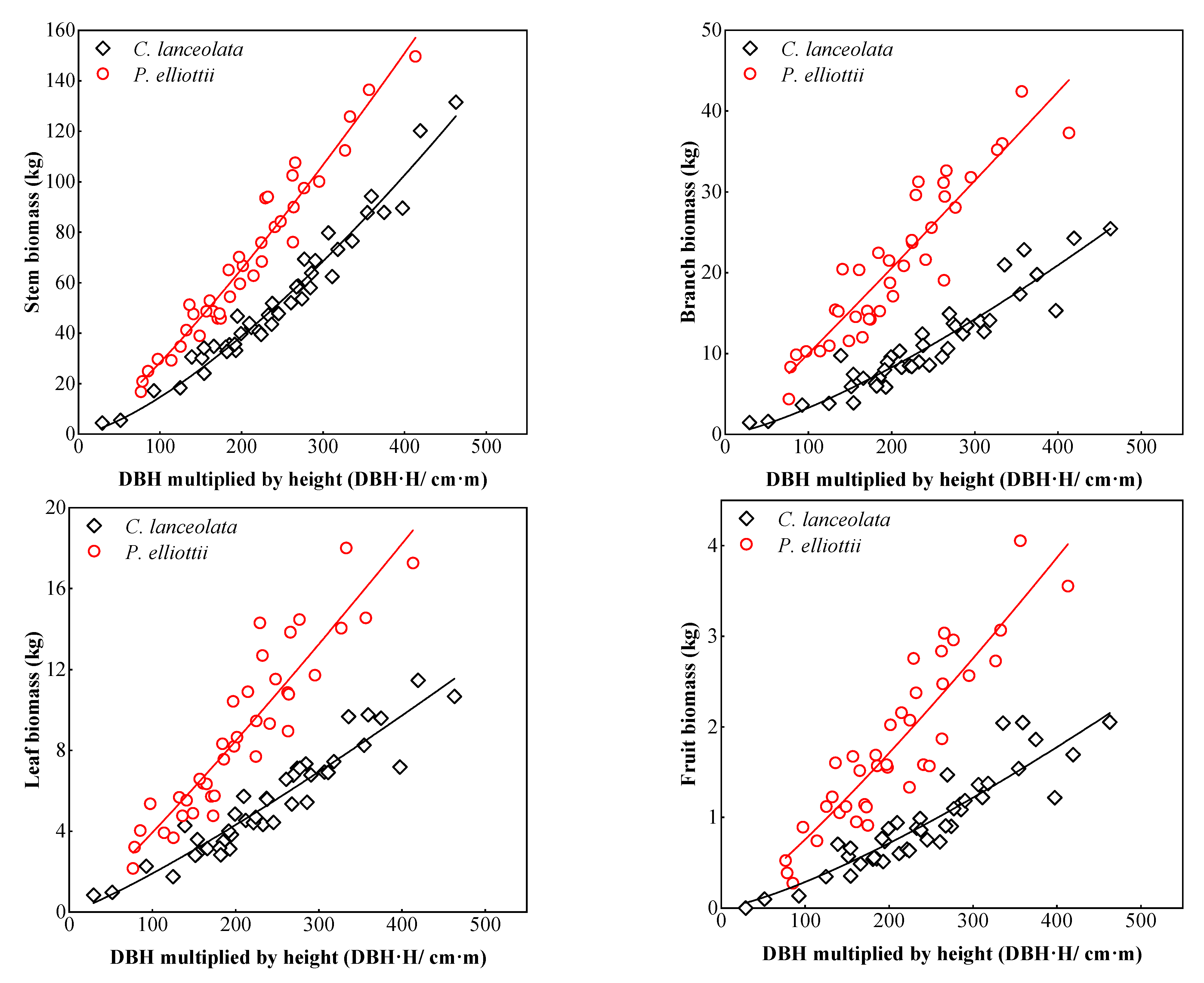
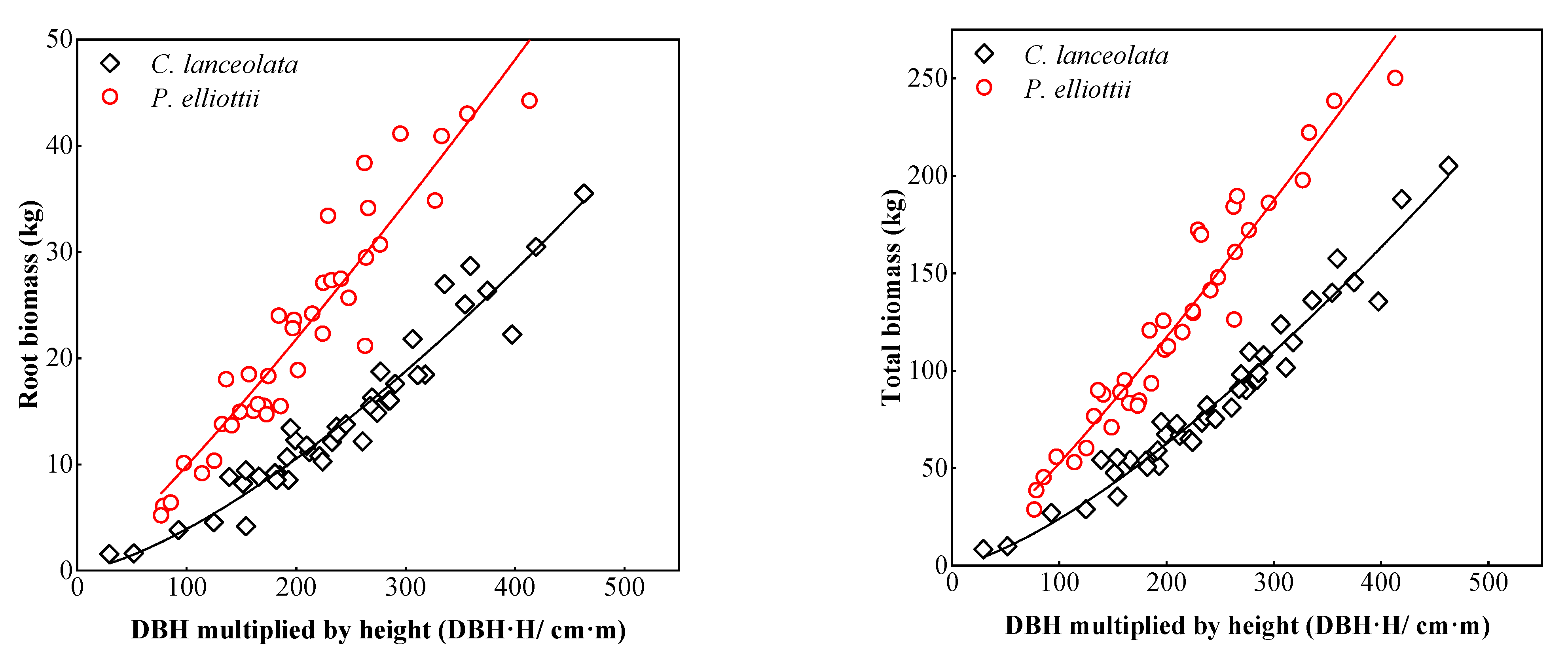
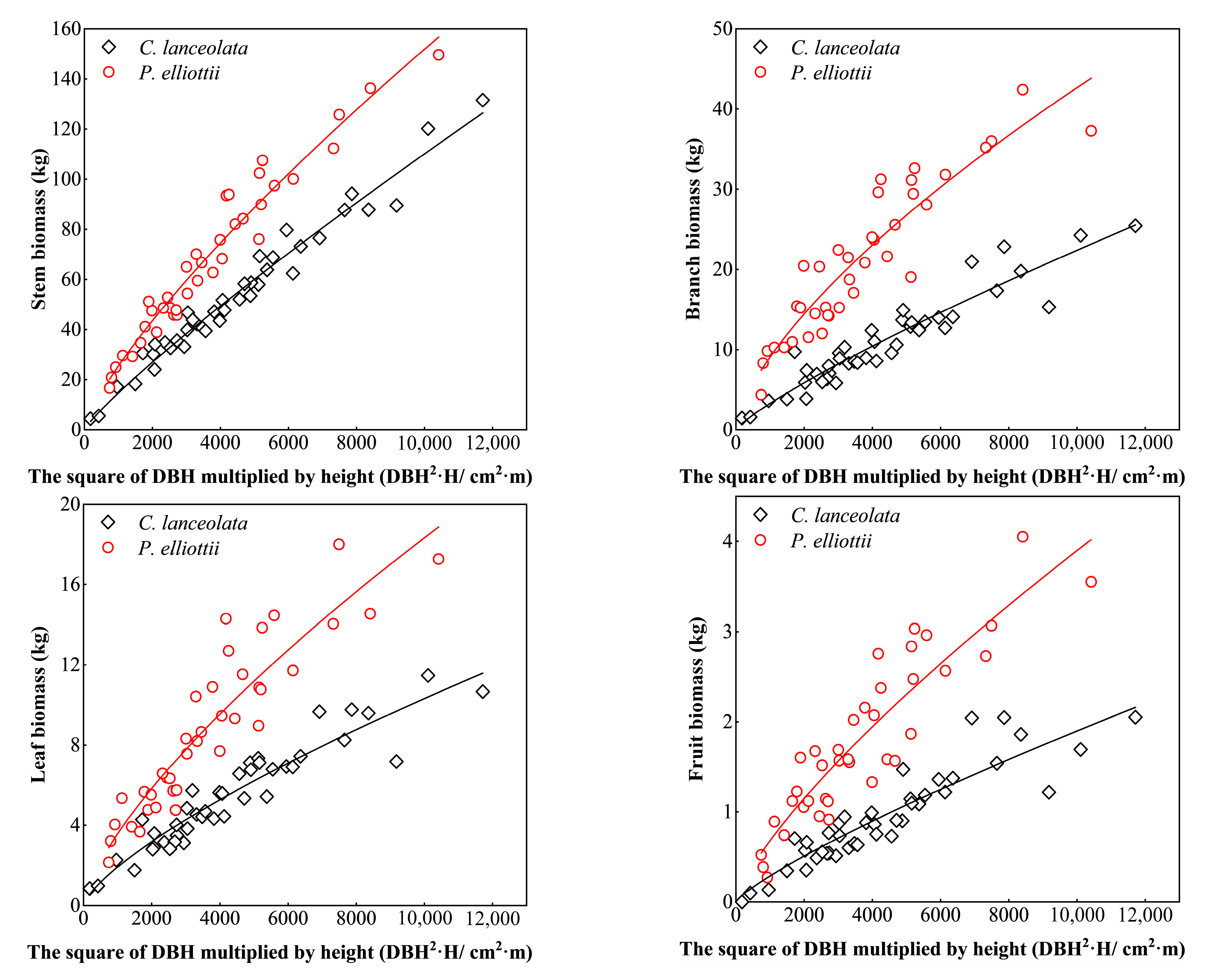
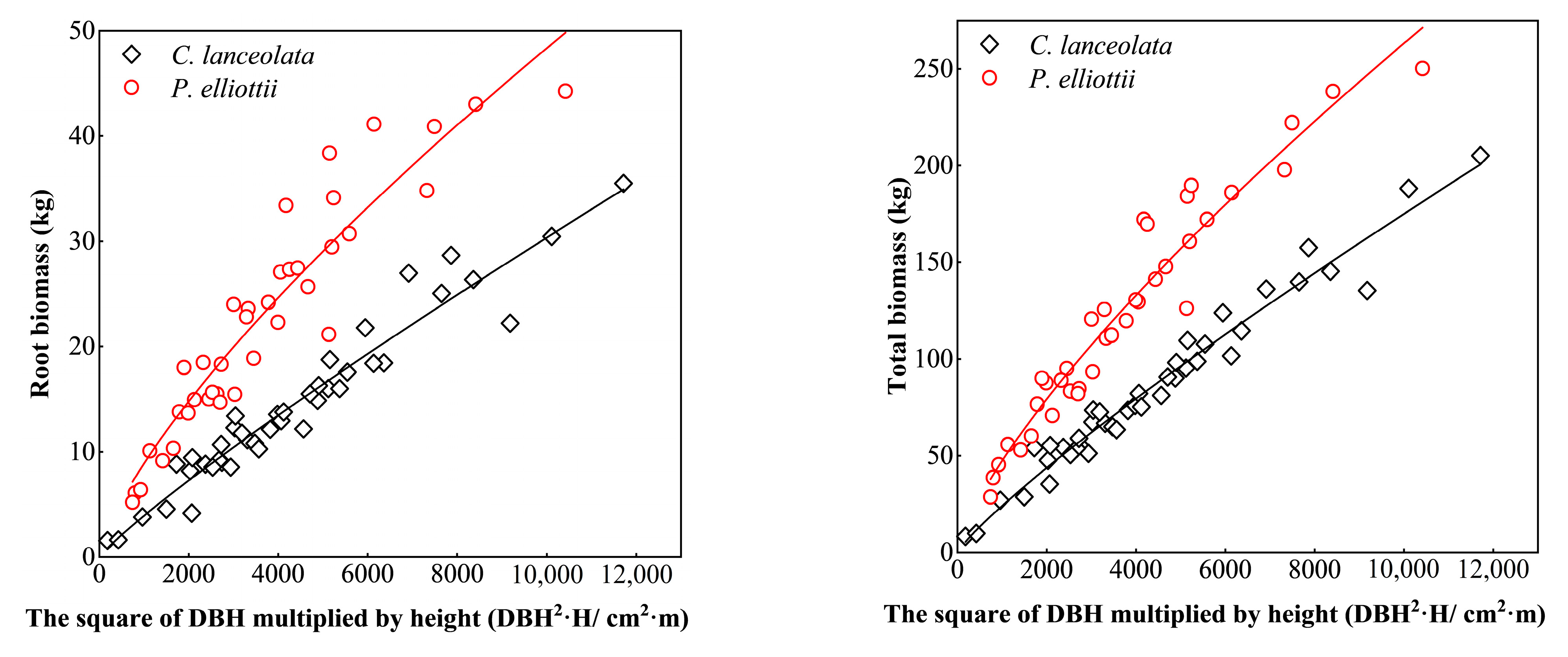
Biomass models of C. lanceolata and P. elliottii components were established with DBH and tree height as variables (Table 2, Figure 2, Figure 3 and Figure 4). There was a good power function relationship between the DBH and biomass of each component from C. lanceolata; R2 ranged from 0.832 to 0.971 (p < 0.05, n = 42). Similarly, the R2 of Equations (2) and (3) ranged from 0.836 to 0.964 and from 0.840 to 0.972, respectively. The R2 of the C. lanceolata biomass model constructed using Equation (3) was higher. There was also a good power function relationship between the DBH and biomass of each component from P. elliottii; R2 ranged from 0.836 to 0.951 (p < 0.05, n = 38). Similarly, the R2 of Equations (2) and (3) ranged from 0.825 to 0.951 and from 0.829 to 0.951, respectively. The R2 of the P. elliottii biomass model constructed using Equation (1) was higher. Therefore, we can measure the components’ biomass through these models and the DBH that has been measured, without cutting down the trees.

3.2. Forest Stand Biomass

3.2.1. Tree Layer Biomass

The biomass of the C. lanceolata tree layer was 94.7 t·ha−1 (Table 3), and the biomass and proportion of each component were as follows: stem (58.8 t·ha−1, 62.1%), root (16.0 t·ha−1, 16.9%), branch (12.4 t·ha−1, 13.1%), leaf (6.4 t·ha−1, 6.7%), fruit (1.1 t·ha−1, 1.1%). The biomass of the P. elliottii tree layer was 122.9 t·ha−1 (Table 3), and the biomass and proportion of each component were as follows: stem (68.2 t·ha−1, 55.5%), root (22.7 t·ha−1, 18.5%), branch (21.4 t·ha−1, 17.4%), leaf (8.8 t·ha−1, 7.2%), fruit (1.8 t·ha−1, 1.4%). There were significant differences in the total biomass or biomass of each component between the two coniferous forests (p < 0.05). The stem biomasses of the two coniferous forests were the highest among their respective components, but their proportions were different.

3.2.2. Understory Vegetation and Dead Cover Layer Biomass

The biomass and proportion of each component under the C. lanceolata forest were as follows: litter layer (9.4 t·ha−1, 42.0%), shrub (7.8 t·ha−1, 34.8%), herb (2.8 t·ha−1, 12.5%), dead wood (2.4 t·ha−1, 10.7%) (Table 4). The biomass and proportion of each component under the P. elliottii forest were as follows: litter layer (12.6 t·ha−1, 43.6%), shrub (9.9 t·ha−1, 34.3%), herb (3.5 t·ha−1, 12.1%), dead wood (2.9 t·ha−1, 10.0%) (Table 4). Only the litter layer and it’s the biomasses of the undecomposed layer showed significant differences between the two coniferous forests (p < 0.05), while others were not significantly different. Both deciduous coniferous forests had a relatively high litter layer biomass.

3.3. Carbon Concentration of Forest Ecosystem Components

3.3.1. Carbon Concentration in the Tree Layer

The carbon concentration of C. lanceolata components ranged from 46.9% to 51.4%, with the highest carbon concentration in leaves and the lowest in fruits (Table 5). Moreover, the carbon concentration of P. elliottii components ranged from 45.0% to 51.6%, with the highest carbon concentration in stems and the lowest in leaves (Table 5). The carbon concentrations of leaves, fruits and roots of C. lanceolata were significantly higher than those of P. elliottii. The results indicated that the carbon concentration of different tree species or different organs was different.

3.3.2. Carbon Concentration of the Understory Vegetation and Dead Cover Layer

In the C. lanceolata forest, the carbon concentrations of shrub, herb and dead wood were 49.8%, 43.3% and 49.2%, respectively, and that of litter ranged from 44.1% to 49.9% (Table 6). In the P. elliottii forest, the carbon concentrations of shrub, herb and dead wood were 49.9%, 43.6% and 50.5%, respectively, and that of litter ranged from 40.4% to 44.2% (Table 6). We found that the carbon concentration was lower in herb than in shrub, and in litter, it decreased with the increase in decomposition degree.

3.3.3. Soil Carbon Concentration

In the C. lanceolata forest, the SOC concentrations ranged from 4.3 to 17.5 g·kg−1 (Table 7), and gradually decreased with the increase in soil depth, and there were significant differences in SOC concentrations between different soil depths (p < 0.05). In the P. elliottii forest, the SOC concentrations ranged from 5.1 to 19.4 g·kg−1 (Table 7), and the characteristics were similar to those of the C. lanceolata forest. In addition, there were significant differences in SOC concentration between the two coniferous forests at the same soil depth (such as 0–20 and 20–40 cm). The BD of C. lanceolata and P. elliottii ranged from 1.21 to 1.46 g·cm−3 and 1.21 to 1.48 g·cm−3 (Table 7), respectively, and this increased with the increase in soil depth.

3.4. Carbon Density of Forest Ecosystem

3.4.1. Carbon Density in the Tree Layer

In the C. lanceolata forest, the carbon density of the tree layer was 47.5 t·ha−1 (Table 8), and the carbon density and proportion of each component were as follows: stem (29.8 t·ha−1, 62.7%), root (7.9 t·ha−1, 16.7%), branch (6.0 t·ha−1, 12.6%), leaf (3.3 t·ha−1, 6.9%), fruit (0.5 t·ha−1, 1.1%). In the P. elliottii forest, the carbon density of the tree layer was 60.8 t·ha−1 (Table 8), and the carbon density and proportion of each component were as follows: stem (35.2 t·ha−1, 57.9%), root (10.6 t·ha−1, 17.4%), branch (10.2 t·ha−1, 16.8%), leaf (4.0 t·ha−1, 6.5%), fruit (0.8 t·ha−1, 1.3%). There were significant differences in total carbon density or carbon density in each component between the two coniferous forests (p < 0.05), which was similar to the biomass.

3.4.2. Carbon Density in the Understory Vegetation and Dead Cover Layer

The carbon density and proportion of each component in the C. lanceolata forest were as follows: litter layer (4.4 t·ha−1, 41.1%), shrub (3.9 t·ha−1, 36.4%), herb (1.2 t·ha−1, 11.2%), dead wood (1.2 t·ha−1, 11.2%) (Table 9). The carbon density and proportion of each component in the P. elliottii forest were as follows: litter layer (5.4 t·ha−1, 40.6%), shrub (4.9 t·ha−1, 36.8%), herb (1.5 t·ha−1, 11.3%), dead wood (1.5 t·ha−1, 11.3%) (Table 9). Only the carbon density in undecomposed litter showed significant differences between the two coniferous forests (p < 0.05), while others did not. We found that carbon density decreased with the increase in decomposition in litter, which was similar to biomass.

3.4.3. Carbon Density in Soil

Overall, the soil carbon density was significantly higher in the P. elliottii forest than in the C. lanceolata forest at the same soil depth (Table 10). The total soil carbon density of C. lanceolata and P. elliottii were 108.1 t ha−1 and 124.6 t ha−1, respectively, and decreased significantly with the increase in soil depth (p < 0.05). In addition, about 70% of the total soil carbon was stored in the top 40 cm of the soil.

3.4.4. Total Carbon Density of Forest Ecosystem

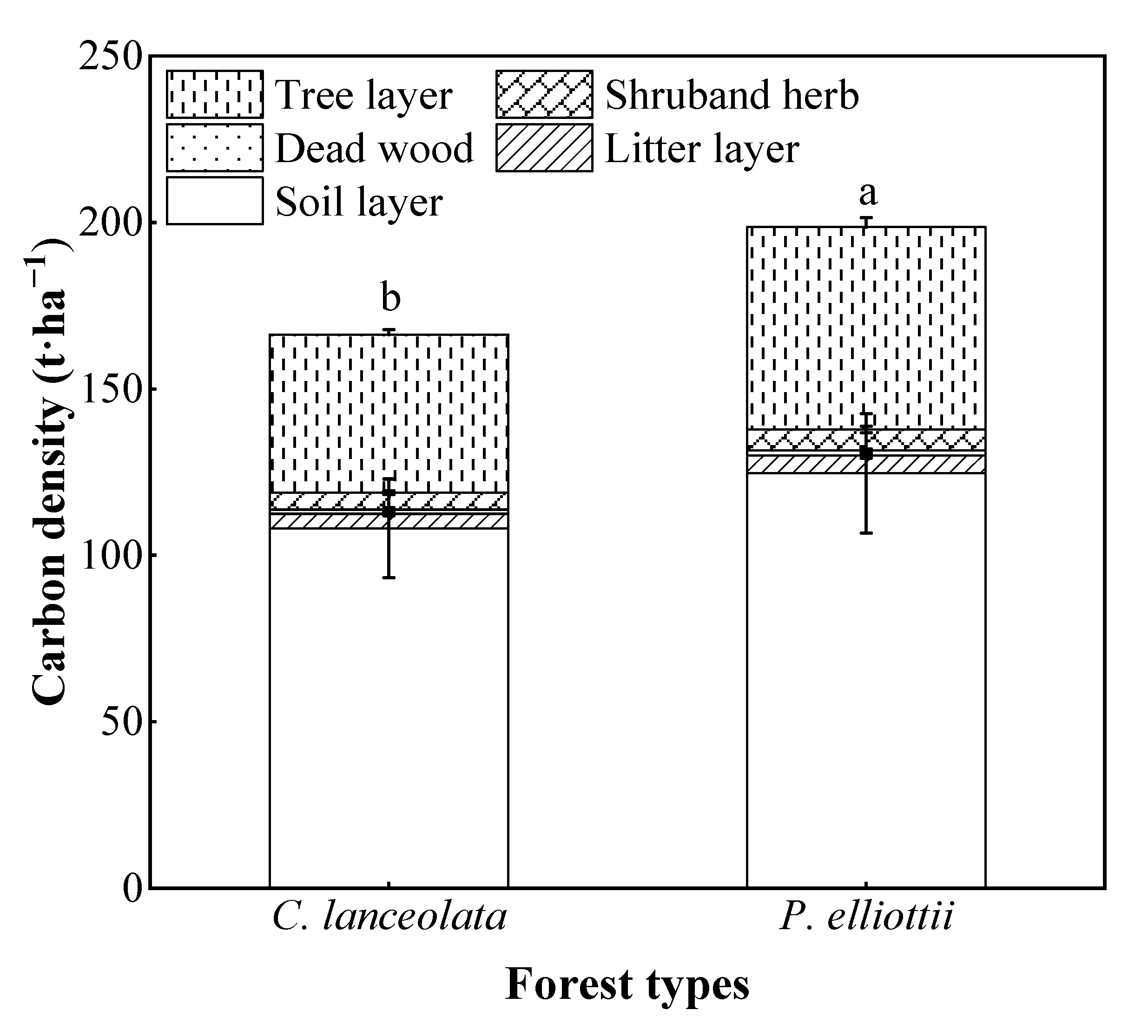
The total carbon density of C. lanceolata plantation ecosystem was 166.3 t·ha−1 (Figure 5), in which the soil carbon density accounted for 65.0% of the total, followed by the tree layer with a proportion of 28.6%, and then the shrub, herb, dead wood and litter with a cumulative proportion of 6.4%. The total carbon density of the P. elliottii plantation ecosystem was 198.6 t·ha−1 (Figure 5), in which the soil carbon density accounted for 62.7% of the total, followed by the tree layer with a proportion of 30.6%, and then the shrub, herb, dead wood and litter with a cumulative proportion of 6.7%. The total carbon density was significantly higher in the P. elliottii plantation ecosystem than in that of C. lanceolata (p < 0.05).

4. Discussion

4.1. Single Tree Biomass Model

Usually D, H, DH, D2H and V are used as variables to build a single tree biomass model (in which D represents the DBH, H represents the tree height and V represents the wood volume) [34,35,36,37]. In this study, the biomass models of two coniferous species were constructed with D, DH and D2H as variables, and all of them had results with a good fit. However, tree height is a variable that is difficult to measure accurately without felling trees in those plots. Therefore, the biomass of C. lanceolata and P. elliottii were estimated with only D as the variable, and R2 ranged from 0.832 to 0.971 and from 0.836 to 0.951, respectively (p < 0.05), which were still results with a good fit. This may be a good functional relationship between DBH and tree height or wood volume itself, and DBH is sufficient to reflect the growth status and biomass of individual trees [36,38]. In addition, with the support of the National Fund, more sample trees will be harvested to improve these models.

4.2. Biomass and Distribution in Plantations

Biomass and its distribution in artificial forests is related to many factors such as water, temperature, soil fertility, tree age, planting density, tree species composition and management mode [30,39,40,41]. In this study, C. lanceolata and P. elliottii, with the same age of 19 years, had a different tree layer biomass, and although the planting density of P. elliottii was smaller, it did have higher biomass. This indicates that the effect of tree species on forest biomass is obvious, which has been similarly reported in previous studies [42,43,44]. The biomass in each component of the two coniferous forests had the following order: stem > root > branch > leaf > fruit, which was similar to the results of previous studies; however, the percentage of each component’s biomass to total biomass was different [42,45].
The composition and growth of understory vegetation are affected by many factors such as forest type, planting density and site conditions. The biomass of shrubs and herbs is mainly determined by the biological characteristics of the plant itself and is also affected by environmental factors such as light and nutrients [42]. In addition, there was a significant negative correlation between the understory biomass and canopy density [42]. In this study, there were differences in undergrowth vegetation type between the two coniferous forests (Table 1), and the biomass of shrubs and herbs was lower in the C. lanceolata forest (5.1 t·ha−1), with a higher planting density and canopy closure than in the P. elliottii forest (6.3 t·ha−1).
Dead wood is named coarse woody debris (CWD) with a diameter of >10 cm and a length of >1 m in the forest. It affects the energy flow, nutrient cycle and carbon storage in the forest ecosystem, and plays a role in regulating the forest microclimate, conserving soil and water, promoting soil development, and protecting forest ecosystem diversity [46,47]. However, dead wood was an easily overlooked part of previous forest biomass research. In this study, the dead wood biomass of C. lanceolata and P. elliottii plantations were 2.4 t·ha−1 and 2.9 t·ha−1, accounting for 2.0% and 1.9% of their total biomass, respectively.
The litter layer plays an important role in connecting the forest and soil, improving soil structure and reducing soil erosion. At the same time, the nutrients released by litter decomposition also promote plants’ growth, and the biomass and decomposition rate of litter were related to a plant’s biological characteristics, stand structure and accumulation years [48,49,50]. In this study, the litter biomass in the C. lanceolata forest was 9.4 t·ha−1, in which the biomass of the undecomposed layer was 3.8 t·ha−1, which was significantly higher than that of a 15-year-old C. lanceolata in Huitong [30]. The litter biomass in the P. elliottii forest was 12.6 t·ha−1, in which the biomass of undecomposed layer was 6.6 t·ha−1, which was significantly higher than that of the C. lanceolata at a same age. The reason may be due to the biological differences between the two conifer species themselves.

4.3. Forest Carbon Concentration

Carbon concentration is a necessary parameter to estimate the carbon storage of forest ecosystems. Previous studies have shown that some scholars often use the international general carbon conversion coefficient of 0.5, which can reduce the difficulty of work in large-scale research [51,52]. However, the carbon concentrations are measured using plant samples, because that of tree species and their components are different. The carbon concentration in C. lanceolata was found to be as follows: 47.7%–53.6% (with trees aged 15 year old and with 2000 trees per ha−1, in Huitong) [30], 48.2%–52.0% [53], 45.8%–50.9% (with trees aged 14 years old and with 2400 trees per ha−1, in Changsha) [45] and 46.9%–51.4% in this study. The carbon concentration in P. elliottii was found to be as follows: 43.2%–51.9% (with trees aged 22 years old and with 1400 trees per ha−1, in Qianyanzhou) [54], 44.4%–46.6% (with trees aged 20 years old and 950 trees per ha−1, in Guizhou) [55], 48.0%–51.0% (with trees aged 30 years old and 1500 trees per ha−1, on Pingtan Island) [56], and 45.0%–51.6% in this study. Although the results of the above studies are similar, there are still differences.

4.4. Forest Carbon Density and Its Distribution

The total carbon density of the C. lanceolata forest in this study was 166.3 t·ha−1, higher than the 123.1 t·ha−1 in Huitong [30], 104.1 t·ha−1 in Hengyang (with trees aged 14 years old and 1230 trees per ha−1) [33], but lower than the 176.7 t·ha−1 in Changsha [45] and 167.7 t·ha−1 in Guangzhou (with trees aged 19 years old and 1200 trees per ha−1) [57]. In addition, the carbon density of P. elliottii was 198.6 t·ha−1, higher than the 103.9 t·ha−1 in Taihe (with trees aged 19 years old and 633 trees per ha−1) [58], 116.8 t·ha−1 in Qianyanzhou [54], 113.9–173.7 t·ha−1 in Florida (with trees aged 17 years old and 1530–1790 trees per ha−1) [59], but lower than the 834.1 t·ha−1 (in which soil carbon density was 756.9 t·ha−1) in Guizhou [55]. The above studies indicate that the carbon density of C. lanceolata or P. elliottii from different regions is different, which may be related to the climate, planting density, tree age, soil conditions and other factors in the study area. However, the distribution characteristics of carbon density in forests in different region showed consistency, namely soil > vegetation > litter.
Soil is the principal part of forest carbon storage. In this study, soil carbon storage accounted for 62.7–65.0% of the whole ecosystem, which was similar to C. lanceolata (66.2%) and Pinus massoniana (64.5%) in Changsha [45], slightly higher than P. elliottii (60.3%) and lower than C. lanceolata (70.4%) in Hengyang [33], higher than C. lanceolata (55.2%) in Huitong [30], and far lower than P. elliottii (90.7%) in Guizhou [55]. Soil carbon storage is related to the thickness and carbon content of the soil itself, and its proportion in the whole ecosystem is also related to vegetation carbon storage. Litter decomposition, soil fauna and microorganisms together increase the soil carbon concentration.

5. Conclusions

Through the power function equation (Equations (1)–(3)), the biomass models of the whole tree or each component of two coniferous species were established (Table 2), and R2 ranged from 0.825 to 0.971. Based on the DBH of each tree in the plot, the biomass of C. lanceolata and P. elliottii plantations were estimated to be 94.7 t·ha−1 and 122.9 t·ha−1, respectively, which indicates that the net productivity of P. elliottii is higher. The components’ biomass in C. lanceolata and P. elliottii forests were as follows: understory vegetation: 10.6 and 13.4 t·ha−1; dead wood: 2.4 and 2.9 t·ha−1; and litter: 9.4 and 12.6 t·ha−1, respectively, which indicates that the biomass yield of the P. elliottii forest ecosystem is higher. The carbon concentration in the two coniferous forests was as follows: vegetation: 43.3%–51.6%; litter and dead wood: 40.4%–50.5%; and soil: 4.3–19.4 g·kg−1. The ecosystem carbon density of C. lanceolata and P. elliottii was 166.3 and 198.6 t·ha−1, and the proportion of soil was 65.0% and 62.7%, respectively. This indicates that the carbon sink capacity of the P. elliottii plantation is higher. The differences in the biological characteristics of the two coniferous forests lead to differences in their biomass and carbon storage capacity with the same tree age and site conditions. The faster regeneration of branches and leaves in the P. elliottii forest results in the higher carbon storage of litter and soil. Both coniferous forests are fast-growing and high-yield species, which are of great significance in improving forest carbon sink capacity and mitigating negative climate changes.

Author Contributions

Research ideas and methods, H.L., J.C. and J.H.; experiments and data analysis, H.L. and J.C.; visualization, H.L. and J.C.; writing—original draft preparation, H.L.; writing—review and editing, J.H. and W.K.; fund management, J.L. (Jianjun Li) and J.L. (Jianan Li). All authors have read and agreed to the published version of the manuscript.

Funding

This study (including the APC) was supported by the National Key Research and Development Project: forest site quality evaluation and full-cycle multifunctional management decision platform (2022YFD2200505).

Institutional Review Board Statement

This study does not involve humans and animals.

Informed Consent Statement

This study does not involve humans and animals.

Data Availability Statement

The datasets of this study are available from the corresponding author.

Acknowledgments

We thank the other workers who helped this research, from the Central South University of Forestry and Technology, Shengfeng and Tashi state-owned forest farms.

Conflicts of Interest

The authors declare no conflict of interest.

References

  1. Robinson, R.A.; Crick, H.Q.P.; Learmonth, J.A.; Maclean, I.M.D.; Thomas, C.D.; Bairlein, F.; Forchhammer, M.C.; Francis, C.M.; Gill, J.A.; Godley, B.J.; et al. Travelling through a warming world: Climate change and migratory species. Endanger. Species Res. 2009, 7, 87–99. [Google Scholar] [CrossRef]
  2. McMichael, A.J.; Woodruff, R.E.; Hales, S. Climate change and human health: Present and future risks. Lancet 2006, 367, 859–869. [Google Scholar] [CrossRef] [PubMed]
  3. Pecl, G.T.; Araújo, M.B.; Bell, J.D.; Blanchard, J.; Bonebrake, T.C.; Chen, I.C.; Clark, T.D.; Colwell, R.K.; Danielsen, F.; Evengård, B.; et al. Biodiversity redistribution under climate change: Impacts on ecosystems and human well-being. Science 2017, 355, eaai9214. [Google Scholar] [CrossRef]
  4. Pan, Y.; Birdsey, R.A.; Fang, J.; Houghton, R.; Kauppi, P.E.; Kurz, W.A.; Phillips, O.L.; Shvidenko, A.; Lewis, S.L.; Canadell, J.G.; et al. A large and persistent carbon sink in the world’s forests. Science 2011, 333, 988–993. [Google Scholar] [CrossRef] [Green Version]
  5. Gren, I.M.; Zeleke, A.A. Policy design for forest carbon sequestration: A review of the literature. For. Policy Econ. 2016, 70, 128–136. [Google Scholar] [CrossRef] [Green Version]
  6. Brinck, K.; Fischer, R.; Groeneveld, J.; Lehmann, S.; Dantas De Paula, M.; Pütz, S.; Sexton, J.O.; Song, D.; Huth, A. High resolution analysis of tropical forest fragmentation and its impact on the global carbon cycle. Nat. Commun. 2017, 8, 14855. [Google Scholar] [CrossRef] [PubMed] [Green Version]
  7. Bernal, B.; Murray, L.T.; Pearson, T.R.H. Global carbon dioxide removal rates from forest landscape restoration activities. Carbon Balance Manag. 2018, 13, 22. [Google Scholar] [CrossRef]
  8. Heinonen, T.; Pukkala, T.; Mehtätalo, L.; Asikainen, A.; Kangas, J.; Peltola, H. Scenario analyses for the effects of harvesting intensity on development of forest resources, timber supply, carbon balance and biodiversity of Finnish forestry. For. Policy Econ. 2017, 80, 80–98. [Google Scholar] [CrossRef] [Green Version]
  9. Gough, C.M.; Vogel, C.S.; Harrold, K.H.; George, K.; Curtis, P.S. The legacy of harvest and fire on ecosystem carbon storage in a north temperate forest. Glob. Chang. Biol. 2007, 13, 1935–1949. [Google Scholar] [CrossRef]
  10. Li, X.; Li, Y.; Chen, A.; Gao, M.; Slette, I.J.; Piao, S. The impact of the 2009/2010 drought on vegetation growth and terrestrial carbon balance in Southwest China. Agric. For. Meteorol. 2019, 269, 239–248. [Google Scholar] [CrossRef]
  11. Zhang, Y.; Zhou, X.; Qin, Q.; Chen, K. Value accounting of forest carbon sinks in China. J. Beijing For. Univ. 2013, 35, 124–131. [Google Scholar] [CrossRef]
  12. IGBP Terrestrial Carbon Working Group. The terrestrial carbon cycle: Implications for the Kyoto Protocol. Science 1998, 280, 1393–1394. [Google Scholar] [CrossRef] [Green Version]
  13. Ma, X.; Xiong, K.; Zhang, Y.; Lai, J.; Zhang, S.; Ji, C. Research progresses and prospects of carbon storage in forest ecosystems. J. Northwest For. Univ. 2019, 34, 62–72. [Google Scholar] [CrossRef]
  14. Sun, W.; Liu, X. Review on carbon storage estimation of forest ecosystem and applications in China. For. Ecosyst. 2020, 7, 4. [Google Scholar] [CrossRef] [Green Version]
  15. Fang, J.; Chen, A.; Peng, C.; Zhao, S.; Ci, L. Changes in forest biomass carbon storage in China between 1949 and 1998. Science 2001, 292, 2320–2322. [Google Scholar] [CrossRef]
  16. Schwendenmann, L.; Pendall, E. Effects of forest conversion into grassland on soil aggregate structure and carbon storage in Panama: Evidence from soil carbon fractionation and stable isotopes. Plant Soil 2006, 288, 217–232. [Google Scholar] [CrossRef]
  17. Luo, X.; Hou, E.; Zhang, L.; Wen, D. Soil carbon dynamics in different types of subtropical forests as determined by density fractionation and stable isotope analysis. For. Ecol. Manag. 2020, 475, 118401. [Google Scholar] [CrossRef]
  18. Goetz, S.; Dubayah, R. Advances in remote sensing technology and implications for measuring and monitoring forest carbon stocks and change. Carbon Manag. 2011, 2, 231–244. [Google Scholar] [CrossRef]
  19. Zhao, J.; Xie, H.; Ma, J.; Wang, K. Integrated remote sensing and model approach for impact assessment of future climate change on the carbon budget of global forest ecosystems. Glob. Planet. Chang. 2021, 203, 103542. [Google Scholar] [CrossRef]
  20. Zhang, Y.; Li, X.; Wen, Y. Forest carbon sequestration potential in China under the background of carbon emission peak and carbon neutralization. J. Beijing For. Univ. 2022, 44, 38–47. [Google Scholar] [CrossRef]
  21. Qiu, Z.; Feng, Z.; Song, Y.; Li, M.; Zhang, P. Carbon sequestration potential of forest vegetation in China from 2003 to 2050: Predicting forest vegetation growth based on climate and the environment. J. Clean. Prod. 2020, 252, 119715. [Google Scholar] [CrossRef]
  22. Payn, T.; Carnus, J.M.; Freer-Smith, P.; Kimberley, M.; Kollert, W.; Liu, S.; Orazio, C.; Rodriguez, L.; Silva, L.N.; Wingfield, M.J. Changes in planted forests and future global implications. For. Ecol. Manag. 2015, 352, 57–67. [Google Scholar] [CrossRef] [Green Version]
  23. Mei, M.; Lei, Y. Analysis on development trend of China’s plantation in new era. World For. Res. 2019, 32, 73–77. [Google Scholar] [CrossRef]
  24. Liu, S.; Yang, Y.; Wang, H. Development strategy and management countermeasures of planted forests in China: Transforming from timber-centered single objective management towards multi-purpose management for enhancing quality and benefits of ecosystem services. Acta Ecol. Sin. 2018, 38, 1–10. [Google Scholar] [CrossRef]
  25. Zhang, H.; Zhou, G.; Wang, Y.; Bai, S.; Sun, Z.; Berninger, F.; Bai, Y.; Penttinen, P. Thinning and species mixing in Chinese fir monocultures improve carbon sequestration in subtropical China. Eur. J. For. Res. 2019, 138, 433–443. [Google Scholar] [CrossRef]
  26. Bracho, R.; Starr, G.; Gholz, H.L.; Martin, T.A.; Cropper, W.P.; Loescher, H.W. Controls on carbon dynamics by ecosystem structure and climate for southeastern US slash pine plantations. Ecol. Monogr. 2012, 82, 101–128. [Google Scholar] [CrossRef]
  27. Zeng, W. Development of Volume-derived Biomass Models for Three Coniferous Forest Types in China. For. Res. 2021, 34, 49–57. [Google Scholar] [CrossRef]
  28. Wang, L.; Zhang, Y.; Berninger, F.; Duan, B. Net primary production of Chinese fir plantation ecosystems and its relationship to climate. Biogeosciences 2014, 11, 5595–5606. [Google Scholar] [CrossRef] [Green Version]
  29. Cai, H.; Di, X.; Chang, S.X.; Wang, C.; Shi, B.; Geng, P.; Jin, G. Carbon storage, net primary production, and net ecosystem production in four major temperate forest types in northeastern China. Can. J. For. Res. 2016, 46, 143–151. [Google Scholar] [CrossRef]
  30. Wang, Q.; Wang, S.; Zhang, J. Assessing the effects of vegetation types on carbon storage fifteen years after reforestation on a Chinese fir site. For. Ecol. Manag. 2009, 258, 1437–1441. [Google Scholar] [CrossRef]
  31. He, Y.; Qin, L.; Li, Z.; Liang, X.; Shao, M.; Tan, L. Carbon storage capacity of monoculture and mixed-species plantations in subtropical China. For. Ecol. Manag. 2013, 295, 193–198. [Google Scholar] [CrossRef]
  32. Qin, L.; He, Y.; Li, Z.; Shao, M.; Liang, X.; Tan, L. Allocation pattern of biomass and productivity for three plantations of Castanopsis hystrix, Pinus massoniana and their mixture in south subtropical area of Guangxi, China. Sci. Silvae Sin. 2011, 47, 17–21. [Google Scholar]
  33. Zheng, H.; Ouyang, Z.; Xu, W.; Wang, X.; Miao, H.; Li, X.; Tian, Y. Variation of carbon storage by different reforestation types in the hilly red soil region of southern China. For. Ecol. Manag. 2008, 255, 1113–1121. [Google Scholar] [CrossRef]
  34. Zhao, J.; Li, H. Establishment of below-ground biomass equations for Chinese fir at tree and stand level. Sci. Silvae Sin. 2018, 54, 81–89. [Google Scholar] [CrossRef]
  35. Zhang, X.; Duan, A.; Zhang, J. Tree biomass estimation of Chinese fir (Cunninghamia lanceolata) based on Bayesian method. PLoS ONE 2013, 8, e79868. [Google Scholar] [CrossRef] [PubMed] [Green Version]
  36. Mei, G.; Sun, Y.; Sajjad, S. Models for predicting the biomass of Cunninghamia lanceolata trees and stands in Southeastern China. PLoS ONE 2017, 12, e0169747. [Google Scholar] [CrossRef] [Green Version]
  37. Zhao, D.; Westfall, J.; Coulston, J.W.; Lynch, T.B.; Bullock, B.P.; Montes, C.R. Additive biomass equations for slash pine trees: Comparing three modeling approaches. Can. J. For. Res. 2019, 49, 27–40. [Google Scholar] [CrossRef]
  38. Li, Y.; Zhang, J.; Duan, A.; Xiang, C. Selection of biomass estimation models for Chinese fir plantation. Chin. J. Appl. Ecol. 2010, 21, 3036–3046. [Google Scholar] [CrossRef]
  39. Wang, Z.; Zhang, X.; Chhin, S.; Zhang, J.; Duan, A. Disentangling the effects of stand and climatic variables on forest productivity of Chinese fir plantations in subtropical China using a random forest algorithm. Agric. For. Meteorol. 2021, 304, 108412. [Google Scholar] [CrossRef]
  40. Huang, Z.; He, Z.; Wan, X.; Hu, Z.; Fan, S.; Yang, Y. Harvest residue management effects on tree growth and ecosystem carbon in a Chinese fir plantation in subtropical China. Plant Soil 2013, 364, 303–314. [Google Scholar] [CrossRef]
  41. Cobb, W.R.; Will, R.E.; Daniels, R.F.; Jacobson, M.A. Aboveground biomass and nitrogen in four short-rotation woody crop species growing with different water and nutrient availabilities. For. Ecol. Manag. 2008, 255, 4032–4039. [Google Scholar] [CrossRef]
  42. Guo, S.; Zhao, H.; Zhou, G.; Long, W.; Gan, G.; Wu, S.; Meng, M.; Chen, J. Biomass and Its Distribution Pattern of Four Tree Species Plantation in South Subtropical China. For. Res. 2022, 35, 182–189. [Google Scholar] [CrossRef]
  43. Dong, L.; Zhang, L.; Li, F. Developing two additive biomass equations for three coniferous plantation species in Northeast China. Forests 2016, 7, 136. [Google Scholar] [CrossRef] [Green Version]
  44. Labrecque, M.; Teodorescu, T.I. Field performance and biomass production of 12 willow and poplar clones in short-rotation coppice in southern Quebec (Canada). Biomass Bioenergy 2005, 29, 1–9. [Google Scholar] [CrossRef]
  45. Yu, R.; Xiang, W.; Ning, C.; Luo, Z. Carbon storage and sequestration in four urban forest ecosystems in Changsha, Hunan. Acta Ecol. Sin 2016, 36, 3499–3509. [Google Scholar]
  46. Bunnell, F.L.; Houde, I. Down wood and biodiversity—Implications to forest practices. Environ. Rev. 2010, 18, 397–421. [Google Scholar] [CrossRef]
  47. Wang, Y.; Chen, X.; Zou, D.; Lei, J.; Wu, X.; Wang, J.; Yan, W.; Liang, X. Biomass, carbon storage and nutrient content of coarse woody debris in secondary-growth forests in southern Hunan. Acta Ecol. Sin. 2022, 42, 3441–3448. [Google Scholar] [CrossRef]
  48. Krishna, M.P.; Mohan, M. Litter decomposition in forest ecosystems: A review. Energy Ecol. Environ. 2017, 2, 236–249. [Google Scholar] [CrossRef]
  49. Santonja, M.; Fernandez, C.; Proffit, M.; Gers, C.; Gauquelin, T.; Reiter, I.M.; Cramer, W.; Baldy, V. Plant litter mixture partly mitigates the negative effects of extended drought on soil biota and litter decomposition in a Mediterranean oak forest. J. Ecol. 2017, 105, 801–815. [Google Scholar] [CrossRef] [Green Version]
  50. Oliveira, R.A.C.; Marques, R.; Marques, M.C.M. Plant diversity and local environmental conditions indirectly affect litter decomposition in a tropical forest. Appl. Soil Ecol. 2019, 134, 45–53. [Google Scholar] [CrossRef]
  51. Houghton, R.A.; Skole, D.L.; Nobre, C.A.; Hackler, J.L.; Lawrence, K.T.; Chomentowski, W.H. Annual fluxes of carbon from deforestation and regrowth in the Brazilian Amazon. Nature 2000, 403, 301–304. [Google Scholar] [CrossRef]
  52. Liu, X.; Xu, X.; Hong, A. Study on forest carbon storage and carbon density in Hefei City. J. Soil Water Conserv. 2011, 25, 192–196. [Google Scholar] [CrossRef]
  53. Chen, L.; Guan, X.; Li, H.; Wang, Q.; Zhang, W.; Yang, Q.; Wang, S. Spatiotemporal patterns of carbon storage in forest ecosystems in Hunan Province, China. For. Ecol. Manag. 2019, 432, 656–666. [Google Scholar] [CrossRef]
  54. Ma, Z.; Hartmann, H.; Wang, H.; Li, Q.; Wang, Y.; Li, S. Carbon dynamics and stability between native Masson pine and exotic slash pine plantations in subtropical China. Eur. J. For. Res. 2014, 133, 307–321. [Google Scholar] [CrossRef]
  55. Liu, Z.; Ning, C.; Yan, W.; Ni, X.; Chen, Y.; Ning, X. Three kinds of pine forest biomass and carbon storage research in karst landform. J. Cent. South Univ. For. Technol. 2017, 37, 105–111. [Google Scholar] [CrossRef]
  56. Zhong, C.; Huang, Y.; Zhang, Q.; Wen, H. The stoichiometric characteristics and carbon, nitrogen stores of four main coastal shelterbelt forests in Pingtan. J. Southwest For. Univ. 2016, 36, 96–102. [Google Scholar]
  57. Lin, W.; Li, J.; Zhou, P.; Wei, L. Spatial distribution of carbon storage of three forests ecosystem in Guangzhou, China. For. Environ. Sci. 2014, 30, 1–7. [Google Scholar]
  58. Wei, X.; Li, Q.; Liu, Y.; Liu, S.; Guo, X.; Zhang, L.; Niu, D. Restoring ecosystem carbon sequestration through afforestation: A sub-tropic restoration case study. For. Ecol. Manag. 2013, 300, 60–67. [Google Scholar] [CrossRef]
  59. Shan, J.; Morris, L.A.; Hendrick, R.L. The effects of management on soil and plant carbon sequestration in slash pine plantations. J. Appl. Ecol. 2001, 38, 932–941. [Google Scholar] [CrossRef]
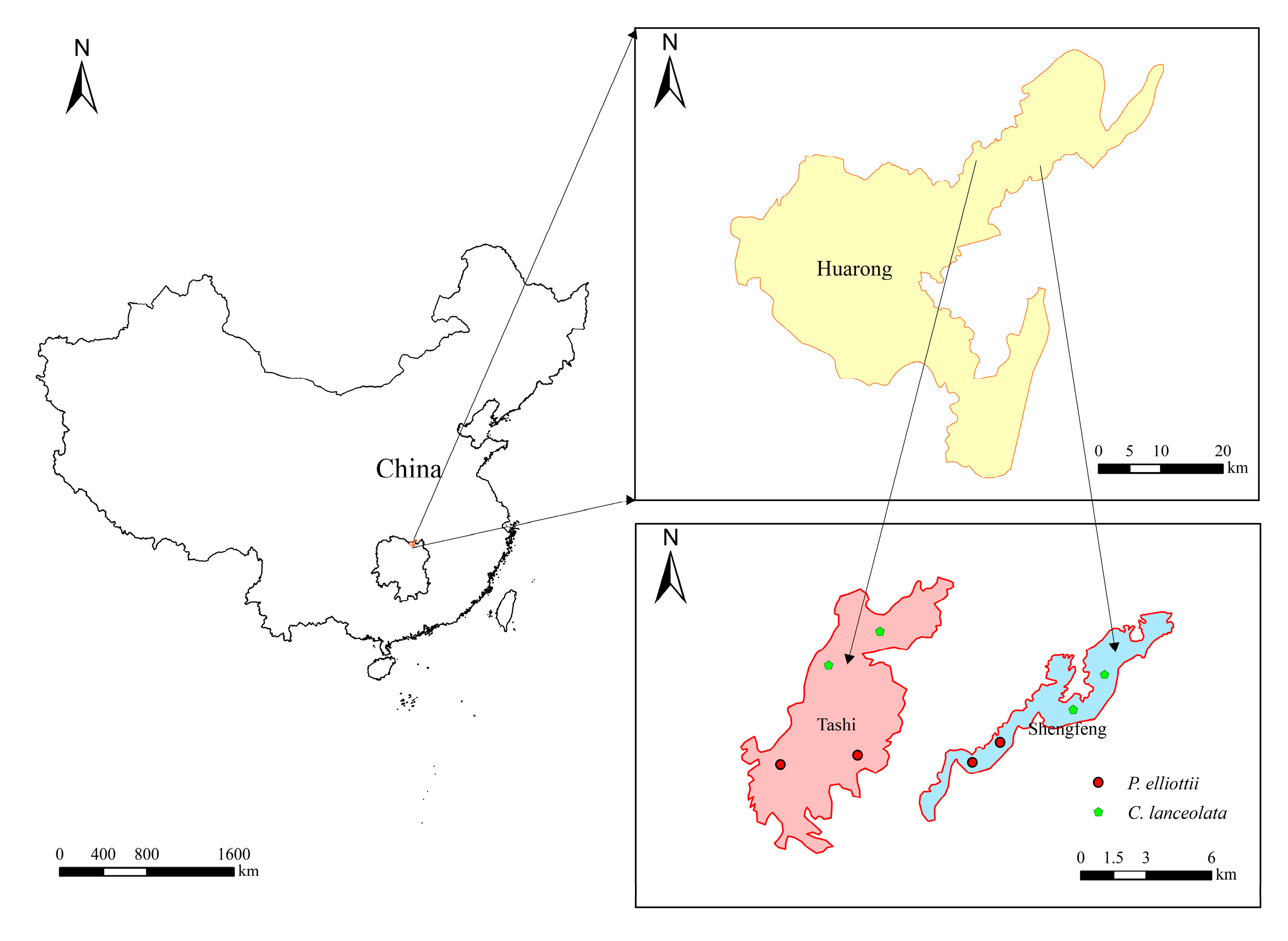
Figure 1. The plot location of C. lanceolata and P. elliottii in Huarong County.
Forests 14 00814 g001
Figure 2. The power function curves of biomass and DBH of C. lanceolata and P. elliottii components. n = 42 in C. lanceolata forest, n = 38 in P. elliottii forest.
Forests 14 00814 g002aForests 14 00814 g002b
Figure 3. The power function curves of biomass and the product (DBH multiplied by height) from C. lanceolata and P. elliottii components. n = 42 in C. lanceolata forest, n = 38 in P. elliottii forest.
Forests 14 00814 g003aForests 14 00814 g003b
Figure 4. The power function curves of biomass and the product (square of DBH multiplied by height) from C. lanceolata and P. elliottii components. n = 42 in C. lanceolata forest, n = 38 in P. elliottii forest.
Forests 14 00814 g004aForests 14 00814 g004b
Figure 5. The total carbon density and distribution of the C. lanceolata and P. elliottii plantation ecosystems. Vertical lines denote standard deviations, followed by the different lowercase letters which represent significant difference in total carbon density between the two coniferous forests at p < 0.05 level.
Forests 14 00814 g005
Table 1. Stand characteristics of C. lanceolata and P. elliottii plots.
ParameterForest Type
C. lanceolataP. elliottii
Age1919
Stand density1363 (43)1088 (25)
Average DBH/cm15.6 (2.8)16.3 (2.7)
Soil bulk density/g·cm−31.34 (0.11)1.36 (0.12)
Soil pH4.60 (0.20)4.60 (0.26)
Soil organic carbon/g·kg−110.4 (5.3)11.8 (6.0)
Total nitrogen/g·kg−11.24 (0.47)1.31 (0.53)
Total phosphorus/g·kg−10.32 (0.14)0.33 (0.13)
Total kalium/g·kg−15.14 (1.94)5.72 (2.51)
Sand (>0.02 mm):Silt (0.002–0.02 mm):Clay (<0.002 mm)/(%:%:%)40.5:38.1:21.444.6:35.9:19.5
Forest management measureIn 2019, the thinning intensity was 20%–30%In 2018, the thinning intensity was 20%–30%
Main understory plantsDicranopteris dichotoma
Camellia sinensis
Symplocos sumuntia
Lygodium japonicum
Loropetalum chinense
Symplocos sumuntia
Dicranopteris dichotoma
Macleaya cordata
Data are means followed by standard deviations in the parentheses. The soil depth was 0–80 cm.
Table 2. Biomass model parameters of C. lanceolata and P. elliottii.
EquationForest TypeComponentsModel ParametersR2P
ab
Equation (1)C. lanceolataStem0.070872.318360.9710.000
Branch0.020272.210760.8900.003
Leaf0.021841.942710.8850.003
Fruit0.001962.169210.8320.017
Root0.017882.346080.9380.001
Total0.126242.282390.9650.000
P. elliottiiStem0.139132.176390.9510.000
Branch0.096881.894790.8610.005
Leaf0.030151.994250.8500.011
Fruit0.004052.138610.8360.016
Root0.064232.060710.8880.003
Total0.317442.090880.9370.001
Equation (2)C. lanceolataStem0.022721.404610.9640.000
Branch0.006961.336810.8850.003
Leaf0.008631.173030.8950.002
Fruit0.000681.312550.8360.014
Root0.005511.426080.9350.001
Total0.041211.382770.9610.000
P. elliottiiStem0.109701.206200.9510.000
Branch0.081951.042880.8520.007
Leaf0.024391.104250.8490.010
Fruit0.003391.175120.8250.024
Root0.051191.142470.8910.002
Total0.254591.157400.9350.001
Equation (3)C. lanceolataStem0.034850.874910.9720.000
Branch0.010390.833360.8920.002
Leaf0.012220.731670.8960.002
Fruit0.001010.818020.8400.010
Root0.008590.887120.9410.001
Total0.062770.861320.9680.000
P. elliottiiStem0.119080.776400.9510.000
Branch0.086760.672940.8560.007
Leaf0.026240.711020.8500.008
Fruit0.003600.758770.8290.021
Root0.055370.735290.8900.003
Stem0.274710.745320.9370.001
Table 3. The components’ biomass of C. lanceolata and P. elliottii.
Forest TypeStemBranchLeafFruitRootTotal
C. lanceolata58.8(1.9) b12.4(0.4) b6.4(0.2) b1.1(0.1) b16.0(0.5) b94.7(3.0) b
P. elliottii68.2(3.4) a21.4(1.0) a8.8(0.4) a1.8(0.1) a22.7(1.1) a122.9(5.9) a
Data are means, followed by standard deviations in the parentheses, and the unit is t·ha−1. Different lowercase letters indicate significant differences between the two coniferous forests (one-way ANOVA, p < 0.05, n = 4).
Table 4. Understory vegetation, dead wood and litter biomass of C. lanceolata and P. elliottii.
Layer C. lanceolataP. elliottii
Shrub layer biomass 7.8 (3.5) a9.9 (3.4) a
Herb layer biomass 2.8 (1.7) a3.5 (1.8) a
Dead wood biomass 2.4 (1.3) a2.9 (0.9) a
Litter layer biomassUndecomposed3.8 (0.9) b6.6 (1.4) a
Semi-decomposed3.1 (0.7) a3.5 (0.8) a
Decomposed2.5 (0.7) a2.5 (0.7) a
Sum9.4 (2.2) b12.6 (2.6) a
Total biomass 22.428.9
Data are means, followed by standard deviations in the parentheses, and the unit is t·ha−1. Different lowercase letters indicate significant differences between the two coniferous forests (one-way ANOVA, p < 0.05, n = 4).
Table 5. Carbon concentrations of components in C. lanceolata and P. elliottii.
Forest TypeStemBranchLeafFruitRoot
C. lanceolata50.6 (3.2) a48.2 (3.6) a51.4 (3.4) a46.9 (2.9) a49.6 (3.6) a
P. elliottii51.6 (3.2) a47.6 (3.8) a45.0 (2.7) b45.1 (2.9) b46.7(4.1) b
Data are means, followed by standard deviations in the parentheses, and the unit is %. Different lowercase letters indicate significant differences between the two coniferous forests (one-way ANOVA, p < 0.05, n = 30).
Table 6. Carbon concentration of understory vegetation, dead wood and litter.
Forest TypeShrub LayerHerb LayerDead WoodLitter Layer
UndecomposedSemi-DecomposedDecomposed
C. lanceolata49.8 (3.5) a43.3 (2.5) a49.2 (2.8) a49.9 (2.9) a45.5 (1.9) a44.1 (2.2) a
P. elliottii49.9 (4.0) a43.6 (2.9) a50.5 (3.3) a44.2 (2.5) b42.4 (1.9) b40.4 (2.0) b
Data are means, followed by standard deviations in the parentheses, and the unit is %. Different lowercase letters indicate significant differences between the two coniferous forests (one-way ANOVA, p < 0.05, n = 24).
Table 7. Soil organic carbon (SOC) concentration and bulk density (BD) at different depths.
Forest Type 0–20 cm20–40 cm40–60 cm60–80 cm
C. lanceolataSOC (g·kg−1)17.5 (1.4) b A12.5 (1.9) b B7.2 (1.3) a C4.3 (1.0) a D
BD (g·cm−3)1.21 (0.07) A1.30 (0.06) B1.40 (0.05) C1.46 (0.05) C
P. elliottiiSOC (g·kg−1)19.4 (2.3) a A15.2 (1.7) a B7.7 (1.6) a C5.1 (0.9) a D
BD (g·cm−3)1.21 (0.06) A1.33 (0.06) B1.44 (0.06) C1.48 (0.04) C
Data are means followed by standard deviations in the parentheses. Different lowercase letters indicate significant differences in SOC between two coniferous forests at the same depth. Different capital letters indicate significant differences in SOC between different soil depths for the same forest type. (one-way ANOVA, p < 0.05, n = 16).
Table 8. Carbon density in components of C. lanceolata and P. elliottii.
Forest TypeStemBranchLeafFruitRootTotal
C. lanceolata29.8 (0.9) b6.0 (0.2) b3.3 (0.1) b0.5 (0.1) b7.9 (0.3) b47.5 (1.5) b
P. elliottii35.2 (1.7) a10.2 (0.5) a4.0 (0.2) a0.8 (0.1) a10.6 (0.5) a60.8 (2.9) a
Data are means, followed by standard deviations in the parentheses, and the unit is t·ha−1. Different lowercase letters indicate significant differences between the two coniferous forests (one-way ANOVA, p < 0.05, n = 4).
Table 9. Carbon density in understory vegetation, dead wood and litter of C. lanceolata and P. elliottii.
LayerC. lanceolataP. elliottii
Shrub layer biomass 3.9 (0.6)4.9 (1.0)
Herb layer biomass 1.2 (0.2)1.5 (0.6)
Dead wood biomass 1.2 (0.6)1.5 (0.5)
Litter layer biomassUndecomposed1.9 (0.3) b2.9 (0.4) a
Semi-decomposed1.4 (0.1)1.5 (0.2)
Decomposed1.1 (0.2)1.0 (0.2)
Sum4.4 (0.6)5.4 (0.8)
Total biomass 10.713.3
Data are means, followed by standard deviations in the parentheses, and the unit is t·ha−1. Different lowercase letters indicate significant differences between the two coniferous forests (one-way ANOVA, p < 0.05, n = 4).
Table 10. Carbon density in soil of C. lanceolata and P. elliottii.
Forest Type0–20 cm20–40 cm40–60 cm60–80 cmTotal
C. lanceolata42.5 (4.9) b A32.6 (5.8) b B20.3 (3.8) a C12.7 (2.9) b D108.1 (14.8) b
P. elliottii46.8 (6.4) a A40.4 (5.1) a B22.3 (5.1) a C15.1 (3.0) a D124.6 (17.9) a
Data are means, followed by standard deviations in the parentheses, and the unit is t·ha−1. Different lowercase letters indicate significant differences in soil carbon density between two coniferous forests at the same depth. Different capital letters indicate significant differences in soil carbon density between different soil depths for the same forest type. (one-way ANOVA, p < 0.05, n = 4).
Disclaimer/Publisher’s Note: The statements, opinions and data contained in all publications are solely those of the individual author(s) and contributor(s) and not of MDPI and/or the editor(s). MDPI and/or the editor(s) disclaim responsibility for any injury to people or property resulting from any ideas, methods, instructions or products referred to in the content.