Estimation of Quercus Biomass in Shangri-La Based on GEDI Spaceborne Lidar Data

Abstract

Accurately estimating forest biomass based on spaceborne lidar on a county scale is challenging due to the incomplete coverage of spaceborne lidar data. Therefore, this research aims to interpolate GEDI spots and explore the feasibility of approaches to improving Quercus forest biomass estimation accuracy in the alpine mountains of Yunnan Province, China. This paper uses GEDI data as the main information source and a typical mountainous area in Shangri-La, northwestern Yunnan Province, China, as the study area. Based on the pre-processing of light spots. A total of 38 parameters were extracted from the canopy and vertical profiles of 1307 light spots in the study area, and the polygon data of the whole study area were obtained from the light spot data through Kriging interpolation. Multiple linear regression, support vector regression, and random forest were used to establish biomass models. The results showed that the optimal model is selected using the semi-variance function for the Kriging interpolation of each parameter of GEDI spot, the optimal model of modis_nonvegetated is a linear model, and the optimal model for rv, sensitivity, and modis_treecover is the exponential model. Analysis of the correlation between 39 parameters extracted from GEDI L2B and three topographic factors with oak biomass showed that sensitivity had a highly significant positive correlation (p < 0.01) with Quercus biomass, followed by a significant negative correlation (p < 0.05) with aspect and modis_nonvegation. After variable selection, the estimation model of Quercus biomass established using random forest had R² = 0.91, RMSE = 19.76 t/hm², and the estimation accuracy was better than that of multiple linear regression and support vector regression. The estimated total biomass of Quercus in the study area was mainly distributed between 26.48 and 257.63 t/hm², with an average value of 114.33 t/hm² and a total biomass of about 1.26 × 10⁷ t/hm². This study obtained spatial consecutive information using Kriging interpolation. It provided a new research direction for estimating other forest structural parameters using GEDI data.

1. Introduction

Forests are called the lungs of the earth, and are an important part of the terrestrial ecosystem [1]. They also sustain 77% of the vegetation carbon pools and 39% of the soil carbon pools. Forest biomass is one of the essential carbon pools, the significant volume of which exerts long-term and extensive influence on carbon balance [2]. Meanwhile, forest biomass is a significant index used to assess forest quality and forest ecosystem function services. It can directly measure forest carbon sequestration capacity [3]. Therefore, accurate estimation of forest aboveground biomass (AGB) on a large scale is of great significance for mastering the carbon cycle mechanism and carbon storage change law of terrestrial ecosystem, exploring its response to global climate change, formulating carbon emission policy and relieving global warming [4]. Traditional methods for measuring biomass include direct measurement and the tree volume model estimation method. Although it has high measurement accuracy, its implementation requires vast human and material costs, and it is also destructive to forest vegetation [5]. Because of the representative nature of the data it acquires, remote sensing technology fills the need for global aboveground biomass estimates to a large extent. Using remote sensing technology to evaluate biomass can effectively reduce the costs of manpower and time in biomass investigation. It has already become the main method for estimating aboveground forest biomass [6].

Optical imagery offers the most extensive coverage, the most types, and the richest time series of remote sensing data in the world [7]. Landsat and MODIS were the first remote sensing data providers to be applied in vegetation classification and forest resource monitoring [8,9]. However, its disadvantages, such as being influenced by weather and imaging time, weak signal penetration, and easy saturation, lead to low biomass estimation accuracy [10]. The synthetic aperture radar (SAR) can acquire data all day and in any weather; its ability to penetrate vegetation changes with different wavelengths. We can use its backscattering intensity signal and characteristics to inverse forest biomass [11]. However, the sensitivity of microwave signal is saturated with the increase in biomass and the closure of vegetation canopy. In addition, the influence of mountain terrain change limits its research and usage in forest canopies and biomass estimation [12]. Compared with traditional remote sensing methods, the main advantage of lidar is the fact that it directly measures vegetation height and vertical structure information. It greatly compensates for the lack of other remote sensing means. Therefore, it has notable benefits in the inversion of canopy height, leaf area index, and biomass [13]. Currently, however, it is challenging to acquire large-scale coverage data with lidar. The airborne laser radar can obtain very high inversion accuracy, but only on a small scale. Spaceborne lidar can cover the entire world, but can only provide sampling spot data [14]. At present, ICESat-1 (ice, cloud, and land Elevation Satellite 1), ICESat-2 (ice, cloud, and land Elevation Satellite 2) and GEDI (Global Ecosystem Dynamics Investigation) are the main spaceborne lidars for forest parameter structure measurement. Compared with the small spot airborne lidar system, big spot spaceborne lidar has wide coverage area. Its return laser beam can not only reflect forest canopy information, but also reach ground and reflect ground information. Spaceborne lidar is more suitable for the inversion of forest canopy and biomass, and it is also successfully applied in many places around the world [15,16].

Although ICESat and ICESat-2 provide data for the investigation of forest structure parameters on a global scale, they are not designed for initial forest observation. GEDI is a special spaceborne lidar that is designed for forest vertical structure measurement. Since its emission in 2019, it has been scanning the Earth’s land surface with a short-wave laser emitting a wavelength of 1064 nm to the ground. To collect data that relate to vegetation, the information of landform, canopy height, canopy coverage area, and vertical structure can be extracted from the waveform of GEDI [17]. Several studies have evaluated the accuracy of GEDI-derived canopy heights [18,19], and AGB estimates from different ecosystems around the world [20,21]. Most studies that used GEDI spaceborne lidar to estimate biomass combined ICESat-2 and NISAR data and used GEDI L4A data to simulate the GEDI estimation model. For example, Iván et al. [22] employed ALS-derived AGB estimation data in different forest types as the independent variable of GEDI estimation model, using rh metrics and canopy metrics as explanatory variables to construct AGB models from different forests and evaluating the performance of the GEDI-derived model in predicting biomass. Carlos et al. [23] focused on a 1 ha regular grid-based approach and object-oriented approach using NISAR image segmentation to extend reliable GEDI and ICESat-2 AGB estimates with NISAR data to obtain an approximately 1 ha resolution wall-to-wall AGB map. Sun et al. [24] investigated the ability of GEDI-derived forest structure and ground elevation observations to estimate AGB in temperate and tropical forest ecosystems across low-to-middle latitudes of North America. GEDI-derived and canopy height elevations were conducted by comparing the data against the NASA LVIS, G-LiHT, and SRTM-derived products. Results showed that RH100 percentile heights extracted from GEDI could explain more than 80% percent of leaf-off forests’ biomass variations. Most studies have always combined data from different sensors to assess the accuracy of GEDI-derived canopy heights and AGB estimation. However, there are few reports on the use of GEDI data alone to construct biomass estimation models by interpolating light spot parameter information at the county scale to obtain facultative information as independent variables. Given the novelty of GEDI data, the usage of GEDI L2B data for forest biomass estimation can provide a better understanding of its use and limitations in vegetation surveys.

In this study, Shangri-La City, the core area of the “Three Rivers”, was used as the primary experimental area. GEDI spaceborn lidar was applied to the crucial information sources, combined with the biomass data of 52 Quercus sample plots in the forest management inventory. The polygon information for GEDI variables was obtained via interpolation using geostatistical methods. Then, based on the preferential selection of variables, a parametric model multiple linear regression and non-parametric models support vector machine and random forest were used to establish the estimation model of total biomass in the study area. The main goals of this research include: extraction and screening of spot parameters based on python; interpolation of spot information to polygon by using the Kriging method; filtering of independent variables to construct optimal biomass estimation model; and verifying the results.

2. Materials and Methods

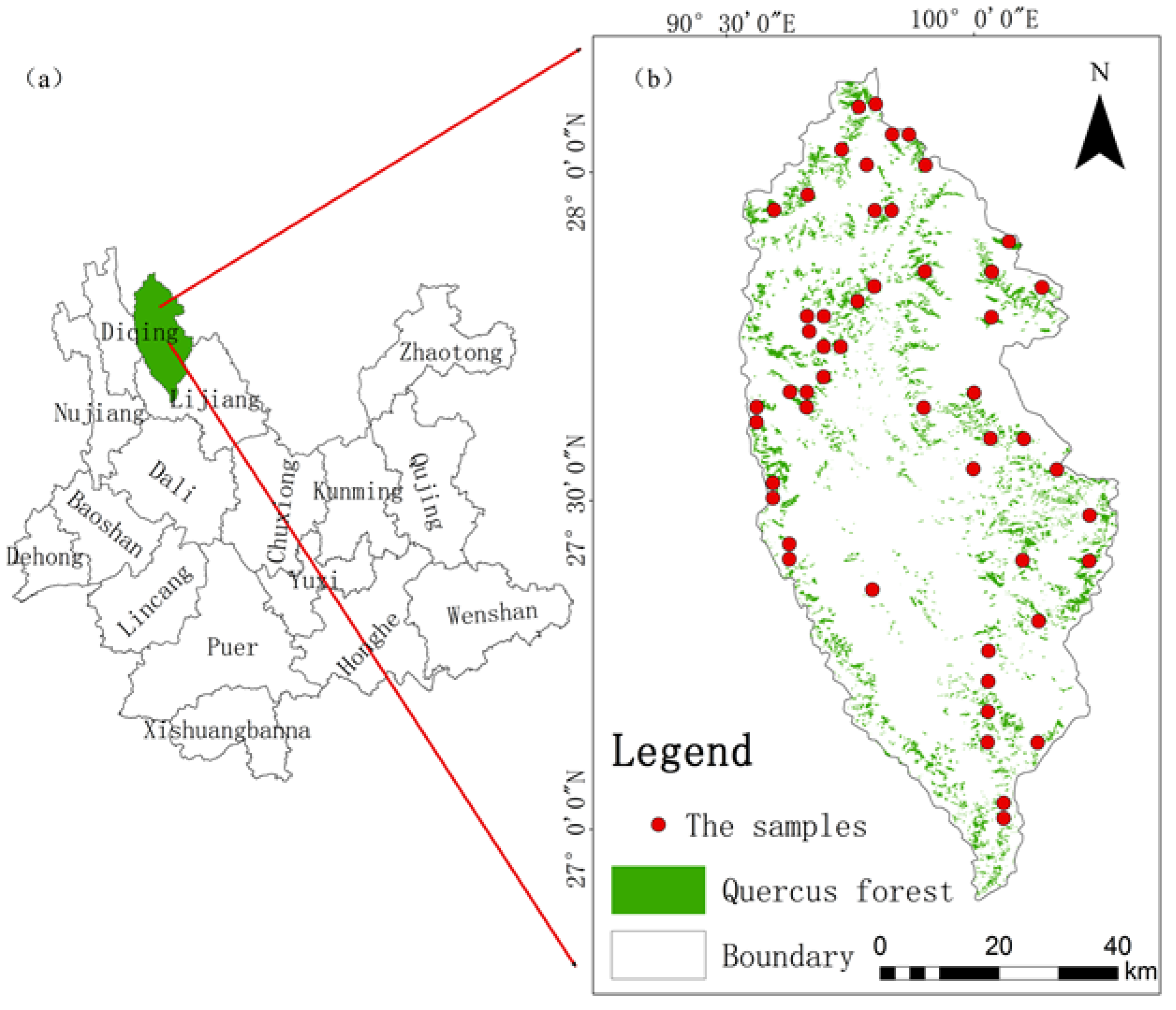
2.1. Study Area

The study was carried out in Shangri-La City, Yunnan Province, China (latitude 26°52′~28°52′ N, longitude 99°20′~100°19′ E), as displayed in Figure 1. It is located in the cold temperate mountain monsoon climate zone; the summer is hot and rainy, whereas winter is cold and dry. Elevation has a substantial altitude interval range, with a median of 3459 m. The annual mean temperature in Shangri-La is 5.5 °C, and annual precipitation is 618.4 mm. Shangri-La City is located in the transition zone from the subtropical evergreen broad-leaved forest vegetation area in Yunnan to the Qinghai–Tibet Plateau vegetation area, and its vegetation distribution is substantially distinct from the north to the south. The site is predominated by Pinus densata, Quercus semicarpifolia, Picea asperata, Pinus yunnanensis and Abies fabri [25].

2.2. Forest Resource Inventory Data

The forest resource inventory data encompasses five dominant tree species: Pinus densata, Quercus aquifolioides, Picea asperata, Pinus yunnanensis and Abies fabri. In total, 52 sample plots with the dominant species of Quercus in the research area were used in this study. They were circular sample plots with a size of 1 hectare, which were generally known as angle gauge controlling sample plots (AGCSP). Within each plot, the average diameter at breast height (DBH) and tree height (H) were recorded. The calculation of the biomass of each plot has two steps. Firstly, the individual-average-standard tree biomass in AGCSP was calculated using the average tree height and average diameter at the breast height of the plot. The individual tree aboveground and underground biomass model of Quercus is shown in Equations (1) and (2). Secondly, the sample plot’s biomass was obtained by combining the single-average-standard tree biomass and the number of Quercus trees. Within 52 sample plots, the minimum, maximum, mean, and standard deviations of the aboveground biomass of different tree species are recorded in

Table 1. Summary information of ground survey sample sites.

Forest Parameters	Value Range	Average Value	Standard Deviation
Aboveground biomass/(t/hm2)	(11.17~274.97)	89.42	58.00
Belowground biomass/(t/hm2)	(2.93~47.45)	22.19	10.44
Total biomass/(t/hm2)	(14.14~215.79)	111.61	67.45

. The maximum is 215.79 t/hm², and the minimum is 14.14 t/hm². The Quercus biomass model we selected in Shangri-La is shown below [26]:

$$M_A={0.07806D}^{2.06321}{H}^{0.57393}$$

(1)

$$M_B={0.055616D}^{2.32664}{H}^{-0.18971}$$

(2)

where M_A is the aboveground biomass (kg/m²), M_B is below-ground biomass (kg/m²), D is the diameter at breast height (cm), and H is the standing height (m).

2.3. Data Acquisition and Processing of GEDI

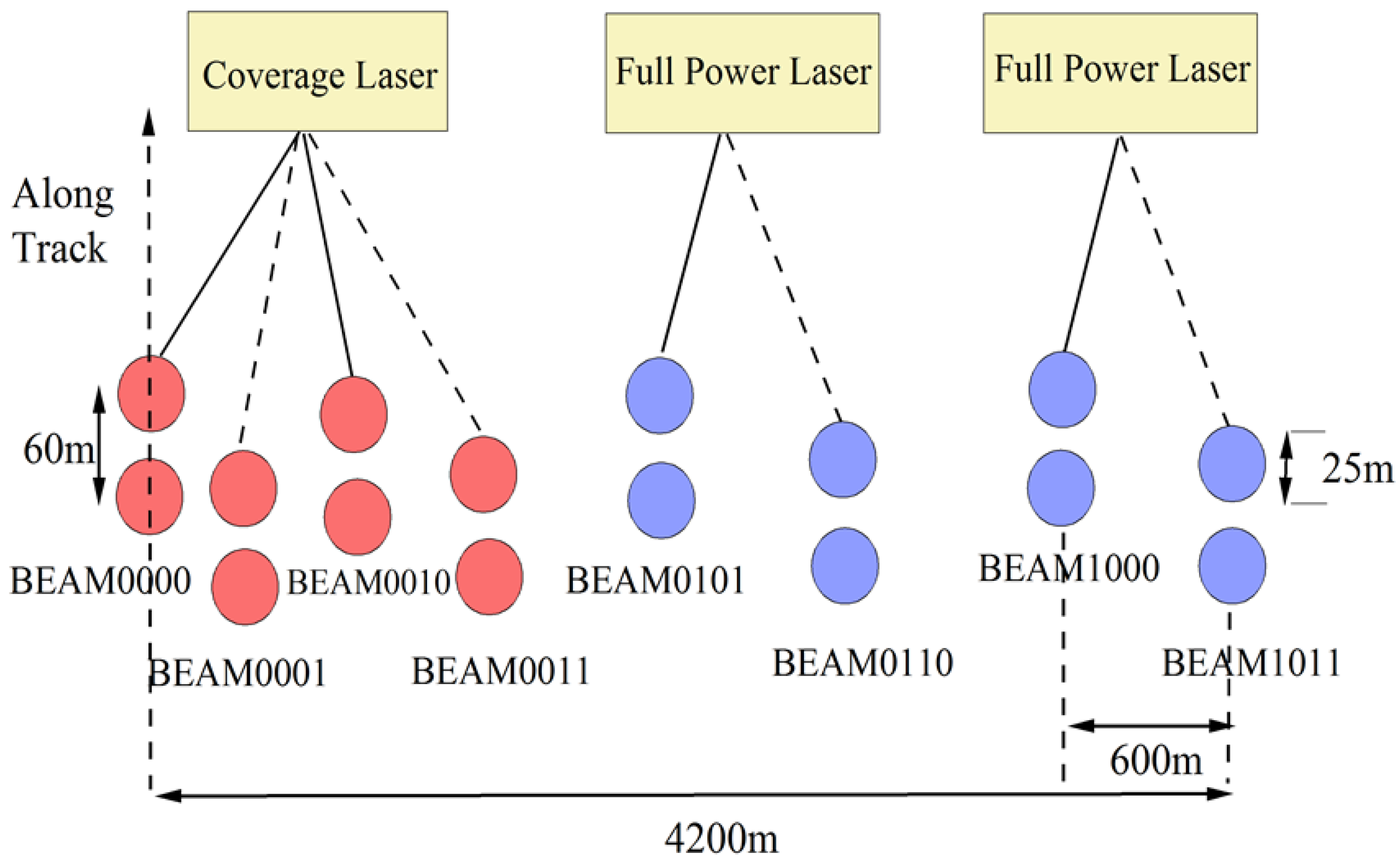
2.3.1. GEDI

GEDI is set to launch from the International Space Station (ISS) in the United States on 5 December 2018, which collects data globally between 51.6° north and south latitudes. The GEDI instrument consists of three lasers, one of which is divided into two beams of weaker energy, producing eight beam ground tracks with approximately 25 m footprint spots and 60 m spacing between large footprints along the tracks, as shown in Figure 2. It contains four product levels of data: L1 is the geolocated return energy waveform data, L2 is the geolocated surface elevation and canopy height products, L3 is the gridded vegetation structure, and L4 is the footprint level and gridded level aboveground biomass products [27].

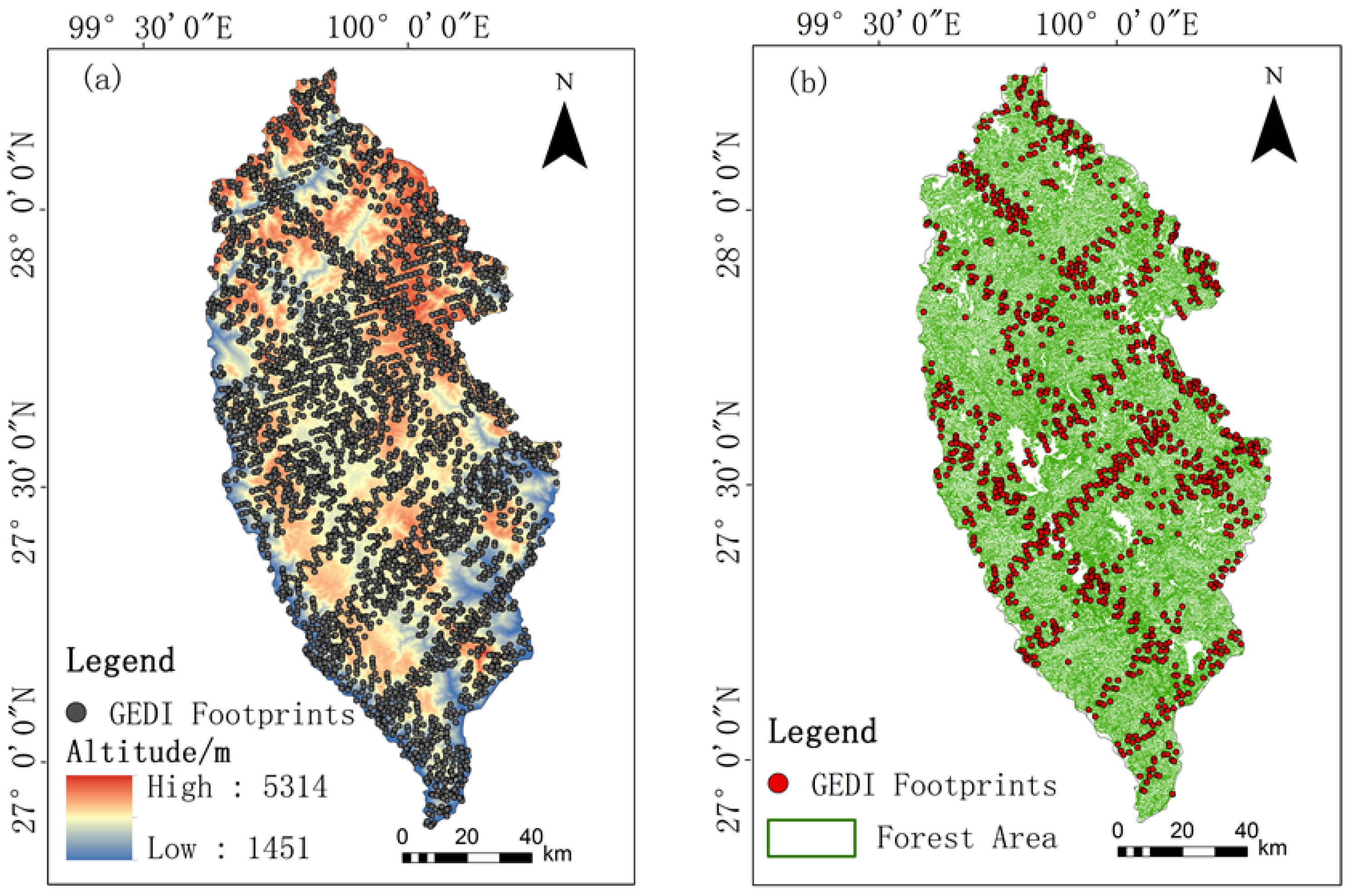
2.3.2. GEDI Data Processing

The data used in our study were GEDI L2B data, compared against the GEDI L2A data. L2B contains biophysical information derived from the geolocated GEDI return waveforms such as total and vertical profiles of canopy cover and plant area index (PAI), the vertical plant area volume density profile (PAVD), and foliage height diversity (FHD). Data at all levels can be downloaded for free through Earthdata Search (https://www.earthdata.nasa.gov, accessed on 6 November 2022). In this study, all GEDI beams in the research area were selected according to the Shangri-La boundary, and a total of 38 data from 23 April 2019 to 4 December 2019 were obtained. By cropping the light spots in the study area, we obtained a total of 3864 spots distributed in Shangri-La. To obtain high-quality GEDI spots, invalid spots were filtered out through the parameters that come with GEDI L2B data and the experience of previous studies [28,29]. The filtering conditions used in this study are as follows:

• Lat_lowestmode, lon_lowestmode: Latitude and longitude can be used to find the spots’ location.
• Sensitivity: Sensitivity is greater than or equal to 0.9 indicates that the spot quality is good; thus, spots with a value less than 0.9 are deleted.
• quality_flag: A quality_flag value of 1 indicates that the laser shot meets criteria based on energy, sensitivity, amplitude, real-time surface tracking quality and difference to a DEM.
• degrade_flag: When this value is 1, it means that the state of the pointing or geolo-cated information is degraded; thus only the spots with degrade_flag = 0 is retained.

After screening the incorrect spots using the four methods mentioned above, we obtained 1307 effective spots in the study area, 880 spots distributed in the forest area, and 427 spots distributed in the non-forest area, as shown in Figure 3. GEDI spots in the study area were selected using the range of latitude and longitude. The parameters information extracted from GEDI L2B are shown in

Table 2. Parameters extracted from GEDI data.

Parameters	Description	Parameters	Description
cover	Total cover, defined as the percentage of the ground covered by the vertical projection of canopy material	modis_nonvegetated	Percentage non-vegetated from MODIS data
pgap_theta	Estimated Pgap(theta) for the selected L2A algorithm	modis_treecover	Percentage of tree cover from MODIS data
pai	Total Plant Area Index	dem_	DEM from GED
leaf_on_doy	Leaf on day of year	leaf_off_doy	Leaf off day of year
pgap_theta_error	Total Pgap(theta) error	rv_aN	integral of the vegetation component in the RX waveform
rg_aN	Integral of the ground component in the RX waveform	sensitivity	Maximum canopy cover that can be penetrated considering the SNR of the waveform
rx_energy_aN	Received waveform energy between toploc and botloc with noise removed	rh100	Height above ground of the received waveform signal start
fhd_normal	Foliage height diversity index calculated by vertical foliage profile normalized by total plant area index.	Lat_lowestmode Lon_lowestmode	latitude and longitude
quality_flag	quality flag	degrade_flag	Degrade flag

_aN (N = 1~6), which means 6 algorithms for GEDI.

.

3. Methods

The primary steps for constructing biomass models based on GEDI data and performing regional-scale extrapolation of footprints biomass are as follows: selection of the interpolation model; evaluation of interpolation accuracy; feature importance ranking; and biomass estimation model construction and assessment (as shown in Figure 4).

3.1. Geostatistical Methods

This study first processed spot data, and then fitted the semi-variance function to determine the model selected for interpolation. Kriging interpolation was performed to obtain light spot polygon information in ArcGIS.

3.1.1. Variance Function

The variance function is a specific tool in geostatistics, which can describe both the structural changes in regionalized variables and their random changes. The variation function can reflect the spatial variation characteristics of regionalized variables, particularly the structure of regionalized variables through randomness; thus, it is also named the variation function and the structure function. Half of it is called the semi-variogram. If the regionalized variable footprint biomass Z(x) satisfies the second-order smooth intrinsic hypothesis, the formula is as follows:

$$\gamma \left(h\right)=\frac{1}{2N\left(h\right)}\sum _{i=1}^{N\left(h\right)}{\left[Z\left(x_i\right)-Z\left(x_i+h\right)\right]}^2$$

(3)

where $\gamma \left(h\right)$ is the biomass variation function; N(h) is the number of pairs of points with a distance equal to h in a certain direction; Z(x_𝑖) is the measured value of biomass of the variable at point x_𝑖; and Z(x_𝑖 + h) is the value of the biomass of the variable at point x_𝑖 deviated from h.

3.1.2. Kriging Interpolation

The Kriging method, also known as spatial local estimation or the spatial local interpolation method, is based on the theory of variogram and structural analysis. It is a method used for linear unbiased optimal estimation of the value of regionalized variables in a restricted area. The formula is as follows:

$$Z_v^{*}\left(x_0\right)={\sum }_{i=1}^n{\lambda }_{i}Z(x_i)$$

(4)

where $Z_v^{*}\left(x_0\right)$ is the estimated biomass at the point to be estimated, $Z\left(x_i\right)$ is the observed biomass at the point to be estimated,${\lambda }_i$ is the weight of each parameter known value, and n is the number of light spots.

3.1.3. Evaluation of Interpolation Accuracy

This research used GS+ software to obtain an optimal variogram model and performed cross-validation to evaluate the accuracy of the Kriging interpolation [30]. The evaluation standard for the fitting effect of the variogram is to first consider the determination coefficient (R²) and the residual size, followed by the range and the nugget value. If the model R² is larger, the residual error is larger, the range is large, and the nugget value is smaller, the best model prediction is indicated [31]. Additionally, is always evaluated using mean error (ME), standard mean error (MSE), mean standard error (ASE), root-mean-square error (RMSE), and standardized root-mean-square error (RMSSE). The formula is as follows:

$$ME=\frac{{\sum }_{i-1}^n\left[\widehat{Z}\left(x_i\right)-Z(x_i)\right]}{n}$$

(5)

$$MSE=\frac{{\sum }_{i-1}^n\left[\widehat{Z}\left(x_i\right)-Z\left(x_i\right)\right]∕\widehat{\sigma }(x_i)}{n}$$

(6)

$$ASE=\sqrt{\frac{{\sum }_{i=1}^n\widehat{\sigma }\left(x_i\right)}{n}}$$

(7)

$$RMSE=\sqrt{\frac{{\sum }_{i=1}^n{\left[\widehat{Z}\left(x_i\right)-Z(x_i)\right]}^2}{n}}$$

(8)

$$RMSSE=\sqrt{\frac{{\sum }_{i=1}^n{\left\{\left[\widehat{Z}\left(x_i\right)-Z\left(x_i\right)\right]∕\widehat{\sigma }(x_i)\right\}}^2}{n}}$$

(9)

where $\widehat{Z}\left(x_i\right)$ is the predicted value of the i at position x, $Z\left(x_i\right)$ is the observed value of the i at position x, and n is the number of light spots.

The 1307 light spots were randomly divided into two parts using the ArcGIS software. In total, 70% of the light spots were used for interpolation, and the remaining 30% were used to verify the final interpolation results. Through the interpolation of light spot data using the geostatistical module, the estimation of each piece of parameter data from point to surface in the whole study area is realized. Combined with the results of cross-validation, SPSS was used to compare the measured and predicted values of the remaining 30 % of the light spots to verify the feasibility of interpolation.

3.2. Biomass Estimation Models

This study combined 3 models to forecast Quercus biomass in Shangri-La: multiple linear regression, support vector regression, and random forest. All of them were implemented using the programming languages in the Rstudio.

3.2.1. Multiple Linear Regressions

The multivariate linear regression model describes a situation in which a dependent variable is affected by multiple independent variables and can quantitatively describe the correlation between variables [32]. The linear regression model of random variable y and general variables x₁, x₂, x₃ … x_p is:

$$y={\beta }_0+{\beta }_1{x}_1+{\beta }_2{x}_2+\cdots +{\beta }_p{\beta }_p+\epsilon$$

(10)

where $y$ is the dependent variable, $x$ is the independent variable, $\epsilon$ is the random error, ${\beta }_0$ is the regression constants, and ${\beta }_1,{\beta }_2,\cdots {\beta }_p$ is the regression coefficient.

3.2.2. Support Vector Regression

A support vector machine is a supervised learning model associated with learning algorithms for data classification and regression analysis [33]. It contains two primary ideas: one is constructing an optimal hyperplane to divide samples in feature space, and the other is mapping samples into a high-dimensional space by applying the nonlinear kernel function, so that it can construct separable problems [34]. The support vector regression algorithm (SVR) is obtained by expanding SVM from a classification problem to a regression problem. The construction of the SVM model is realized by using the SVM function of the e1071 package in Rstudio software. In this study, a radial basis is selected as a kernel function, whereas the penalty coefficient (C) and the mapping parameter (g) are tuned using the tune.SVM function. The values after tuning are set at 1 and 0.5, respectively.

3.2.3. Random Forest

A random forest is a forest composed of numerous randomly generated trees. Each tree is random; thus, they are independent of each other and have no correlation or dependence [35]. Random forest is an enhanced classifier (regressor) constructed of multiple decision trees; when new data enters the random forest, all decision trees will generate classification or prediction results, and the random forest will take the mode or average of these results as the output of the data [36]. Because the random forest selects the sample, each learning decision tree uses a different training set; thus, they can avoid over fitting to some degree.

In the process of constructing decision trees, the importance ranking of variables is needed. Random forest for feature selection usually has two methods. The first method is based on OOB (out of bag) data, also known as out of bag. It is aimed at a decision tree that calculated the fitted result of the corresponding features of OOB data which was brought into the decision tree before and after being disrupted. The second method measures the importance of features by calculating the reduction in the impurity of variables. Because a random forest is composed of trees, the reduction in the decision tree’s impurity before and after the variables’ segmentation can be measured by the change in the residual sum of squares [37]. In Rstudio, the randomForest package provides the function to calculate the significance of variables. When setting the importance = TRUE in the randomForest function, the importance of the variables can be viewed in the returned results. The randomForest package provides four indicators for calculating the importance of variables, namely MeanDecreaseAccuracy, MeanDecreaseGini, %IncMSE and IncNodePurity. When aimed at regression problems, feature selection can be performed by calculating %IncMSE, and IncNodePurity. Since the %IncMSE passed OOB data to verify, it has high credibility in feature selection. Therefore, the results of %IncMSE will be chosen for feature selection in this study.

3.2.4. Evaluation of Biomass Model Accuracy

Due to the small number of ground survey plots, in order to reduce the errors induced by splitting training samples and validation samples, this study used 10-fold cross-validation to assure the stability of the model. Moreover, 10-fold cross-validation divided the data into 10 parts; 9 of them were used as training data, and 1 as test data in turn. Each time, it will acquire a corresponding accuracy rate, and the estimation of this algorithm accuracy is the average precision rate in 10 results [38]. The accuracy of each model was evaluated using the average of R² and RMSE. R² represents the degree of correlation between independent variables and dependent variables, and remains consistently between 0 and 1 if the R² is near 1, implying that the predicted value is closer to the observed data. RMSE is the square root of the mean square error, and is used to measure the average deviation between the predicted value and the observed data—the smaller the value, the better the prediction of the model. Each indicator was calculated as follows:

$$R^2=1-\frac{{\sum }_{i=1}^n{\left(y_i-{\widehat{y}}_i\right)}^2}{{\sum }_{i=1}^n{(y_i-\stackrel{-}{y})}^2}$$

(11)

$$RMSE=\sqrt{\frac{{\sum }_{i=1}^n{\left(y_i-{\widehat{y}}_i\right)}^2}{n-1}}$$

(12)

where 𝑦_𝑖 is the true value; ${\widehat{y}}_i$ is the estimated value; $\stackrel{-}{y}$ is the mean of true value; and n is the number.

4. Results

4.1. Selection of Variance Function

According to the assessment and interpolation method of variance function, the Gaussian, Spherical, linear, and Exponential models were applied to fit the variogram, and the structure of the variogram was performed, from which the optimal model was selected. The structure ratio (C/C₀ + C) indicates the degree of spatial correlation of the system variables, if the structure ratio < 25%, the system has weak spatial correlation; if the structure ratio lies between 25% and 75%, the system has moderate strength spatial correlation; if the resulting ratio > 75%, the system has strong spatial correlation [39]. As shown in

Table 3. Relevant parameter values for each parameter variation function.

Parameter Name	Model	R2	Residual SS	Nugget	Sill	Structural Ratio	Range
sensitivity	Gaussian	0.65	3.14 × 10−5	0	0.05	0.83	0.05
	Spherical	0.65	3.14 × 10−5	0	0.05	0.95	0.06
	Linear	0.13	7.78 × 10−5	0.05	0.06	0.05	0.93
	Exponential	0.68	2.90 × 10−5	0.01	0.05	0.89	0.07
rv	Gaussian	0.52	5553	155.00	907.90	0.83	0.05
	Spherical	0.52	5524	50.00	907.70	0.95	0.05
	Linear	0.04	11076	892.75	911.77	0.02	0.93
	Exponential	0.54	5364	103.00	908.10	0.89	0.05
modis_ nonvegetated	Gaussian	0.26	0.26	0.12	1.28	0.91	0.06
	Spherical	0.26	0.26	0	1.28	0.10	0.07
	Linear	0.82	0.06	1.02	1.48	0.31	0.93
	Exponential	0.80	0.07	1.00	2.04	0.51	4.91
modis_ treecover	Gaussian	0.60	1.23	0.74	5.24	0.86	0.06
	Spherical	0.60	1.23	0.18	5.24	0.97	0.07
	Linear	0.41	1.82	4.66	5.61	0.17	0.93
	Exponential	0.72	0.88	0.61	5.28	0.88	0.11

, except the spherical model of modis_nonvegetated, the structure ratios of rv, modis_treecover, and sensitivity linear models are <25%. Additionally, the proportion of the linear model and exponential model of modis_nonvegetated is between 25% and 75%. The proportion of the remaining models for the other parameters is >80%, indicating that each parameter has a significant spatial correlation when interpolated.

The optimal variance function model was selected using the GS+ software, based on the principle of smaller residuals and larger coefficients of determination. By comparison, the percentage of modis_nonvegetated was fitted slightly better in the linear model than other models; thus, the linear model was selected as the theoretical variance function model. Rv, sensitivity, and modis_treecover have the largest R² and the smallest RSS when using the exponential model, and the exponential model was selected as the optimal variance function model for the Kriging method.

4.2. Validation of Interpolation Results

The mean error (ME), standard mean error (MSE) mean standard error (ASE), root-mean-square error (RMSE), and standardized root-mean-square error (RMSSE) were chosen to evaluate the effect of Kriging interpolation. The standards for evaluation are that the closer the ME and MSE are to 0, the more unbiased the predicted value is. The ASE should be close to the RMSE, and the closer the value is, the higher the validity of the fitted model is. If the ASE is greater than the RMSE, the prediction uncertainty is overestimated; on the contrary, the prediction uncertainty is underestimated. Lastly, the RMSSE should be near 1. The closer the value is to 1, the higher the accuracy of the prediction results [40]. As shown in

Table 4. Cross validation results of Kriging interpolation.

Parameter Name	ME	RMSE	MSE	RMSSE	ASE	R2	Model
sensitivity	0.00	0.02	0.00	1.01	0.02	0.62	Gaussian
rv	10.18	3950.54	0.00	0.90	4378.33	0.71	Spherical
modis_nonvegetated	0.12	9.29	0.01	1.00	9.17	0.81	Linear
modis_treecover	0.00	0.30	0.00	0.98	0.31	0.62	Exponential

, the results of cross-validation showed that the standardized mean of each parameter is near 0, besides the Mean error of rv is 10.18, The rest of the standard root mean squares are close to 1. Additionally, the value of the root mean square is close to the mean standard error. Statistical analysis of the observed and predicted values of the randomly reserved 30% light spots data by SPSS. The outcome demonstrated that the highest accuracy R² of modis_nonvegetated was 0.81, succeeded by 0.71 for the rv and 0.62 both for the sensitivity and modis_treecover. The results also reflected that the Kriging results have great precision and nice spatial prediction for each parameter, and also revealed that using the Kriging method to interpolate the spot property information to the polygon surface is a viable method.

4.3. Variable Correlation Coefficient Matrix and Importance Analysis

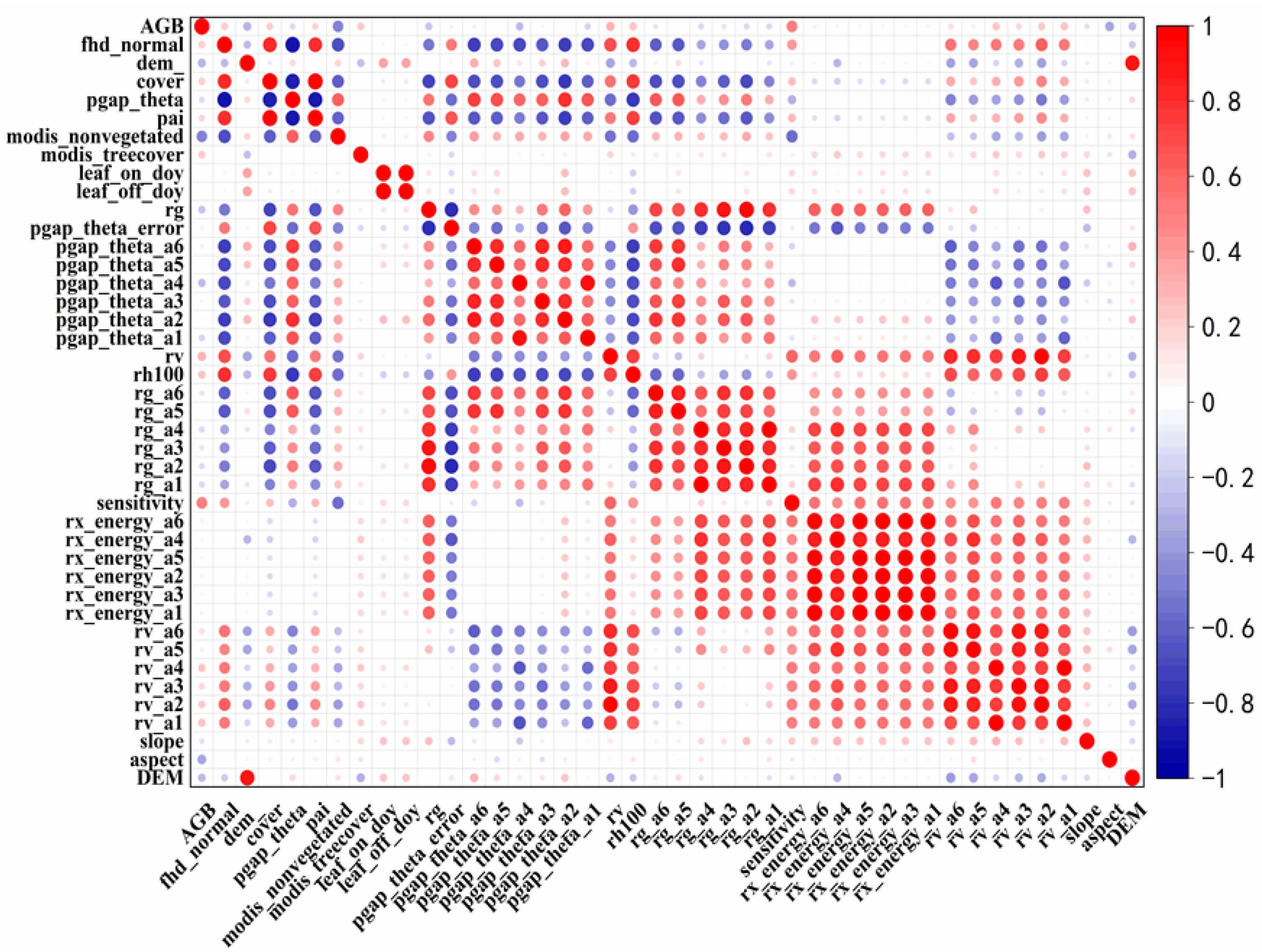
4.3.1. Correlation Analysis of Model Variables

This study selected a total of 41 variable parameters, including 38 parameters extracted from GEDI and 3 topographic factors (aspect, slope, elevation). The parameters from GEDI L2B included cover, fhd_normal, pai, pgap_thea, digital_elevation_model, rg, rh100, rv, sensitivity, rx_enerage, etc. The GEDI parameters with substantial correlation were screened as independent variables of the Biomass estimation model. SPSS 21.0 software was used to analyze the correlation between Quercus biomass and 41 variable parameters of the sample sites by Pearson correlation coefficient analysis, as well as to visualize the correlation coefficient matrix. Two variables that were correlated with biomass at the 0.05 level were aspect and modis_nonvegation; both were significantly negatively correlated with Quercus biomass. One variable correlated with biomass at the 0.01 level was sensitivity, which showed a significant positive correlation. It is indicated that those variables contain information affecting vegetation biomass. The other parameters such as rv, rh100, fhd_normal and, dem from GEDI were related to topography and vegetation also have a certain correlation with Quercus biomass, but the correlation is weak. The correlation analysis is shown in Figure 5.

4.3.2. Selection Results of Characteristic Variables

We used stepwise regression methods and random forest to select the result of feature variables in

Table 5. Results of variable filtering.

Variable Filtering Method	Variable Name
Stepwise regression	Sensitivity, aspect, dem_, slope, rg_a1
Random forest	Sensitivity, aspect, modis_nonvegetated, rv, modis_treecover

. The multiple linear regression models were filtered via the stepwise method, whereas the characteristic variables of the random forest model were graded from the highest to the lowest value of %IncMSE. In Table 5, it can be seen that variables screened using both methods include sensitivity and aspect, which demonstrates that these two variables have a significant influence on Quercus biomass estimation, followed by modis_treecover, rv, and sensitivity; these variables are associated with the forest canopy, suggesting a significant association between biomass and canopy cover. Besides canopy cover, both methods selected aspect, slope, and dem as topographic factors, which implied that the distribution and quantity of Quercus biomass in Shangri-La are impacted by topographic conditions to some extent.

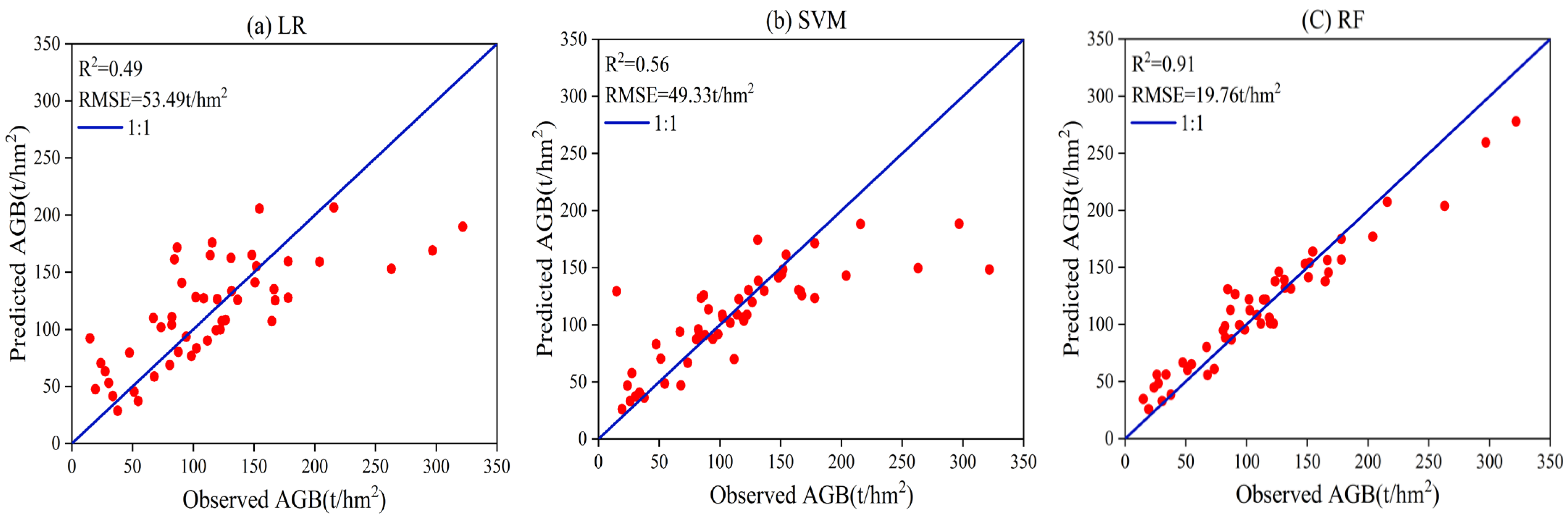
4.4. Accuracy Evaluation of Each Biomass Estimation Models

We used GEDI as the data source, combined with the data from Quercus sample plots of the forest management inventory in Shangri-La. Stepwise regression and random forest were used to optimize the variables extracted from GEDI. The characteristic variables selected in Table 4 were substituted into the multiple linear regressions and random forest algorithm model, respectively, whereas the five characteristic variables selected using random forest were used as the independent variables of support vector regression, and three remote sensing estimation models of Quercus biomass in Shangri-La were established in Figure 6. Contrasting R² and RMSE with each model, the results showed that random forest had the highest estimation accuracy. The five characteristic variables selected using random forest were highly sensitive to the biomass of alpine mountain Quercus and could better simulate its biomass. Compared with the three biomass estimation models we have constructed, it can be seen that the random forest model (R² = 0.91, RMSE = 19.76 t/hm²) is superior to the support vector regression model (R² = 0.56, RMSE = 49.33 t/hm²) and multiple linear regression model (R² = 0.49, RMSE = 53.49 t/hm²) in terms of fitting degree and error.

4.5. Spatial Distribution Analysis of Total Biomass

Figure 7 demonstrated the spatial distribution of biomass induced by cooperative Kriging in Shangri-La. According to the calculation, the average total biomass of 52 plots in Shangri-La was 111.61 t/hm². The average aboveground and underground biomass of the whole Shangri-La Quercus predicted by the model was 114.33 t/hm². The total biomass was about 1.26 × 10⁷ t/hm², it was distributed between 26.48 and 257.63 t/hm². The result was very close to the observed data from the forest management inventory in 2016. The distribution altitude of Quercus in Shangri-La is mainly in 1451 and 5314 m, which fits the characteristics that Quercus distributed in 2000 and 4500 m of southwest China in sunny slopes, valley Quercus forest, or pine–Quercus forest. As shown in Figure 7, the distribution of Quercus was extremely dispersed and did not have obvious regulation. The areas with high biomass were distributed at altitudes of 3000 and 4000 m in the west and northeast, mainly in Wujin Township, Geza Township, and Luoji Township. Additionally, the areas with low biomass were distributed in the north of Dongwang Township, the south of Jinjiang Town and Tiger Leap Gorge Town, and the northeast of NiXi Township. There are many crest lines distributed in the north–south direction of Shangri-La, and Quercus are primarily distributed in the sunny slope; thus, the crest lines played a certain influence on the sunlight of Quercus. Therefore, it can be seen that the biomass content of Quercus is low in the north of Dongwang Township and the south of Jinjiang Town.

5. Discussion

The three-dimensional structure of forests is an important basis for estimating changes in forest biomass due to human activities or natural disturbances, as well as a crucial component for evaluating forest habitat quality and biodiversity on a regional scale [41]. Investigators need to develop large-scale, region-wide forest biomass estimation models by remote sensing and costly surveys. Therefore, NASA’s GEDI mission brings a broader perspective on forest biomass estimation. Our study solved the problem of incomplete coverage of GEDI spaceborne lidar spots by using Kriging interpolation. This method has great potential in estimating forest biomass on a county scale and also demonstrated the feasibility of implementation on a larger scope.

5.1. Precision Analysis of Estimation Results

The data of the Quercus small class in the forest resources inventory in 2016 were used as ground-measured data. Through calculation and prior studies, the growth rate of the Shangri-La Quercus volume was 4.04%. The total volume of Quercus in Shangri-La in 2019 was obtained by multiplying the growth rate by the measured volume in 2016. Finally, the total biomass of Quercus in 2019 was calculated to be 1.22 × 10⁷ t/hm² by using the volume–biomass conversion model. Compared with the observed data, our results (the average biomass was 114.33 t/hm², and the total biomass was 1.26 × 10⁷ t/hm²) that used GEDI spaceborne lidar to predict the Quercus biomass by Kriging interpolation are in the same order of magnitude. In previous studies that estimated biomass using remote sensing technology, Wang et al. [42] combined topography, vegetation, and soil factors, using an analytic hierarchy process (AHP) to assign weights to different indicators and determine weight factors. Using the remote sensing information model, the total biomass of Quercus in Shangri-La was estimated to be 1.40 × 10⁷ t/hm² and the average biomass was 112.99 t/hm². Xie et al. [43], based on 277 field survey plots and Landsat 8/OLI images, on the basis of the K-nearest neighbor (k-NN) model optimized by the genetic algorithm in the early stages, optimized the three parameters of K-NN on the pixel scale, estimated the aboveground biomass of four typical forest types in the study area using remote sensing and spatial inversion, and found that the AGB of Quercus was 1.3 × 10⁷ Mg. Compared with the observed values of the forest resources inventory data, there were some errors in the estimation of Quercus biomass based on traditional optical remote sensing. Their results overestimated Quercus biomass, which proved the influence of traditional optimal remote sensing saturation on forest biomass estimation results. However, researchers found that this influence can be weakened by using different remote sensing feature factors related to vegetation [8]. Guo et al. [44] extracted the red, red-edge, and near-infrared bands from Sentinel-2 images to construct vegetation indices such as TVI, CARI, IRECI, and TSAVI. These vegetation indices can respond quickly to small changes in the chlorophyll content and canopy structure of grassland vegetation, thus improving the accuracy of grassland biomass estimation, while being able to weaken the effect of saturation in the red-edge region at larger AGB values. In order to weaken the effect of light saturation phenomenon on accuracy, the extraction of backscatter coefficients and texture features from SAR can be considered in future research to invert the biomass together with information such as canopy height and vertical structure provided by GEDI.

5.2. Analysis of the Interpolation Result

Spatial interpolation uses observations at known locations to predict values at unknown locations; this has the potential to take full advantage of dense spaceborne lidar observations in mapping large-scale forest canopy height. Spaceborne lidar footprints are generally evenly distributed along ground tracks instead of being randomly distributed. As a result, forest biomass interpolated from a single spaceborne lidar platform may display a strong strip effect across ground tracks [45]. In order to avoid this problem and to obtain high-quality data, before using GEDI data for interpolation, some spots with bad quality on the strip were filtered; therefore, some adjacent strips and neighboring spots on the same strip will be deleted to reduce the strip effect in the later interpolation. Because the scanning track of ICESat-2 is different from GEDI, researchers can fuse different pieces of spaceborne lidar data in the future. For example, this could be carried out using ICESat-2 to disrupt the uniform distribution of light spots, so as to weaken the band effect during interpolation and obtain high-precision biomass estimation results.

The geostatistics-based method of spot parameter interpolation has certain requirements on the number and distribution of spots. Only by fitting the variation law of parameters in the whole region can the estimation accuracy be guaranteed. The main limiting factors that affected the estimation accuracy of geostatistics include the accuracy of spot parameters, the interpolation method, and the selection of the interpolation model [46]. Liu et al. [45] developed a natural-network-guided interpolation (NNGI) method based on an interpolation framework to map wall-to-wall forest canopy height distribution by fusing GEDI and ICESat-2 ATLAS data. Comparison with the validation data indicated that NNGI successfully derived forest canopy height distribution of China at 30 m resolution. The R² and RMSE of the NNGI interpolated forest canopy height ranged from 0.55 to 0.60 and from 4.88 m to 5.32 m when compared with GEDI validation footprints, drone-lidar validation data, and field measurements. In this paper, the optimal model for interpolation of each GEDI parameter is determined by calculating the semi-variance function by GS+ software. Compared with the default model for interpolation, the interpolation results obtained from the optimal model selected by calculating the semi-variance function had higher levels of accuracy. The best result was achieved by interpolating modis _ nonvegetated using a linear model, and its R² was 0.81. Combining our results and those of Liu demonstrated the feasibility of using interpolation to extend the spot data to the whole region.

5.3. The Influence of Sample Size on Model Accuracy

Many uncertain problems exist in data acquisition, the selection of characteristic factors, model parameter selection, and modeling methods when estimating biomass [47]. Among the factors mentioned above, model uncertainty is a major problem to be solved. The number of samples used for remote sensing modeling has a significant effect on the uncertainty caused by model parameters, and the uncertainty gradually decreases as the number of samples increases [48]. Wu et al. [47] selected 1/4 samples, 1/2 samples, 3/4 samples, and all samples from different biomass interval samples in a recoverable form to compare the effects of different samples on modeling accuracy. SVM, RF, and SGB all showed that the accuracy of biomass estimation gradually increased with the rise in sample size.

In traditional statistical sampling data, 30 for a small sample and 50 for a large sample are only empirical sample sizes; the larger the number of samples, the better the model’s reliability. At the same time, the influence of the number of samples on the accuracy of the model depends on the modeling method. Some models are suitable for large samples, whereas others can obtain better results by using small samples. Fu demonstrated that increasing the sample sizes can enhance the modeling precision, especially for the SVM model. However, the changes in accuracy in PLS and the K-NN algorithm verified that increasing sample sizes cannot necessarily improve accuracy [49]. Therefore, different estimation methods need to find the most suitable sample sizes. In addition to the number of samples, the distribution, size and representativeness of samples are also crucial parameters. José et al. proved that the design size of sample area can improve the prediction accuracy of biomass [50]. When the sample area was increased from 400 km² to 1000 km², the prediction accuracy of AGB is significantly improved; however, there was no obvious change when the sample area increased to 2200 km². In the process of using machine learning methods to inverse biomass, it is crucial to determine the optimal number of samples for different models, which greatly affects the final biomass estimation accuracy. Shu et al. [51] suggested a new optimizing method that combined the theory of variance function in Geostatistics and value coefficient (VC) in value engineering. The random forest regression (RFR), nearest neighbor (K-NN) method and partial least squares regression (PLSR) were conducted to analyze the change in model accuracy under different samples and determine the optimal number of samples for each model. Although some scholars have analyzed the modeling accuracy of different sample sets, the combination of the control method of sample number and the modeling method needs to be further studied. In total, 52 samples were selected in this study, which is in accordance with a big sample standard. To improve the estimation accuracy of biomass, the optimal samples for estimation models can be determined by decreasing or increasing the number of samples subsequently.

5.4. Effect of Model Selection and Optimization on Estimation Accuracy

With the deepening research on nonlinear biomass models recent years, more and more machine learning methods, such as K-order nearest neighbor, random forest, partial least squares, artificial neural network, and support vector machine, have been applied to explore the relationship between remote sensing factors and forest biomass.

This study used correlation analysis to select independent parameters that were closely related to biomass from a large of number remote sensing characteristic factors by constructing a remote sensing estimation model of forest biomass. Three modeling methods, multiple linear stepwise regressions, support vector machine, and random forest, were compared to estimate Quercus biomass, respectively. Through comparison, it was found that multiple linear regressions cannot reflect the distribution of field biomass. The R²; of its basic parametric model was generally low, and the results were similar to those of other studies [14,52]. In contrast, random forests can effectively describe the complex nonlinear relationships between forest biomass and remotely sensed feature data. Studies have shown that non-parametric models can effectively estimate vegetation parameters. However, for forest ecosystems, the estimation accuracy of general nonparametric models is still limited [35]. Additionally, random forest has strong anti-noise ability and can effectively deal with high-dimensional data, which has superior accuracy and robustness for vegetation parameter estimation such as leaf area index (LAI) and growing stem volume (GSV) [53]. In addition, RF can improve the estimation accuracy by evaluating the importance of variables to form a combination of variables more suitable for AGB estimation [54].

It has been pointed out that parameter selection has an important influence on the modeling algorithm. In this study, two machine learning algorithms are selected, and the parameters corresponding to each algorithm were set with reference to the existing literature based on the observed influence of the parameter adjustment process on modeling accuracy. In Rstudio, the support vector regression is implemented using the svm function in the package ‘e1071′ and selected radial as the kernel function, whereas the penalty coefficient (c) and the mapping parameter (g) are optimized using the tune.svm function; the optimized values were set to 1 and 0.5, respectively. There are two important parameters, ntree and mtry—the number of decision trees based on the number of samples and number of random features—in the randomForest package. In this study, through the training of the model, ntree was set to 400, and mtry was set as the default value. The model R² after tuning was higher than the result using the default value. However, the applicability of the estimated model parameters was inconsistent for different forest types and the spatial distribution of the biomass [55]. Therefore, it is necessary to develop variable selection methods that can meet the demand for AGB estimation under different forest cover conditions. To further improve the accuracy of AGB estimation and reduce the error transfer in the modeling process, we can select other machine learning methods that are suitable for processing multidimensional data, such as using K-nearest neighbors (KNN) [43] or deep learning [56] for further testing. In addition, we can try to use the L-M algorithm [57] for random forest hyper parameter tuning, which can reduce the number of iterations in the optimization process and make full use of the information from each test point [58].

6. Conclusions

Our study showed that by using the variance function in geostatistics for biomass estimation, selecting optimal interpolation models to obtain polygon information, and then building estimation models using the observed data of Quercus biomass in Shangri-La, we can obtain the forest biomass at a county-wide scale. Meanwhile, the results also showed that interpolating spot data to a polygon of GEDI L2B data by Kriging can solve the scale move problem, and realize the biomass information on extended from ‘point’ to ‘polygon’. This method may provide a new opportunity for solving the issue that spaceborne lidar cannot supply wall-to-wall biomass data and may provide a new research direction for effectively estimating forest biomass using GEDI.

Although this study demonstrated the feasibility of GEDI L2B data for estimating biomass, it still needs additional research in the future for the continuous distribution of GEDI data to affect the interpolation accuracy. The next steps can be considered to combine GEDI with ICESat-2 using different interpolation methods to improve the prediction accuracy of the forest biomass. Meanwhile, joint inversion with other remote sensing data such as Landsat and Sentinel can also be attempted in order to acquire a wall-to-wall and high-precision biomass distribution map.

References

1. FAO. The State of the World’s Forests 2018: Forest Pathways to Sustainable Development; United Nations: New York, NY, USA, 2018. [Google Scholar] [CrossRef]
2. Sandra, B. Measuring Carbon in Forests: Current Status and Future Challenges. Environ. Pollut. 2002, 116, 363–372. [Google Scholar] [CrossRef]
3. Brown, S.; Gillespie, A.J.; Lugo, A.E. Biomass Estimation Methods for Tropical Forests with Applications to Forest Inventory Data. Forest Sci. 1989, 4, 881–902. [Google Scholar]
4. Tuominen, S.; Eerikainen, K.; Schibalski, A.; Haakana, M.; Lehtonen, A. Mapping Biomass Variables with a Multi-Source Forest Inventory Technique. Silva Fenn. 2010, 44, 109–119. [Google Scholar] [CrossRef]
5. Potapov, P.; Li, X.; Hernandez-Serna, A.; Tyukavina, A.; Hansen, M.C.; Kommareddy, A.; Pickens, A.; Turubanova, S.; Tang, H.; Silva, C.E. Mapping Global Forest Canopy Height through Integration of GEDI and Landsat Data. Remote Sens. Environ. 2021, 253, 112–165. [Google Scholar] [CrossRef]
6. Liu, X.; Yang, L.; Liu, Q. Review of Forest Aboveground Biomass Inversion Methods Based on Remote Sensing Technology. Ntal. Remote Sens. Bull. 2015, 19, 62–74. (In Chinese) [Google Scholar]
7. Zhao, P.; Liu, D.; Wang, G.; Wu, C.; Huang, Y.; Yu, S. Examining Spectral Reflectance Saturation in Landsat Imagery and Corresponding Solutions to Improve Forest Aboveground Biomass Estimation. Remote Sens. 2016, 8, 469. [Google Scholar] [CrossRef]
8. Arévalo, P.; Baccini, A.; Woodcock, C.E.; Olofsson, P.; Walker, W.S. Continuous Mapping of Aboveground Biomass Using Landsat Time Series. Remote Sens. Environ. 2023, 288, 113–483. [Google Scholar] [CrossRef]
9. Dinesh, B.I.; Frédéric, R.; Pierre, B.; Sylvie, G.; Yves, B.; David, P. Fire Disturbance Data Improves the Accuracy of Remotely Sensed Estimates of Aboveground Biomass for Boreal Forests in Eastern Canada. Remote Sens. Appl. 2017, 8, 71–82. [Google Scholar] [CrossRef]
10. Zhang, J.; Rivard, B.; Sánchez-Azofeifa, A.; Castro-Esau, K. Intra-and Inter-class Spectral Variability of Tropical Tree Species at La Selva, Costa Rica: Implications for Species Identification Using HYDICE Imagery. Remote Sens. Environ. 2006, 105, 129–141. [Google Scholar] [CrossRef]
11. Svein, S.; Rasmus, A.; Terje, G.; Erik, N.; Dan, J.W. Estimating Spruce and Pine Biomass with Interferometric X-band SAR. Remote Sens. Environ. 2010, 114, 2353–2360. [Google Scholar] [CrossRef]
12. Atwood, D.K.; Andersen, H.-E.; Matthiss, B.; Holecz, F. Impact of Topographic Correction on Estimation of Aboveground Boreal Biomass Using Multi-temporal, L-Band Backscatter. IEEE J. Sel. Top. Appl. Earth Obs. Remote Sens. 2014, 7, 3262–3273. [Google Scholar] [CrossRef]
13. Xi, Z.; Xu, H.; Xing, Y.; Gong, W.; Chen, G.; Yang, S. Forest Canopy Height Mapping by Synergizing ICESat-2, Sentinel-1, Sentinel-2 and Topographic Information Based on Machine Learning Methods. Remote Sens. 2022, 14, 364. [Google Scholar] [CrossRef]
14. Jiang, F.; Zhao, F.; Ma, K.; Li, D.; Sun, H. Mapping the Forest Canopy Height in Northern China by Synergizing ICESat-2 with Sentinel-2 Using a Stacking Algorithm. Remote Sens. 2021, 13, 1535. [Google Scholar] [CrossRef]
15. Saarela, S.; Holm, S.; Healey, S.P. Comparing Frameworks for Biomass Prediction for the Global Ecosystem Dynamics Investigation. Remote Sens. Environ. 2022, 278, 113074. [Google Scholar] [CrossRef]
16. Musthafa, M.; Singh, G. Forest Above-ground Woody Biomass Estimation Using Multi-temporal Space-borne LiDAR Data in a Managed Forest at Haldwani, India. Adv. Space Res. 2022, 69, 3245–3257. [Google Scholar] [CrossRef]
17. Xie, D.; Li, G.; Zhao, Y.; Yang, X.; Tang, X.; Fu, A.U.S. GEDI Space-based Laser Altimetry System and Its Applications. Space Int. 2018, 12, 39–44. (In Chinese) [Google Scholar]
18. Adam, M.; Urbazaev, M.; Dubois, C.; Schmullius, C. Accuracy Assessment of GEDI Terrain Elevation and Canopy Height Estimates in European Temperate Forests: Influence of Environmental and Acquisition Parameters. Remote Sens. 2020, 12, 3948. [Google Scholar] [CrossRef]
19. Hakkenberg, C.R.; Tang, H.; Burns, P.; Goetz, S.J. Canopy Structure from Space Using GEDI Lidar. Front. Ecol. Environ. 2023, 21, 55–56. [Google Scholar] [CrossRef]
20. Wang, C.; Elmore, A.J.; Numata, I.; Cochrane, M.A.; Lei, S.G.; Hakkenberg, C.R.; Li, Y.; Zhao, Y.; Tian, Y. A Framework for Improving Wall-to-Wall Canopy Height Mapping by Integrating GEDI LiDAR. Remote Sens. 2022, 14, 3618. [Google Scholar] [CrossRef]
21. Rishmawi, K.; Huang, C.; Zhan, X. Monitoring Key Forest Structure Attributes Across the Conterminous United States by Integrating GEDI LiDAR Measurements and VIIRS Data. Remote Sens. 2021, 13, 442. [Google Scholar] [CrossRef]
22. Laura, D.; Amy, N.; Steven, H.; Nathan, T.; Temilola, F.; Marc, S.; Carlos, A.S.; John, A.; Scott, B.L.; Michelle, H.; et al. Biomass Estimation from Simulated GEDI, ICESat-2 and NISAR Across Environmental Gradients in Sonoma County, California. Remote Sens. Environ. 2020, 242, 111779. [Google Scholar] [CrossRef]
23. Silva, C.A.; Duncanson, L.; Neuenschwander, A.; Thomas, N.; Hofton, M.; Fatoyinbo, L.; Simard, M.; Marshak, C. Fusing Simulated GEDI, ICESat-2 and NISAR Data for Regional Aboveground Biomass Mapping. Remote Sens. Environ. 2021, 253, 112234. [Google Scholar] [CrossRef]
24. Sun, M.; Cui, L.; Park, J.; García, M.; Zhou, Y.; He, L.; Zhang, H.; Zhao, K.G. Evaluation of NASA’s GEDI Lidar Observations for Estimating Biomass in Temperate and Tropical Forests. Forests 2022, 13, 1686. [Google Scholar] [CrossRef]
25. Song, F. Current Status and Characteristics of Forest Resources in Shangri-La County. J. West China For. Sci. 2008, 122, 124–128. (In Chinese) [Google Scholar]
26. State Forestry Administration of China (SFAC). Tree Biomass Models and Related Parameters to Carbon Accounting for Quercus; State Forestry Administration: Beijing, China, 2016. (In Chinese)
27. Chen, L.; Ren, C.; Bao, G.D.; Zhang, B.; Wang, Z.M.; Liu, M.Y.; Man, W.D.; Liu, J.F. Improved Object-Based Estimation of Forest Aboveground Biomass by Integrating LiDAR Data from GEDI and ICESat-2 with Multi-Sensor Images in a Heterogeneous Mountainous Region. Remote Sens. 2022, 14, 2743. [Google Scholar] [CrossRef]
28. Han, M.; Xing, Y.; Li, G.; Huang, J.; Cai, L. Comparison of the Accuracy of the Maximum Canopy Height and Biomass Inversion of the Data of Different GEDI Algorithm. J. Cent. South Univ. For. Technol. 2022, 42, 72–82. (In Chinese) [Google Scholar]
29. Liu, L.; Wang, C.; Nie, S.; Zhu, X.; Xi, X.; Wang, J. Analysis of the Influence of Different Algorithms of GEDI L2A on the Accuracy of Ground Elevation and Forest Canopy Height. J. Univ. Chin. Acad. Sci. 2022, 39, 502–511. (In Chinese) [Google Scholar]
30. Cai, C.; Cao, S.; Kong, F.; Hu, L.; Liu, T.; Sun, W.; Wang, L. A Dataset of Spatial Distribution of Spruce Aboveground Biomass in Western Tianshan Mountains, Xinjiang in 2014. Chin. Sci. Data 2022, 7, 250–263. (In Chinese) [Google Scholar]
31. Ying, C.L.; Ming, Y.L.; Zhen, Z.L.; Chao, L. Combining Kriging Interpolation to Improve the Accuracy of Forest Aboveground Biomass Estimation Using Remote Sensing Data. IEEE Access 2020, 8, 128124–128139. [Google Scholar] [CrossRef]
32. Liao, Y.; Zhang, J.; Bao, R.; Xu, D.; Wang, S.; Han, D. Estimation of Aboveground Biomass Dynamics of Pinus densata by Introducing of Topographic Factors. Chin. J. Ecol. 2022, 1–12. (Online first Publish) (In Chinese) [Google Scholar]
33. Pen, H.; Chen, G.; Chen, X.; Liu, Z.; Yao, C. Hybrid Classification of Coal and Biomass by Laser-induced Breakdown Spectroscopy Combined with K-means and SVM. Plasma Sci. Technol. 2019, 21, 64–72. [Google Scholar] [CrossRef]
34. Raúl, H.; María, T.L.; Juan, D.; Darío, D.; Montealegre Antonio, L.M.; Alberto, M.; Sergio, R. Assessing GEDI-NASA System for Forest Fuels Classification Using Machine Learning Techniques. Int. J. Appl. Earth Obs. 2023, 116, 103175. [Google Scholar] [CrossRef]
35. Qian, C.H.; Qiang, H.Q.; Wang, F.; Li, M.Y. Estimation of Forest Aboveground Biomass in Karst Areas Using Multi-Source Remote Sensing Data and the K-DBN Algorithm. Remote Sens. 2021, 13, 5030. [Google Scholar] [CrossRef]
36. Brown, S.; Narine, L.; Gilbert, J. Using Airborne Lidar, Multispectral Imagery, and Field Inventory Data to Estimate Basal Area, Volume, and Aboveground Biomass in Heterogeneous Mixed Species Forests: A Case Study in Southern Alabama. Remote Sens. 2022, 14, 2708. [Google Scholar] [CrossRef]
37. You, H. R Language Prediction in Practice; Electronic Industry Press: Beijing, China, 2016; pp. 203–204. (In Chinese) [Google Scholar]
38. Liang, Z.; Li, Z.; Lai, C.; Lin, Z.; Li, T.; Zhang, J. Application of 10-fold Cross-validation in the Evaluation Generalization Ability of Prediction Models and Realization in R. Chin. J. Hosp. Stat. 2020, 27, 289–292. (In Chinese) [Google Scholar]
39. Du, H.; Zhou, G.; Fan, W.; Ge, H.; Xu, X.; Shi, Y.; Fan, W. Spatial Heterogeneity and Carbon Contribution of Aboveground Biomass of Moso Bamboo by Using Geostatistical Theory. Plant Ecol. 2010, 207, 131–139. [Google Scholar] [CrossRef]
40. Meng, L. Distribution of Forest Biomass for Main Forest Types in Tahe Forestry Administration of Daxinganling Based on Geostatistics; Northeast Forestry University: Harbin, China, 2017. (In Chinese) [Google Scholar]
41. Ahmad, A.; Gilani, H.; Ahmad, S.R. Forest Aboveground Biomass Estimation and Mapping through High-Resolution Optical Satellite Imagery—A Literature Review. Forests 2021, 12, 914. [Google Scholar] [CrossRef]
42. Wang, J.; Cheng, P.; Xu, S.; Wang, X.; Cheng, F. Forest Biomass Estimation in Shangri-La Based on Remote Sensing. J. Zhejiang AF Univ. 2013, 30, 325–329. (In Chinese) [Google Scholar]
43. Xie, F. Estimation and Mapping of Forest Aboveground Biomass Based on k-NN Model and Remote Sensing; Southwest Forestry University: Kunming, China, 2019. (In Chinese) [Google Scholar]
44. Guo, R.; Fu, S.; Hou, M.; Liu, J.; Miao, C.; Meng, Y.; Feng, Q.; He, J.; Qian, D.; Liang, T. Remote Sensing Retrieval of Natural Grassland Biomass in Menyuan County, Qinghai Province experimental area based on Sentinel-2 data. Acta Pratacult. Sin. 2023, 32, 15. (In Chinese) [Google Scholar]
45. Liu, X.; Su, Y.; Hu, T.; Yang, Q.; Liu, B.; Deng, Y.; Tang, H.; Tang, Z.; Fang, J.; Guo, Q. Neural Network Guided Interpolation for Mapping Canopy Height of China’s Forests by Integrating GEDI and ICESat-2 Data. Remote Sens. Environ. 2022, 269, 112844. [Google Scholar] [CrossRef]
46. Semko, A.; Alireza, S.; Fatemeh, S. The Soil Slope Stability in Failure with the Use of the Random Process Based on the Kriging’s Interpolation Model. J. Civ. Construct. Environ. Eng. 2022, 7, 63–72. [Google Scholar]
47. Wu, C. Regional Biomass Estimation and Application Based on Remote Sensing; Zhejiang University: Hangzhou, China, 2016. (In Chinese) [Google Scholar]
48. Li, H.; Mao, Z.; Shi, H.; Xiao, H. Model Uncertainty in Forest Biomass Estimation. Acta Ecol. Sin. 2017, 37, 7912–7919. [Google Scholar] [CrossRef]
49. Fu, M.; Li, Z.; Qing, T. Optimizing the K-nearest Neighbors Technique for Estimating Pinus Densata Aboveground Biomass Based on Remote Sensing. J. Zhejiang A F Univ. 2019, 36, 515–523. (In Chinese) [Google Scholar]
50. José, L.H.; Juan, M.D.; Kristofer, D.; Richard, B.; Fernando, T.; Alicia, P.; Juan, P.C.; Gonzalo, S.; David, L. Improving Species Diversity and Biomass Estimates of Tropical Dry Forests Using Airborne LiDAR. Remote Sens. 2014, 6, 4741–4763. [Google Scholar] [CrossRef]
51. Shu, Q.; Xi, L.; Wang, K.; Xie, F.; Pang, Y.; Song, H. Optimization of Samples for Remote Sensing Estimation of Forest Aboveground Biomass at the Regional Scale. Remote Sens. 2022, 14, 4187. [Google Scholar] [CrossRef]
52. Jiang, F.; Sun, H.; Li, C.; Ma, K.; Chen, S.; Long, J.; Ren, L. Retrieving the Forest Aboveground Biomass by Combined Red-edge Bands of Sentinel-2 and GF-6. Acta Ecol Sin. 2021, 41, 8222–8236. (In Chinese) [Google Scholar]
53. Jiang, F.; Kutia, M.; Ma, K.; Chen, S.; Long, J.; Sun, H. Estimating the Aboveground Biomass of Coniferous Forest in Northeast China Using Spectral Variables, Land Surface Temperature and Soil Moisture. Sci. Total Environ. 2021, 785, 147335. [Google Scholar] [CrossRef]
54. García-Gutiérrez, J.; Martínez-Álvarez, F.; Troncoso, A.; Riquelme, J.C. A Comparison of Machine Learning Regression Techniques for LiDAR-derived Estimation of Forest Variables. Neurocomputing 2015, 167, 24–31. [Google Scholar] [CrossRef]
55. Lu, D.; Chen, Q.; Wang, G.; Liu, L.; Li, G.; Moran, E. A Survey of Remote Sensing-based Aboveground Biomass Estimation Methods in Forest Ecosystems. Int. J. Digit. Earth 2016, 9, 63–105. [Google Scholar] [CrossRef]
56. Li, C. Evaluation of Garlic Based on Convolutional Neural Network; Shandong Agricultural University: Taian, China, 2022. (In Chinese) [Google Scholar]
57. Seppanen, J.; Antropov, O.; Jagdhuber, T. Improved Characterization of Forest Transmissivity Within the L-MEB Model Using Multisensor SAR Data. IEEE Geosci. Remote Sens. 2017, 14, 1408–1412. [Google Scholar] [CrossRef]
58. Song, H.; Xi, L.; Shu, Q.; Wei, Z.; Qiu, S. Estimate Forest Aboveground Biomass of Mountain by ICESat-2/ATLAS Data Interacting Cokriging. Forests 2023, 14, 13. [Google Scholar] [CrossRef]
Figure 1. (a) is the location of Shangri-La in Yunnan Province; (b) is the distribution of Quercus and sample sites in Shangri-La.
Forests 14 00876 g001
Figure 2. GEDI ground sampling mode.
Forests 14 00876 g002
Figure 3. (a) Distribution of all light spots. (b) Distribution of light spots after filtering.
Forests 14 00876 g003
Figure 4. Technology roadmap.
Forests 14 00876 g004
Figure 5. Matrix of correlation coefficients between GEDI variables and Quercus biomass.
Forests 14 00876 g005
Figure 6. Scatterplot of measured biomass: (a) is the multiple linear regression; (b) is the support victor machine; (c) is the random forest.
Forests 14 00876 g006
Figure 7. Biomass distribution map of Quercus in Shangri-La.
Forests 14 00876 g007