Article

Seeing Trees from Drones: The Role of Leaf Phenology Transition in Mapping Species Distribution in Species-Rich Montane Forests

1
Center for Global Change and Complex Ecosystems, Zhejiang Tiantong Forest Ecosystem National Observation and Research Station, School of Ecological and Environmental Sciences, East China Normal University, Shanghai 200241, China
2
Lushan Botanical Garden, Chinese Academy of Sciences, Jiujiang 332900, China
3
Tianjin Research Institute of Water Transport Engineering, Ministry of Transport, Tianjin 300456, China
4
Aerospace Information Research Institute, Chinese Academy of Sciences, Beijing 100101, China
5
Shanghai Chenshan Plant Science Research Center, Chinese Academy of Sciences, Shanghai Chenshan Botanical Garden, Shanghai 201602, China
6
Tianmushan National Nature Reserve Management Bureau, Hangzhou 311311, China
*
Author to whom correspondence should be addressed.
These authors contributed equally to this work.
Forests 2023, 14(5), 908; https://doi.org/10.3390/f14050908
Submission received: 24 March 2023 / Revised: 18 April 2023 / Accepted: 26 April 2023 / Published: 27 April 2023
(This article belongs to the Special Issue Biodiversity along Elevational Gradients: Insights from Multiple Taxa)

Abstract

:
The complex topography of subtropical montane forests favors the coexistence of diverse plant species, making these species-rich forests a high priority for biodiversity monitoring, prediction, and conservation. Mapping tree species distribution accurately in these areas is an essential basis for biodiversity research and is often challenging due to their complex structure. Remote sensing has widely been used for mapping tree species, but relatively little attention has been paid to species-rich montane forests. In this study, the capability of high-resolution UAV remote sensing imagery for mapping six tree species, standing dead trees, and canopy gaps was tested in a subtropical montane forest at an elevation of 816~1165 m in eastern China. Spectral, spatial geometrical, and textural features in a specific phenological period when obvious color differences among the leaves of different species were extracted, and four object-based classification algorithms (K-nearest neighbor (KNN), classification and regression tree (CART), support vector machine (SVM), and random forest (RF)) were used for tree species classification. We found that: (1) mapping tree species distribution using low-cost UAV RGB imagery in a specific leaf phenological period has great application potential in subtropical montane forests with complex terrain. (2) Plant spectral features in the leaf senescence period contributed significantly to species classification, while the contribution of textural features was limited. The highest classification accuracy was 83% using KNN with the combination of spectral and spatial geometrical features. (3) Topographical complexity had a significant impact on mapping species distribution. The classification accuracy was generally higher in steep areas, especially in the low slope area.

1. Introduction

Identifying tree species and their spatial distributions accurately and quickly on a broad scale is an urgent requirement for biodiversity monitoring and conservation [1]. Currently, mapping the distribution ranges of plant species is mainly dependent on resource- and time-consuming field surveys; therefore it is difficult to conduct a comprehensive and detailed survey of a large area in a short period, especially in remote places that cannot be easily reached by humans [2]. For instance, subtropical and tropical montane forests, with an area of around 305 million hectares globally [3], harbor rich biodiversity and endemism and provide crucial ecosystem services for human wellbeing. Monitoring biodiversity in these montane forests is challenging due to their diverse topography and complex vegetation structure. The recent advances in remote sensing technology provide an excellent tool for tree species survey. In temperate forests, Hemmerling et al. [4] achieved classification accuracies between 66.8% and 98.9% for 9 tree species using Sentinel-2 satellite data. In boreal forests, Mäyrä et al. [5] used a convolutional neural network for airborne hyperspectral and light detection and ranging (LiDAR) data to classify individual trees, with a classification accuracy of up to 87%. These studies indicate the great potential of using advanced remote sensing data for tree identification.
Although an increasing number of studies are being carried out on plant species classification using remotely sensed data [6,7], some limitations and knowledge gaps still exist. Most previous studies were conducted mainly in temperate and boreal forests with relatively simple forest structures [8,9] and tropical or subtropical lowland forests with low topographic heterogeneity [10,11,12]; only a few studies were conducted in montane forests of tropical and subtropical regions. For example, Xu et al. [13] classified 8 tree species using multispectral and RGB imagery in a subtropical montane forest over a wide elevation range, from 2300 to 3500 m. The complex terrain of subtropical montane forests provides various habitats, favoring the coexistence of species, which leads to those forests possessing high plant diversity and a complicated forest structure [14]. Therefore, accurately classifying tree species in species-rich montane forests is challenging and often requires remote sensing imagery with higher spatial and spectral resolution. Complex and time-consuming data processing also brings with it great challenges for many ecologists with limited backgrounds in remote sensing.
Unmanned aerial vehicles (UAV) have gradually become a common data source for the remote sensing identification of plant species, as they can flexibly collect data at very high resolution and avoid the influences of clouds [15]. In recent years, a growing number of studies have taken advantage of UAVs to obtain information on seasonal changes for different tree species in order to understand their distributions. Lisein et al. [16] and Miyoshi et al. [17] found that phenological information can improve the classification results of tree species classification. They also state that the information acquired in leaf transition states makes the most significant contribution. In a time series of transitions of leaf phenology, it is possible to have singular information that provides promising information to better characterize plant species [18,19,20]. Hill et al. [21] used Airborne Thematic Mapper images from March, May, July, September, and October for deciduous tree species classification, and found that the October images during leaf senescence provided good results (71%). Persson et al. [22] found that well-timed spring and/or fall images contribute the most to deciduous tree species identification, which proves that remotely sensed images from the start and the end of the growing season are important since spring and fall are when the phenological variation between tree species is the highest [23,24].
When UAV RGB platforms are used in observing montane forests with complex terrain, they will be influenced by the topography. This can be attributed to the fact that the redistributions of water, fertilizer, light, and heat by topography directly affect the composition and distribution of plant species, leading to the formation of habitat heterogeneity [25]. Habitat heterogeneity in low-latitude mountainous ecosystems is usually high, and tree species diversity and spatial distributions are greatly affected by topographic factors [26,27]. Meanwhile, topographic fluctuation inevitably has an influence on the acquisition of image data [28,29]. It affects the accuracy of vegetation observation in mountainous areas by causing geometric distortion and affecting radiation signals [30]. Therefore, it can be speculated that habitat heterogeneity may have an impact on tree species identification in subtropical and tropical mountains. Exploring montane tree species classification and identification in different habitats is important for understanding species’ spatial distributions and the underlying mechanisms of species coexistence.
In this study, we selected a subtropical montane forest in eastern China as the study area (about 1 km2 in size). A lightweight UAV platform with a high-resolution digital camera was used to obtain RGB imagery in a specific phenological period, the leaf senescence period, when color differences were obvious among the leaves of different species in autumn. The combination of spectral, spatial geometry, and texture features was used to classify six target tree species, standing dead trees, and canopy gaps. Specifically, we addressed the following questions: (1) To what extent can spectral information in one phenophase as well as texture features improve species classification accuracy, and how does classification accuracy vary across different classification algorithms? (2) Does the topographic heterogeneity in mountainous areas affect classification accuracy, and how do the results of species classification vary across different target species among different habitats? (3) What is the potential of low-cost and high-resolution UAV RGB imagery of a single phenophase in tree species classification in subtropical montane forests?

2. Materials and Methods

2.1. Study Area

Tianmu Mountain National Nature Reserve (30°18′30″–30°24′55″N, 119°23′47″–119°28′27″E) is located in Zhejiang Province, China (Figure 1a). The area of the reserve is 42.84 km2, and the mountain peak is 1506 m above sea level. This mountain is located in the transition region between the middle to north subtropical forest vegetation region and is the source and watershed of some tributaries of the Yangtze River and the Qiantang River. The mean annual temperature ranges from 8.8 °C to 14.8 °C, total annual precipitation is 1390~1870 mm, relative humidity is 76%~81%, and the frost-free period is 209~235 days [31].
The complex topography and the long-standing Buddhist culture promote the complete preservation of flora and fauna in Tianmu Mountain National Nature Reserve. It is one of the areas with the riches plant diversity (over 2000 species) in the mid-subtropical forest of China, with a large number of endemic species (e.g., Ostrya rehderiana and Acer yangjuechi) and relict deciduous broad-leaved species (e.g., Ginkgo biloba and Liriodendron chinense). From the foothills to the peak, the vertical vegetation zonation along the elevational gradient is distinct: evergreen broad-leaved forest (below 950 m), evergreen broad-leaved mixed forest (950~1200 m), deciduous broad-leaved forest (1200~1350 m), and mountainous dwarf forest (above 1350 m) [32].
In this study, the evergreen and deciduous broad-leaved mixed forest at an elevation of 816~1165 m on the south slope of Tianmu Mountain was selected as the study area (Figure 1b). The size of the area was about 1 km2. This area holds high biodiversity and provides habitats for a large number of endemic species, and it is the core region for biodiversity conservation in this natural reserve. The tree species we targeted for classification include Cryptomeria japonica (L. f.) D. Don (evergreen needleleaved), Liquidambar acalycina Chang (deciduous broadleaved), Ginkgo biloba L. (deciduous broadleaved), Pseudolarix amabilis (J. Nelson) Rehder (deciduous needleleaved), Litsea auriculata Chien et Cheng (deciduous broadleaved), and Pinus taiwanensis Hayata (evergreen needleleaved). Cryptomeria japonica and Liquidambar acalycina are dominant canopy tree species, accounting for 86% and 48% of the total stand basal area in 10 permanent forest plots established by our research group ([32]; https://BEST-mountains.org (accessed on 24 March 2023)). Ginkgo biloba is an endangered species on the IUCN Red List with small, patched distributions in eastern China. Litsea auriculata and Pseudolarix amabilis are vulnerable species on the IUCN Red List, and Pinus taiwanensis is endemic to China. Therefore, monitoring their distributions is beneficial for resource management and biodiversity conservation. Late October is characterized by leaf senescence of many deciduous tree species in this mountain.

2.2. UAV RGB Imagery Acquisition and Preprocessing

The leaves of most target tree species (Liquidambar acalycina, Ginkgo biloba, Pseudolarix amabilis, and Litsea auriculata) within the study area fall at the end of October. During this period, there were significant differences in tree phenological features such as leaf color, canopy shape, and texture among different species. We collected high spatial resolution UAV RGB imagery under cloudless conditions at 1:30–2:30 pm on 27 October 2017. At that time, sunbeams shine on the ground from directly overhead, which minimizes the shadow effect caused by the incoming sunlight at a lower angle. On that day, the weather was sunny with a light breeze, and the maximum air temperature was around 10 °C. We used a quadrotor UAV platform, MD4-1000 (https://www.microdrones.com (accessed on 24 March 2023)), equipped with a commercial Sony NEX-5 camera, capturing a total of ~0.91 km2 of RGB imagery (spatial resolution: 5 cm). The flight routes are shown in Figure 1b. The UAV flew at an altitude of 200 m, and the heading overlap rate was about 70%.
After imagery acquisition, imagery defogging was performed first by using the package “cv2” in Python 3.7 to eliminate the influence of air fog on image clarity. Then, the images were geometrically corrected with ground control points collected by Trimble Geo 7X, an RTK (Real-Time Kinematic) with <1 m measuring accuracy. Finally, the images were mosaiced into a complete orthoimage of the study area using the automatic aerial image processing software Pix4D mapper (http://www.pix4d.com (accessed on 24 March 2023)). Due to the distortion in spectrum and geometry along the edges of the orthoimage related to terrain and flight attitude, we clipped a rectangle of ~0.26 km2 as our study area for tree species classification (Figure 1c). In addition, since the content of this study does not involve the position and range of the central wavelength of each band, the acquired ultra-low UAV RGB imagery does not need to be subjected to strict radiometric correction [33]. Despite this, the illumination geometry and the flying height have visible effects on reflectance in remote sensing imagery due to the anisotropic reflectance of the vegetation [34], which should not be ignored [35].

2.3. Ground-Based Reference Data

To investigate the characteristics and spatial distributions of target tree species in the study area and collect sample data, three field surveys were carried out, in March, July, and November 2018. In these field surveys, we used Trimble Geo 7X to locate target trees and recorded GPS locations, elevation, species names, and DBH (diameter at breast height). The target trees typically have a large size (the DBH was often larger than 20 cm) and a large crown and are easily recognized by UAV. Meanwhile, in the autumn UAV imageries, Pseudolarix amabilis, Ginkgo biloba, Litsea auriculata, and Liquidambar acalycina appear in different shades of golden yellow and purple, making them easy to distinguish from evergreen broadleaved tree species. In addition, there were 10 permanent vegetation plots (400 m2 in size) established by our research group in this study area ([32]; https://BEST-mountains.org, accessed on 23 March 2023). All woody stems with ≥1 cm DBH were surveyed within each plot. Among them, we selected 22 large tree individuals (DBH > 20 cm) of the target species as a supplement. Finally, we collected 331 ground samples of all objects, with at least 20 samples for every target object. They were 103 Cryptomeria japonica, 20 Pseudolarix amabilis, 23 Pinus taiwanensis, 34 Ginkgo biloba, 39 Liquidambar acalycina, and 25 Litsea auriculata, as well as 48 standing dead trees and 40 canopy gaps (Figure 2a,b).

2.4. Object-Based Tree Species Classification

The object-based classification method was used to classify tree species in the forest. Differently from the pixel-based classification methods that only rely on spectral reflectance information, the minimum classification unit of this method is the image object, which can establish the topology relationship among objects, and between objects and the environment, and use the context features among objects for classification [36]. It has a strong anti-interference ability that can effectively avoid classification fragmentation and has been widely used in species classification [37,38]. The process of object-based classification mainly includes four steps: image segmentation, feature selection, object-based classification, and classification accuracy evaluation [39]. In this study, all the object-based classifications were carried out in eCognition Developer 9.2 software (Trimble GeoSpatial, Munich, Germany).

2.4.1. Image Segmentation

We used a bottom-up region-merging technique (multi-resolution segmentation) to generate image objects [40]. Three subsets (0.04 km2 for each) of the UAV RGB images were selected to conduct a series of interactive “trial and error” segmentation experiments [41] in order to determine the proper combination of segmentation parameters (scale, shape, and compactness). All the selected subsets should be representative and contain more than half of the target species. Based on the visual assessment, when the default shape = 0.1 and the default compactness = 0.5, we set the scale parameter to 100, 150, and 200, respectively. We found that 200 was the ‘best’ scale. Then, when the ‘best’ scale = 200 and the default compactness = 0.5, we set the shape parameter to 0.1, 0.3, and 0.5, respectively, and found that 0.3 was the most appropriate value. Then, when the ‘best’ scale = 200 and the ‘best’ shape = 0.3, we set the compactness parameter to 0.3, 0.5, and 0.7, respectively. We found that 0.5 was the best compactness parameter. Finally, the scale, shape, and compactness parameters were set to 200, 0.3, and 0.5, respectively. With these parameters, the adjacent objects with similar features were neither mixed nor over-segmented (Figure 3). This indicates that in the segmentation result, no adjacent similar small tree crowns would be identified as one large tree crown. It also avoids a large tree crown being divided into several small crowns.

2.4.2. Feature Selection

Three types of features, spectral, spatial geometric, and textural, were selected. Spectral features were measured through the average brightness and maximum intensity difference of RGB bands. Since the UAV images were collected during the defoliation period of these species, the phenological features were mainly reflected in the difference in spectral reflectance [42]. Spatial geometric features were measured by shape index and object length/width [43]. Texture features included GLCM (Grey Level Co-occurrence Matrix) angular second-order distance, contrast, correlation, entropy, homogeneity, mean, dissimilarity, and standard deviation [44,45]. Overall, 15 features (5 spectral features, 2 spatial geometric features, and 8 textural features) were used in the current study. Meanwhile, the separability between species was also calculated using Euclidean distance (Supplementary Table S1).

2.4.3. Classification Algorithm

Four classification algorithms were chosen for classifying these tree species: K-nearest neighbor (KNN), classification and regression tree (CART), support vector machine (SVM), and random forest (RF). KNN is designed to classify objects according to the nearest training samples in the feature space [46], and the object is determined as the class with the most frequent occurrence in the nearest k samples (k = 1 here). Despite its simplicity, it suits multi-modal classes well and performs well in high spatial resolution and hyperspectral image classification [37,47]. CART is a classical non-parametric machine learning classification algorithm [48], and it performs classification by picking input variables and evaluating split points on those variables until an appropriate decision tree is produced (default parameters were used here). CART allows multiple types of variables to participate in the classification and can robustly deal with missing values. SVM is a well-known supervised non-parametric classification algorithm [49]. The basic idea of SVM is to solve the separation hyperplane in the high-dimensional classification space that can correctly divide the training data set and have the largest geometric interval [50]. The kernel of the radial basis function with parameter C = 2 was used. RF uses random bootstrap sampling from the original training dataset to construct multiple decision trees and averages the results of these decision trees to a final result [51]. By averaging all bootstrap sample predictions, the bagging process decreases variance, thus helping the RF model minimize overfitting. Two parameters were needed for the RF classifier: the number of trees (ntree) and the number of variables to randomly sample as candidates at each split (mtry). In this case, ntree = 500 and mtry = 3 were used. To avoid the over-fitting issue and improve the classification accuracy of models, all samples were randomly divided into a training set (70%) and a testing set (30%) for the subsequent object-based classification.

2.4.4. Classification Accuracy Evaluation

A confusion matrix was calculated to quantify the accuracy of the object-based classification and assess the potential of UAV RGB imagery for tree species classification. The overall accuracy (OA), Kappa coefficient, producer’s accuracy (PA), and user’s accuracy (UA) were used to evaluate the results. The OA represents the proportion of correctly classified samples. The PA shows the probability that a ground sample is correctly classified in the classification map. The UA provides a probability that a class in the classification map is actually present on the ground. The higher the indices, the more accurate the classification. In addition, to evaluate the effect of the ground sample size on the classification accuracy considering the imbalanced ground samples among species, we randomly sampled 5, 10, 15, and 20 individuals for each of the 6 species and compared the changes of the PA (Supplementary Figure S1). The classifier KNN with spectral and spatial geometric features was used for this test. Based on the test of sample size (Supplementary Figure S1), Liquidambar and Litsea could reach a high accuracy (>70%, [52]) with only 5 samples; the accuracies of Pseudolarix and Ginkgo were >70% with 15 samples. For Pinus, there was an accuracy of more than 70% with 20 individuals; for Cryptomeria, the PA reached 76% based on 103 samples.

2.5. Object-Based Classification in Different Habitat Types

To investigate whether or not complex topographical factors play a role in tree species classification, we classified the study area into different habitat types based on SRTM (Shuttle Radar Topography Mission) data with 30 m spatial resolution. The three basic topographic parameters—mean elevation, slope, and convexity—were considered for the habitat classification (Supplementary Figure S2a). The elevation gradually increased from the southeast to the northwest, and the slope in the southeast was obviously higher than in the northwest, but the convexity had no obvious spatial heterogeneity. Therefore, the mean elevation and the slope were selected to divide different habitats. The study area was divided into three habitat types: upper flat (elevation > 1000 m and slope < 25°), upper slope (elevation > 1000 m and slope > 25°), and low slope (elevation < 1000 m and slope > 25°) (Supplementary Figure S2b).
Meanwhile, the ground samples were also divided into three parts, accordingly. Compared to Supplementary Figure S1, the sample size of some tree species in certain habitats was relatively small, which may result in lower classification accuracy and potential bias. To avoid this issue and improve the classification accuracy of each species, we first supplemented some reference data for Pinus, Ginkgo, Pseudolarix, and Litsea in the slope area, and for Liquidambar and Pseudolarix in the flat area (Supplementary Table S2). These additional reference samples were identified visually by a local vegetation expert. Finally, we carried out the tree species classification in three habitat types separately using algorithms with better performance in the classification of the whole region (in our study, KNN, SVM, and RF).

3. Results

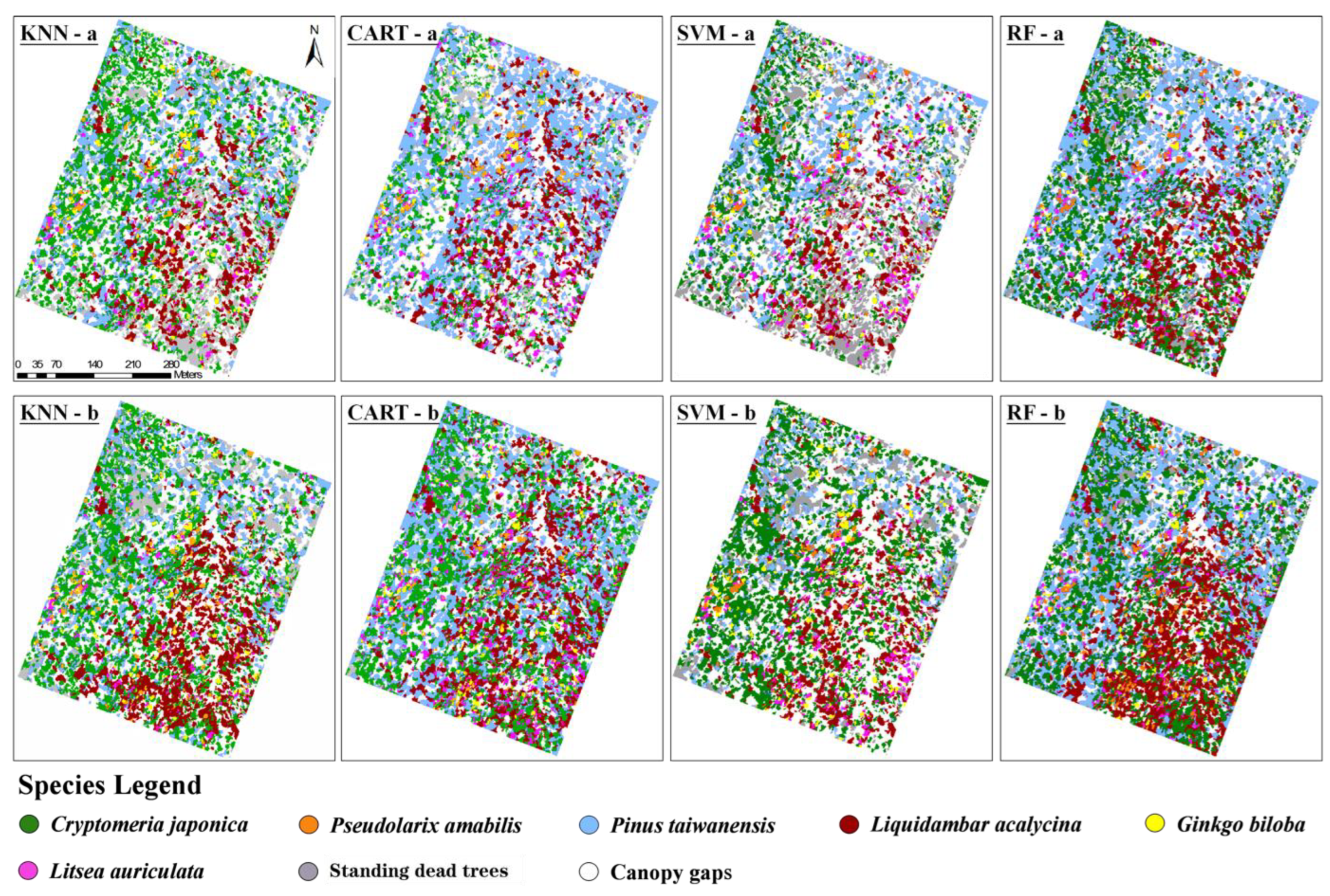
3.1. Object-Based Classification with the Combinations of Different Features

The overall accuracy of the four classification algorithms reached 68.55%–83.30% (Figure 4). Overall, Cryptomeria, Pinus, and Liquidambar were widely distributed, while Pseudolarix, Ginkgo, and Litsea were scattered within the study area or aggregately distributed in some regions (Figure 5). The maps from CART and RF contained fewer classification fragments than the KNN and SVM maps.
Among the four classification algorithms with spectral and spatial geometric features, KNN achieved the optimal accuracy of 83.30%, followed by SVM (80.70%). No matter what methods we used, Liquidambar and standing dead trees were recognized most accurately (>90% for both PA and UA) (Table 1). Among them, SVM was the best for identifying Liquidambar (PA = 97.93%, UA = 100%), and KNN for standing dead trees (PA = 100%, UA = 97.03%). The identification accuracy of other target tree species differed among the four algorithms. For example, KNN was the most accurate classifier for classifying Cryptomeria (PA = 76.05%) and Pseudolarix (60.96%), RF performed the best for identifying Pinus (82.35%) and Litsea (80.40%), and SVM performed best for Ginkgo (76.52%).
After considering texture features, the overall accuracy of RF was increased by 2.63%. The producer’s accuracy for identifying Pseudolarix increased greatly, by 22.25%, while it increased slightly for Cryptomeria and Pinus, by 6.69% and 1.37%, respectively (Table 1 and Table 2). The overall accuracy of CART was increased by 6.29%, and the producer’s accuracy of classifying Cryptomeria significantly increased, by 26.58%. On the contrary, the overall classification accuracies of SVM and KNN were reduced by 5.2% and 5.03%, and the PA and UA of almost all target tree species were reduced, especially for Pseudolarix, Pinus, Ginkgo, and Litsea (both PA and UA decreased by > 10%).
The separability among these classification objects had a marked influence on tree classification (Supplementary Table S1). Among 15 selected features, the optimal ones for tree separability were mainly composed of spectral and spatial geometry features. The top six features with high contribution were GLCM contrast, the mean value of the red band, the mean value of the green band, the mean value of the blue band, the shape index, and length/width, five of which are spectral and geometric features. Standing dead trees had the highest separability (>3.5) from other objects. The separation distances among the species with similar leaf color (e.g., Cryptomeria vs. Pinus, and Pseudolarix vs. Litsea) were relatively low, leading to misclassification when using spectral and spatial geometric features.

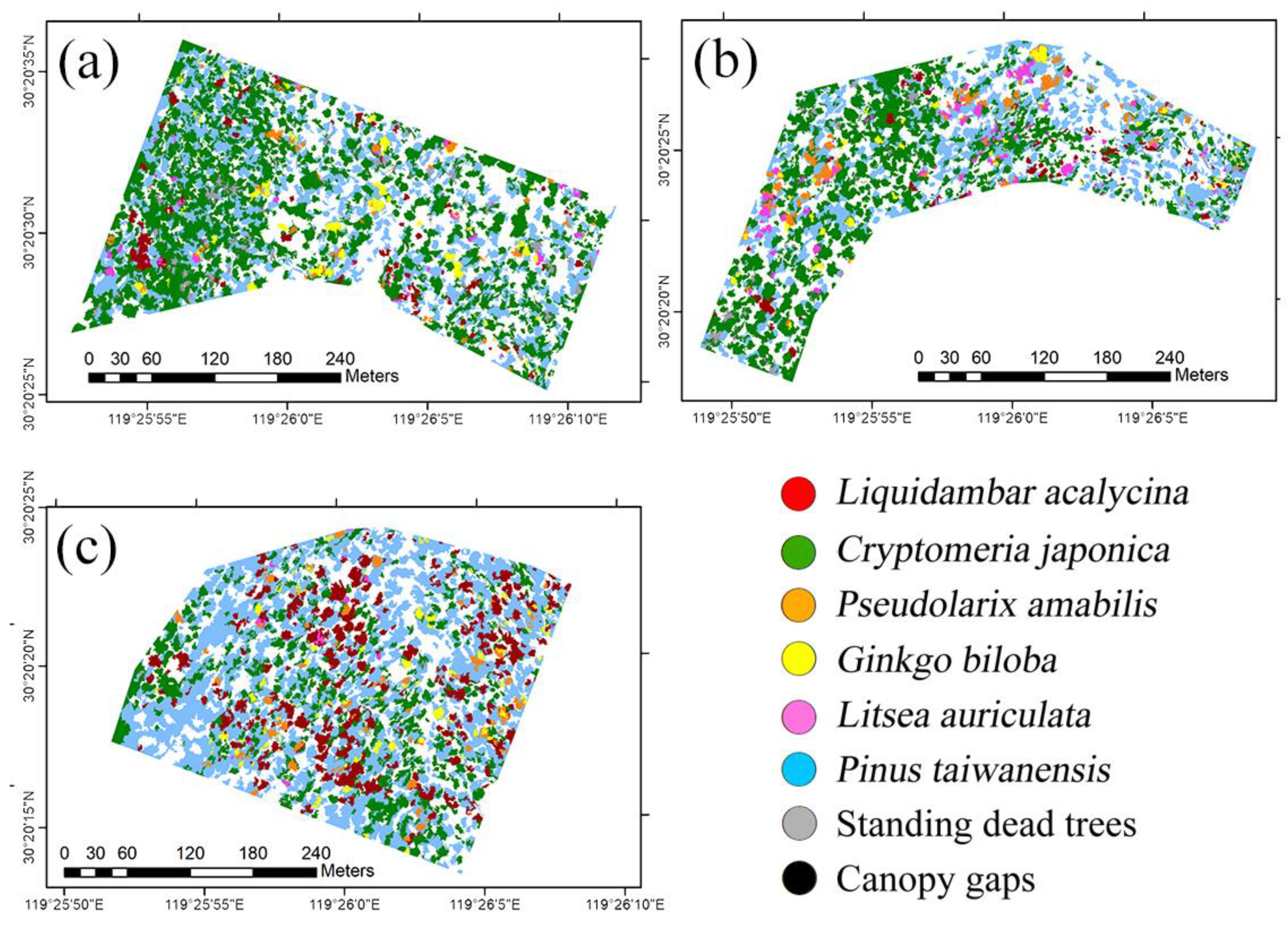
3.2. Object-Based Classification in Different Habitat Types

When we divided the study area into three habitat types (Supplementary Figure S2), different classification accuracies among the three habitats were found (Figure 6). When only using spectral and spatial geometry features, KNN had the highest classification accuracies in the upper slope (OA = 92.18%) and low slope (92.57%), and RF had the highest classification accuracy in the upper flat (82.68%). The accuracies in the upper flat and upper slope were higher than the OAs of classification without additional reference data (Supplementary Table S3). The lowest accuracy was obtained from RF in the upper slope (69.18%). After additionally considering texture features, KNN showed significantly decreased performance—the OA decreased by more than 10% in 3 habitats. SVM had more than 10% lower accuracies in the upper flat and low slope, but only 4.35% higher accuracy in the upper slope. The classifier RF slightly increased in OA, by less than 5%, in 3 habitats. Overall, the KNN with spectral and spatial geometric features performed better in most habitats than did SVM and RF (Figure 7; Table 3). Most species achieved better classification accuracies in the upper and low slopes. For example, the PAs of Cryptomeria, Pinus, Ginkgo, Liquidambar, and Litsea were obviously higher in the slope area than in the flat area, by at least 20%.
Comparing the combined map of the KNN results of three habitats (Figure 8, referred to as ‘the combined map’) and the results of the study area as a whole (Figure 9, referred to as ‘the integrated map’) with the distribution of ground samples, respectively, we found that for the tree species with a unique spectrum in the leaf senescence period (e.g., Pseudolarix, Liquidambar, Ginkgo, and Litsea), the combined map was more in line with the distribution of ground samples. The integrated map performed better for Cryptomeria and canopy gaps, since some of the patches were over-dense in the combined map. For Pinus, neither of the two maps matched the distribution of ground samples well.

4. Discussion

This study provides evidence that low-cost UAV RGB imagery from a single phenophase has great application potential in the tree species classification of species-rich montane forests. By comparing four commonly used classification methods, we found that there is no “optimal” algorithm for tree species classification, and that the performance of each algorithm may vary with features combination and tree species. When we only used spectral and spatial geometric features, the KNN (K-nearest neighbor) method is suitable for the identification of most objects (with the highest OA, and the highest PA for three tree species and standing dead trees), and SVM (support vector machine) and RF (random forest) are suitable for the identification of other three tree species and canopy gaps. After supplementing textural features, the overall classification accuracy of RF and CART (classification and regression tree) improved slightly. However, they are still inferior to the performance of KNN with only spectral and spatial geometric features. For most tree species, there was merely a seven-percent improvement of PA after adding texture information. However, for Pseudolarix amabilis and Cryptomeria japonica, the classification accuracies were improved by more than 20%. The overall classification accuracies were weakened for KNN and SVM supplementing textural features. Regarding most tree species, there was a 15%–42% decline in producer’s accuracy and a 10%–19% decline in user’s accuracy, but the computational cost increased by nearly 300 times. Overall, the textural features do not contribute much to the classification of most broadleaved tree species in our study, with two coniferous species being exceptions. This was partly in line with a study conducted in temperate forests [53] and reporting a significant role of texture features in coniferous tree species classification. In addition, some studies have also documented that texture features did not significantly improve tree species identification accuracy in pan-tropical forests [13,54]. One main reason is the high similarity in texture features among the target species from the same family or genus (e.g., Pseudolarix amabilis and Pinus taiwanensis in this study).
Compared to texture characteristics, plant spectral features of a single phenophase (leaf senescence period) play a key role in tree species classification in this study [20]. In evergreen and deciduous broad-leaved mixed forests of our study area, the proportion and composition of pigments in plant leaves during the leaf senescence period varies dramatically among tree species, resulting in leaf color differences for different tree species. These differences make the spectral features, especially the red band that corresponds to the absorption maxima of chlorophyll content [55], provide sufficient information for species classification. Species such as Pseudolarix amabilis vs. Liquidambar acalycina and Ginkgo biloba vs. Liquidambar acalycina have similar canopy shapes but varying spectrums due to different physiological and biochemical characteristics of the leaves, and therefore high separability based on spectral features. This is in line with a study classifying tree species in the Czech Republic and northwest Russia using Landsat multispectral and hyperspectral remote sensing [56]. The authors utilized tree species spectral features from multiple phenophases and found that the phenological information from the leaf (e.g., leaf unfolding in the spring and leaf fall in the autumn) was advantageous for tree species classification. Certainly, there are limitations of using data in one particular season. For example, Ginkgo biloba was less accurately identified than other species in the current study. This could be attributed to variable stages of the leaf senescence period within the species, which was probably partly related to the variation in temperature along the elevational gradient [57]. When some Ginkgo biloba were still green, others already turned yellow, resulting in various spectral signatures, which may lead to confusion in the classification. Therefore, time-series data with abundant phenological information (e.g., images in the leaf unfolding or flowering period) would be more useful in classification, especially for research on large spatial scales with more species or various forest types [20].
Topographic heterogeneity is an important factor that governs species persistence and diversification in tropical and subtropical forests by promoting the spatial turnover of plant species with different niches and providing refuge from harsh environmental conditions [58,59]. We predicted that in these species-rich forests, the species distributed in steep regions should be more difficult to identify by remote sensing data than in flat regions [60]. However, in contrast to our expectation, the classification accuracy of the steep regions was significantly higher than that of the flat regions in most instances (Figure 6). One reason is that the selection of six tree species was based on a conservation concern in addition to species dominance in the study area, and several deciduous broadleaved species (e.g., Ginkgo biloba, Liquidambar acalycina, and Litsea auriculata) were mostly distributed in habitats with complex topography such as steep slopes [61]. These species have their unique spectrums during the leaf senescence period, making them distinguishable in the slope area. In the upper flat area with relatively gentle terrain, there are fewer relict deciduous broadleaved trees, and mostly evergreen tree species such as Cryptomeria japonica and Pinus taiwanensis. Their similar spectrums in RGB bands in the sampling period made the classification difficult, despite supplementing with sufficient training samples. Multi-spectral remote sensing data would be additionally useful for accurately classifying those spectrally similar species [62]. The difference in leaf chlorophyll content can generate different spectral signals [63]; thereby Cryptomeria and Pinus should be distinguished more accurately if information on red-edge or near-infrared wavelength was available. However, adding a wavelength outside the visible spectrum means increasing the cost and difficulty of data processing. Our findings also suggest that high priority for conservation should be given to the steep area of mountains because its complex topography offers diverse microhabitats, favoring the existence of diverse plant species and preventing populations from climate change and human impacts as microrefugia [64].
Considering the influence of habitat heterogeneity on tree species classification [65], we expected that spatial distributions of tree species could be better mapped if the classifications were run in each habitat separately. The results were broadly in line with expectations. The combined maps of Pseudolarix, Liquidambar, Ginkgo, Litsea, and standing dead trees matched their distributions in the field better than for the integrated maps (Figure 8 and Figure 9). On the one hand, different topographic conditions gave the UAV images different degrees of spectral distortion. When we performed classifications in each habitat, we trained the relations between remote sensing signals and tree species and objects under similar topographic conditions, which is equivalent to excluding the influence of topography in machine learning. This demonstrates the importance of topographic influences in tree classification in mountainous forests [66,67]. On the other hand, most species that were mapped better in the combined maps were deciduous species, since they showed distinctive spectral characteristics in the leaf senescence period and were therefore easier to identify after excluding topographical influence. For the two evergreen coniferous species Cryptomeria and Pinus, due to their similar crown shapes and spectrum, identification it was still difficult even when the topographic influence was excluded.
Solid remote sensing classification cannot be carried out without enough ground reference data [68]. In our study area, due to the difference in species composition, abundance, and distributions across the whole study area and different habitats, some species in certain habitats did not provide sufficient samples. This could potentially lead to a classification bias since classification rules for predicting small classes that seldom appear are uncommon, leading to the misclassification of small classes [69,70,71]. While some species (e.g., Liquidambar and Litsea) could reach high accuracy with only five samples, some (Cryptomeria) require one hundred samples to reach the same level. In separated habitats, although we supplemented the reference data in three habitats to improve classification accuracy, the actual accuracies of some species were still relatively low, such as for Pinus and Pseudolarix in the upper flat. This may be due to the difficulty in recognizing them among the widely distributed Cryptomeria in the upper flat. Our results highlight that with sufficient ground samples, we were able to quantify the spatial variation in plant species distribution and measure its linkage with functional traits and other ecosystem functions across and within communities more accurately by establishing rigorous empirical relationships between remote sensing observation and field measurements [72,73].

5. Conclusions

In conclusion, this study showed the capability of low-cost UAV RGB imagery in the classification of subtropical montane forest species on a regional scale. In contrast to satellite remote sensing, high-resolution aerial remote sensing is capable of targeting specific times of acquisition and avoiding the impacts of cloud cover. It can greatly lower the difficulty of investigating forest resources and species distributions, especially in mountainous areas with complex terrain. In our study, the plant spectral features in the leaf senescence period play a marked role in tree species classification since subtropical montane forests feature significant species-specific spectral characteristics in this period. Our study provides a comprehensive scientific basis for a better understanding of the mechanisms of tree community assembly in species-rich subtropical forests.

Supplementary Materials

The following supporting information can be downloaded at: https://www.mdpi.com/article/10.3390/f14050908/s1, Table S1: The separations among tree species, standing dead trees and canopy gaps based on all selected features. The higher the value, the higher the separability of the two species; Figure S1: The producer’s accuracy of the classification for six tree species with different sample sizes. The x-axis on the top is for Cryptomeria japonica, and the x-axis on the bottom is for the other five species; Figure S2: (a) The maps of three topographical variables (elevation, slope, and convexity) that taken into consideration for habitat classification. Each variable was reclassified into two levels. The grid size is 30 m × 30 m. (b) The map of three habitat types produced based on the elevation and slope; Table S2: The number of samples (including ground-based and visual interpretation-based) for six target tree species, canopy gaps and standing dead trees in the (a) upper flat, (b) upper slope, and (c) low slope; Table S3: Classification accuracy of three habitat types with spectral and spatial geometric features using the KNN algorithm (without additional reference data).

Author Contributions

Conceptualization, J.Z., M.J. and J.K.; methodology, J.K., M.J. and J.Z.; software, J.K. and M.J.; validation, J.K. and M.J.; formal analysis, J.K., M.J. and Y.Q.; investigation, J.K., Z.Z., M.Z. and K.S.; data curation, J.H.; writing—original draft preparation, M.J. and J.K.; writing—review and editing, M.J. and J.Z.; supervision, J.Z.; funding acquisition, J.Z. All authors have read and agreed to the published version of the manuscript.

Funding

This research was funded by Innovation Program of Shanghai Municipal Education Commission, grant number 2023ZKZD36.

Acknowledgments

We thank Oukai Zhang and other field researchers for their assistance with field surveys and data collection. Thanks to Xin Wang and Ran Zhang for their professional suggestions. This work is part of the BEST (Biodiversity along Elevational gradients: Shifts and Transitions) research network (https://BEST-mountains.org (accessed on 24 March 2023)).

Conflicts of Interest

The authors declare no conflict of interest.

References

  1. Jetz, W.; McGeoch, M.A.; Guralnick, R.; Ferrier, S.; Beck, J.; Costello, M.; Fernandez, M.; Geller, G.N.; Keil, P.; Merow, C.; et al. Essential biodiversity variables for mapping and monitoring species populations. Nat. Ecol. Evol. 2019, 3, 539–551. [Google Scholar] [CrossRef] [PubMed]
  2. Cavender-Bares, J.; Schneider, F.D.; Santos, M.J.; Armstrong, A.; Carnaval, A.; Dahlin, K.M.; Fatoyinbo, L.; Hurtt, G.C.; Schimel, D.; Townsend, P.A.; et al. Integrating remote sensing with ecology and evolution to advance biodiversity conservation. Nat. Ecol. Evol. 2022, 6, 506–519. [Google Scholar] [CrossRef] [PubMed]
  3. FAO; UNEP. The State of the World’s Forests 2020: Forests, Biodiversity and People; FAO: Rome, Italy, 2020. [Google Scholar]
  4. Hemmerling, J.; Pflugmacher, D.; Hostert, P. Mapping temperate forest tree species using dense Sentinel-2 time series. Remote Sens. Environ. 2021, 267, 13. [Google Scholar] [CrossRef]
  5. Mayra, J.; Keski-Saari, S.; Kivinen, S.; Tanhuanpaa, T.; Hurskainen, P.; Kullberg, P.; Poikolainen, L.; Viinikka, A.; Tuominen, S.; Kumpula, T.; et al. Tree species classification from airborne hyperspectral and LiDAR data using 3D convolutional neural networks. Remote Sens. Environ. 2021, 256, 16. [Google Scholar] [CrossRef]
  6. Kim, S.; McGaughey, R.J.; Andersen, H.E.; Schreuder, G. Tree species differentiation using intensity data derived from leaf-on and leaf-off airborne laser scanner data. Remote Sens. Environ. 2009, 113, 1575–1586. [Google Scholar] [CrossRef]
  7. Franklin, S.E.; Ahmed, O.S. Deciduous tree species classification using object-based analysis and machine learning with unmanned aerial vehicle multispectral data. Int. J. Remote Sens. 2018, 39, 5236–5245. [Google Scholar] [CrossRef]
  8. Fricker, G.A.; Ventura, J.D.; Wolf, J.A.; North, M.P.; Davis, F.W.; Franklin, J. A Convolutional Neural Network Classifier Identifies Tree Species in Mixed-Conifer Forest from Hyperspectral Imagery. Remote Sens. 2019, 11, 2326. [Google Scholar] [CrossRef]
  9. Immitzer, M.; Neuwirth, M.; Bock, S.; Brenner, H.; Vuolo, F.; Atzberger, C. Optimal Input Features for Tree Species Classification in Central Europe Based on Multi-Temporal Sentinel-2 Data. Remote Sens. 2019, 11, 2599. [Google Scholar] [CrossRef]
  10. Feret, J.B.; Asner, G.P. Tree Species Discrimination in Tropical Forests Using Airborne Imaging Spectroscopy. IEEE Trans. Geosci. Remote Sens. 2013, 51, 73–84. [Google Scholar] [CrossRef]
  11. Baldeck, C.A.; Asner, G.P.; Martin, R.E.; Anderson, C.B.; Knapp, D.E.; Kellner, J.R.; Wright, S.J. Operational Tree Species Mapping in a Diverse Tropical Forest with Airborne Imaging Spectroscopy. PLoS ONE 2015, 10, 21. [Google Scholar] [CrossRef]
  12. Cross, M.; Scambos, T.; Pacifici, F.; Vargas-Ramirez, O.; Moreno-Sanchez, R.; Marshall, W. Classification of Tropical Forest Tree Species Using Meter-Scale Image Data. Remote Sens. 2019, 11, 1411. [Google Scholar] [CrossRef]
  13. Xu, Z.; Shen, X.; Cao, L.; Coops, N.C.; Goodbody, T.R.H.; Zhong, T.; Zhao, W.D.; Sun, Q.L.; Ba, S.; Zhang, Z.N.; et al. Tree species classification using UAS-based digital aerial photogrammetry point clouds and multispectral imageries in subtropical natural forests. Int. J. Appl. Earth Obs. Geoinf. 2020, 92, 14. [Google Scholar] [CrossRef]
  14. Tang, Z.Y.; Wang, Z.H.; Zheng, C.Y.; Fang, J.Y. Biodiversity in China’s mountains. Front. Ecol. Environ. 2006, 4, 347–352. [Google Scholar] [CrossRef]
  15. Zhang, J.; Hu, J.B.; Lian, J.Y.; Fan, Z.J.; Ouyang, X.J.; Ye, W.H. Seeing the forest from drones: Testing the potential of lightweight drones as a tool for long-term forest monitoring. Biol. Conserv. 2016, 198, 60–69. [Google Scholar] [CrossRef]
  16. Lisein, J.; Michez, A.; Claessens, H.; Lejeune, P. Discrimination of Deciduous Tree Species from Time Series of Unmanned Aerial System Imagery. PLoS ONE 2015, 10, 20. [Google Scholar] [CrossRef]
  17. Miyoshi, G.; Imai, N.; De Moraes, M.; Tommaselli, A.; Näsi, R. Time series of images to improve tree species classification. Int. Arch. Photogramm. Remote Sens. Spat. Inf. Sci. ISPRS Arch. 2017, XLII-3/W3, 123–128. [Google Scholar] [CrossRef]
  18. Almeida, J.; dos Santos, J.A.; Alberton, B.; Torres, R.D.; Morellato, L.P.C. Applying machine learning based on multiscale classifiers to detect remote phenology patterns in Cerrado savanna trees. Ecol. Inform. 2014, 23, 49–61. [Google Scholar] [CrossRef]
  19. Almeida, J.; Pedronette, D.C.G.; Alberton, B.C.; Morellato, L.P.C.; Torres, R.D. Unsupervised Distance Learning for Plant Species Identification. IEEE J. Sel. Top. Appl. Earth Observ. Remote Sens. 2016, 9, 5325–5338. [Google Scholar] [CrossRef]
  20. Dronova, I.; Taddeo, S. Remote sensing of phenology: Towards the comprehensive indicators of plant community dynamics from species to regional scales. J. Ecol. 2022, 110, 1460–1484. [Google Scholar] [CrossRef]
  21. Hill, R.A.; Wilson, A.K.; George, M.; Hinsley, S.A. Mapping tree species in temperate deciduous woodland using time-series multi-spectral data. Appl. Veg. Sci. 2010, 13, 86–99. [Google Scholar] [CrossRef]
  22. Persson, M.; Lindberg, E.; Reese, H. Tree Species Classification with Multi-Temporal Sentinel-2 Data. Remote Sens. 2018, 10, 1794. [Google Scholar] [CrossRef]
  23. Schriever, J.R.; Congalton, R.G. Evaluating Seasonal Variability as An Aid to Cover-Type Mapping From Landsat Thematic Mapper Data In The Northeast. Photogramm. Eng. Remote Sens. 1995, 61, 321–327. [Google Scholar]
  24. Mickelson, J.G.; Civco, D.L.; Silander, J.A. Delineating forest canopy species in the northeastern United States using multi-temporal TM imagery. Photogramm. Eng. Remote Sens. 1998, 64, 891–904. [Google Scholar]
  25. Swanson, F.J.; Kratz, T.K.; Caine, N.; Woodmansee, R.G. Landform Effects on Ecosystem Patterns And Processes. Bioscience 1988, 38, 92–98. [Google Scholar] [CrossRef]
  26. Harms, K.E.; Condit, R.; Hubbell, S.P.; Foster, R.B. Habitat associations of trees and shrubs in a 50-ha neotropical forest plot. J. Ecol. 2001, 89, 947–959. [Google Scholar] [CrossRef]
  27. Metz, M.R. Does habitat specialization by seedlings contribute to the high diversity of a lowland rain forest? J. Ecol. 2012, 100, 969–979. [Google Scholar] [CrossRef]
  28. Dong, C.; Zhao, G.X.; Meng, Y.; Li, B.H.; Peng, B. The Effect of Topographic Correction on Forest Tree Species Classification Accuracy. Remote Sens. 2020, 12, 787. [Google Scholar] [CrossRef]
  29. Yin, H.; Tan, B.; Frantz, D.; Radeloff, V.C.C. Integrated topographic corrections improve forest mapping using Landsat imagery. Int. J. Appl. Earth Obs. Geoinf. 2022, 108, 15. [Google Scholar] [CrossRef]
  30. Li, A.N.; Wang, Q.F.; Bian, J.H.; Lei, G.B. An Improved Physics-Based Model for Topographic Correction of Landsat TM Images. Remote Sens. 2015, 7, 6296–6319. [Google Scholar] [CrossRef]
  31. Tianmu Mountain Nature Reserve. Comprehensive Investigation Report on Natural Resource of Tianmu Mountain Nature Reserve; Zhejiang Science and Technology Press: Hangzhou, China, 1992. (In Chinese) [Google Scholar]
  32. Zhang, R.; Zhang, Z.C.; Shang, K.K.; Zhao, M.S.; Kong, J.X.; Wang, X.; Wang, Y.Z.; Song, H.J.; Zhang, O.K.; Lv, X.; et al. A taxonomic and phylogenetic perspective on plant community assembly along an elevational gradient in subtropical forests. J. Plant Ecol. 2021, 14, 702–716. [Google Scholar] [CrossRef]
  33. Zhou, H.Y.; Fu, L.Y.; Sharma, R.P.; Lei, Y.C.; Guo, J.P. A Hybrid Approach of Combining Random Forest with Texture Analysis and VDVI for Desert Vegetation Mapping Based on UAV RGB Data. Remote Sens. 2021, 13, 1891. [Google Scholar] [CrossRef]
  34. Stow, D.; Nichol, C.J.; Wade, T.; Assmann, J.J.; Simpson, G.; Helfter, C. Illumination Geometry and Flying Height Influence Surface Reflectance and NDVI Derived from Multispectral UAS Imagery. Drones 2019, 3, 55. [Google Scholar] [CrossRef]
  35. Whiteside, T.G.; Bartolo, R.E. A robust object-based woody cover extraction technique for monitoring mine site revegetation at scale in the monsoonal tropics using multispectral RPAS imagery from different sensors. Int. J. Appl. Earth Obs. Geoinf. 2018, 73, 300–312. [Google Scholar] [CrossRef]
  36. Blaschke, T.; Burnett, C.; Pekkarinen, A. Image segmentation methods for object-based analysis and classification. In Remote Sensing Image Analysis: Including the Spatial Domain; Jong, S.M.D., Meer, F.D.V., Eds.; Springer: Dordrecht, The Netherlands, 2004; pp. 211–236. [Google Scholar]
  37. Kamal, M.; Phinn, S. Hyperspectral Data for Mangrove Species Mapping: A Comparison of Pixel-Based and Object-Based Approach. Remote Sens. 2011, 3, 2222–2242. [Google Scholar] [CrossRef]
  38. Aguirre-Gutierrez, J.; Seijmonsbergen, A.C.; Duivenvoorden, J.F. Optimizing land cover classification accuracy for change detection, a combined pixel-based and object-based approach in a mountainous area in Mexico. Appl. Geogr. 2012, 34, 29–37. [Google Scholar] [CrossRef]
  39. Lu, D.; Weng, Q. A survey of image classification methods and techniques for improving classification performance. Int. J. Remote Sens. 2007, 28, 823–870. [Google Scholar] [CrossRef]
  40. Benz, U.C.; Hofmann, P.; Willhauck, G.; Lingenfelder, I.; Heynen, M. Multi-resolution, object-oriented fuzzy analysis of remote sensing data for GIS-ready information. ISPRS J. Photogramm. Remote Sens. 2004, 58, 239–258. [Google Scholar] [CrossRef]
  41. Cao, J.J.; Leng, W.C.; Liu, K.; Liu, L.; He, Z.; Zhu, Y.H. Object-Based Mangrove Species Classification Using Unmanned Aerial Vehicle Hyperspectral Images and Digital Surface Models. Remote Sens. 2018, 10, 89. [Google Scholar] [CrossRef]
  42. Li, L.W.; Li, N.; Lu, D.S.; Chen, Y.Y. Mapping Moso bamboo forest and its on-year and off-year distribution in a subtropical region using time-series Sentinel-2 and Landsat 8 data. Remote Sens. Environ. 2019, 231, 14. [Google Scholar] [CrossRef]
  43. Wu, S.B.; Wen, J.G.; Lin, X.W.; Hao, D.L.; You, D.Q.; Xiao, Q.; Liu, Q.H.; Yin, T.G. Modeling Discrete Forest Anisotropic Reflectance Over a Sloped Surface with an Extended GOMS and SAIL Model. IEEE Trans. Geosci. Remote Sens. 2019, 57, 944–957. [Google Scholar] [CrossRef]
  44. Haralick, R.M.; Shanmugam, K.; Dinstein, I.H. Textural features for image classification. IEEE Trans. Syst. Man Cybern. 1973, 6, 610–621. [Google Scholar] [CrossRef]
  45. Haralick, R.M. Statistical and Structural Approaches To Texture. Proc. IEEE 1979, 67, 786–804. [Google Scholar] [CrossRef]
  46. Cover, T.; Hart, P. Nearest neighbor pattern classification. IEEE Trans. Inf. Theory 1967, 13, 21–27. [Google Scholar] [CrossRef]
  47. Yang, J.M.; Yu, P.T.; Kuo, B.C. A Nonparametric Feature Extraction and Its Application to Nearest Neighbor Classification for Hyperspectral Image Data. IEEE Trans. Geosci. Remote Sens. 2010, 48, 1279–1293. [Google Scholar] [CrossRef]
  48. Breiman, L. Classification and Regression Trees; Routledge: New York, NY, USA, 1984. [Google Scholar]
  49. Vapnik, V. The Nature of Statistical Learning Theory; Springer Science & Business Media: New York, NY, USA, 1999. [Google Scholar]
  50. Gualtieri, J.A.; Cromp, R.F. Support vector machines for hyperspectral remote sensing classification. In Proceedings of the 27th AIPR Workshop: Advances in Computer-Assisted Recognition, Washington, DC, USA, 29 January 1999; pp. 221–232. [Google Scholar] [CrossRef]
  51. Breiman, L. Random forests. Mach. Learn. 2001, 45, 5–32. [Google Scholar] [CrossRef]
  52. Clark, M.L.; Roberts, D.A.; Clark, D.B. Hyperspectral discrimination of tropical rain forest tree species at leaf to crown scales. Remote Sens. Environ. 2005, 96, 375–398. [Google Scholar] [CrossRef]
  53. Shi, Y.F.; Wang, T.J.; Skidmore, A.K.; Heurich, M. Improving LiDAR-based tree species mapping in Central European mixed forests using multi-temporal digital aerial colour-infrared photographs. Int. J. Appl. Earth Obs. Geoinf. 2020, 84, 10. [Google Scholar] [CrossRef]
  54. Sothe, C.; Dalponte, M.; de Almeida, C.M.; Schimalski, M.B.; Lima, C.L.; Liesenberg, V.; Miyoshi, G.T.; Tommaselli, A.M.G. Tree Species Classification in a Highly Diverse Subtropical Forest Integrating UAV-Based Photogrammetric Point Cloud and Hyperspectral Data. Remote Sens. 2019, 11, 1338. [Google Scholar] [CrossRef]
  55. Blackburn, G.A. Spectral indices for estimating photosynthetic pigment concentrations: A test using senescent tree leaves. Int. J. Remote Sens. 1998, 19, 657–675. [Google Scholar] [CrossRef]
  56. Grigorieva, O.; Brovkina, O.; Saidov, A. An original method for tree species classification using multitemporal multispectral and hyperspectral satellite data. Silva Fenn. 2020, 54, 10143. [Google Scholar] [CrossRef]
  57. Cornelius, C.; Estrella, N.; Franz, H.; Menzel, A. Linking altitudinal gradients and temperature responses of plant phenology in the Bavarian Alps. Plant Biol. 2013, 15, 57–69. [Google Scholar] [CrossRef] [PubMed]
  58. Kallimanis, A.S.; Bergmeier, E.; Panitsa, M.; Georghiou, K.; Delipetrou, P.; Dimopoulos, P. Biogeographical determinants for total and endemic species richness in a continental archipelago. Biodivers. Conserv. 2010, 19, 1225–1235. [Google Scholar] [CrossRef]
  59. Sandel, B.; Svenning, J.C. Human impacts drive a global topographic signature in tree cover. Nat. Commun. 2013, 4, 7. [Google Scholar] [CrossRef] [PubMed]
  60. Zhang, B.; Zhao, L.; Zhang, X.L. Three-dimensional convolutional neural network model for tree species classification using airborne hyperspectral images. Remote Sens. Environ. 2020, 247, 16. [Google Scholar] [CrossRef]
  61. Shang, K.K. Differentiation Maintenance of Relict Deciduous Broad-Leaved Forest Patterns along Micro-Topographic Gradient in Subtropical Area, East China (In Chinese). Ph.D. Thesis, East China Normal University, Shanghai, China, 2011. [Google Scholar]
  62. Norton, C.L.; Hartfield, K.; Collins, C.D.H.; van Leeuwen, W.J.D.; Metz, L.J. Multi-Temporal LiDAR and Hyperspectral Data Fusion for Classification of Semi-Arid Woody Cover Species. Remote Sens. 2022, 14, 2896. [Google Scholar] [CrossRef]
  63. Cole, B.; McMorrow, J.; Evans, M. Spectral monitoring of moorland plant phenology to identify a temporal window for hyperspectral remote sensing of peatland. ISPRS J. Photogramm. Remote Sens. 2014, 90, 49–58. [Google Scholar] [CrossRef]
  64. Dobrowski, S.Z. A climatic basis for microrefugia: The influence of terrain on climate. Glob. Chang. Biol. 2011, 17, 1022–1035. [Google Scholar] [CrossRef]
  65. Giriraj, A.; Murthy, M.S.R.; Ramesh, B.R.; Dutt, C.B.S. A method for assessing evergreen habitats using phytodiversity and geospatial techniques in tropical rain forests of Southern Western Ghats (India). Ecol. Res. 2009, 24, 749–760. [Google Scholar] [CrossRef]
  66. Chiang, S.H.; Valdez, M. Tree Species Classification by Integrating Satellite Imagery and Topographic Variables Using Maximum Entropy Method in a Mongolian Forest. Forests 2019, 10, 961. [Google Scholar] [CrossRef]
  67. Hoscilo, A.; Lewandowska, A. Mapping Forest Type and Tree Species on a Regional Scale Using Multi-Temporal Sentinel-2 Data. Remote Sens. 2019, 11, 929. [Google Scholar] [CrossRef]
  68. Pau, S.; Nippert, J.B.; Slapikas, R.; Griffith, D.; Bachle, S.; Helliker, B.R.; O’Connor, R.C.; Riley, W.J.; Still, C.J.; Zaricor, M. Poor relationships between NEON Airborne Observation Platform data and field-based vegetation traits at a mesic grassland. Ecology 2022, 103, 10. [Google Scholar] [CrossRef] [PubMed]
  69. Sun, Y.M.; Wong, A.K.C.; Kamel, M.S. Classification of Imbalanced Data: A Review. Int. J. Pattern Recognit. Artif. Intell. 2009, 23, 687–719. [Google Scholar] [CrossRef]
  70. Dalponte, M.; Orka, H.O.; Gobakken, T.; Gianelle, D.; Naeesset, E. Tree Species Classification in Boreal Forests with Hyperspectral Data. IEEE Trans. Geosci. Remote Sens. 2013, 51, 2632–2645. [Google Scholar] [CrossRef]
  71. Mellor, A.; Boukir, S.; Haywood, A.; Jones, S. Exploring issues of training data imbalance and mislabelling on random forest performance for large area land cover classification using the ensemble margin. ISPRS J. Photogramm. Remote Sens. 2015, 105, 155–168. [Google Scholar] [CrossRef]
  72. Schimel, D.; Schneider, F.D.; Bloom, A.; Bowman, K.; Cawse-Nicholson, K.; Elder, C.; Ferraz, A.; Fisher, J.; Hulley, G.; Liu, J.J.; et al. Flux towers in the sky: Global ecology from space. New Phytol. 2019, 224, 570–584. [Google Scholar] [CrossRef] [PubMed]
  73. Schneider, F.D.; Ferraz, A.; Hancock, S.; Duncanson, L.I.; Dubayah, R.O.; Pavlick, R.P.; Schimel, D.S. Towards mapping the diversity of canopy structure from space with GEDI. Environ. Res. Lett. 2020, 15, 15. [Google Scholar] [CrossRef]
Figure 1. (a) The location of Mountain Tianmu, Zhejiang province; (b) the flight routes of UAV RGB image data acquisition; the small yellow planes represent take-off and landing points; (c) the UAV RGB orthoimage of the study area after pre-processing.
Forests 14 00908 g001
Figure 2. (a) The distributions of ground samples for six target tree species, standing dead trees, and canopy gaps in the study area; (b) the examples show the canopies of target tree species, standing dead trees, and canopy gaps obtained from the UAV RGB orthoimage (spatial resolution: 5 cm).
Forests 14 00908 g002
Figure 3. The examples of the image segmentation results using different parameters of scale, shape, and compactness. (a) Different scale parameters (100, 150, and 200) with default shape (0.1) and compactness (0.5); (b) different shape parameters (0.1, 0.3, and 0.5) with the “best” scale (200) and default compactness (0.5); (c) different compactness parameters (0.3, 0.5 and 0.7) with the “best” scale (200) and shape (0.3). The combination of the “best” parameters (scale: 200; shape: 0.3; compactness: 0.5) was used for the image segmentation.
Forests 14 00908 g003
Figure 4. The overall accuracy of four classification algorithms in the combinations of different features. KNN: K-nearest Neighbor; CART: Classification and Regression Tree; SVM: Support Vector Machine; RF: Random Forest.
Forests 14 00908 g004
Figure 5. The maps of tree species classification using four algorithms of the object-based classification. The letter “a” stands for the classifications based on the combinations of spectral and spatial geometric features, while “b” is for the classifications based on the combinations of spectral, spatial geometric, and textural features. Different colors represent different target objects, as shown in the legend.
Forests 14 00908 g005
Figure 6. The overall accuracy of the combinations of spectral and spatial geometry features (left panel), and spectral and spatial geometry and textural features (right panel) in three habitat types using three algorithms.
Forests 14 00908 g006
Figure 7. The maps of species classification in the (a) upper flat, (b) upper slope, and (c) low slope using KNN based on the combinations of spectral and spatial geometric features. Different colors represent different tree species as shown in the legend.
Forests 14 00908 g007
Figure 8. Spatial distributions of different species based on the KNN results of UAV imagery classification in three habitat types (the “combined map”).
Forests 14 00908 g008
Figure 9. Spatial distributions of different species based on the KNN results of UAV imagery classification across the study area (the “integrated map”).
Forests 14 00908 g009
Table 1. Classification accuracy of four algorithms with spectral and spatial geometric features.
Target ObjectsKNNCARTSVMRF
PA (%)UA (%)PA (%)UA (%)PA (%)UA (%)PA (%)UA (%)
Cryptomeria japonica76.0586.8647.9085.9666.5083.9974.0185.74
Pseudolarix amabilis60.9680.7547.1272.6459.1586.1054.4384.25
Pinus taiwanensis78.4746.6580.1729.5567.7438.2282.3546.44
Ginkgo biloba70.7165.8243.8350.1876.5264.2057.9460.23
Liquidambar acalycina97.9397.0693.8896.2797.93100.097.8290.80
Litsea auriculata63.5668.8078.3048.4269.9572.4480.4056.44
Standing dead trees100.097.0394.7993.72100.092.9895.7295.14
Canopy gaps97.8498.5082.0080.90100.094.9891.2598.38
Overall accuracy (OA, %)83.3068.5580.7080.50
Cohen’s Kappa coefficient (K)0.800.630.770.77
Table 2. Classification accuracy of four algorithms with spectral, spatial geometric, and textural features.
Target ObjectsKNNCARTSVMRF
PA (%)UA (%)PA (%)UA (%)PA (%)UA (%)PA (%)UA (%)
Cryptomeria japonica78.1676.6874.4881.9668.4875.0680.7090.53
Pseudolarix amabilis61.8066.2354.5271.9445.4081.7176.6873.10
Pinus taiwanensis45.8638.8366.8036.7825.5719.1983.7252.11
Ginkgo biloba50.8257.9651.6652.5775.5052.3156.2065.90
Liquidambar acalycina94.7397.1297.8289.4997.9399.1397.8288.83
Litsea auriculata48.4366.8054.8543.1354.6761.7463.7364.26
Standing dead trees96.0486.0689.6797.55100.097.0893.94100.0
Canopy gaps96.1295.9979.7394.0499.0392.3588.4698.33
Overall accuracy (OA, %)78.2774.8475.5083.13
Cohen’s Kappa coefficient (K)0.7360.6990.7050.798
Table 3. Classification accuracy of three habitat types with spectral and spatial geometric features using the KNN algorithm.
Target ObjectsUpper FlatUpper SlopeLow Slope
PA (%)UA (%)PA (%)UA (%)PA (%)UA (%)
Cryptomeria japonica83.8568.6710092.5710085.24
Pseudolarix amabilis29.5810043.2710076.7178.61
Pinus taiwanensis22.1340.2384.3610062.88100
Ginkgo biloba10072.6210058.0310091.39
Liquidambar acalycina10069.94100100100100
Litsea auriculata47.4959.2410010059.60100
Standing dead trees100100100100100100
Canopy gaps100100100100100100
Overall accuracy (OA, %)73.5692.1892.57
Cohen’s Kappa coefficient (K)0.6770.9020.909
Disclaimer/Publisher’s Note: The statements, opinions and data contained in all publications are solely those of the individual author(s) and contributor(s) and not of MDPI and/or the editor(s). MDPI and/or the editor(s) disclaim responsibility for any injury to people or property resulting from any ideas, methods, instructions or products referred to in the content.

