Can Wood Pellets from Canada’s Boreal Forest Reduce Net Greenhouse Gas Emissions from Energy Generation in the UK?

Abstract

We present the results of a study on the climate forcing effects of replacing coal for power generation in the United Kingdom (UK) with wood pellets produced in northern Ontario, Canada. Continuous wood pellet production from two biomass sources were considered: fiber from increased harvesting of standing live trees (stemwood scenario) and from harvest residue provided by ongoing harvesting operations (residue scenario). In both scenarios, biomass was collected from harvesting operations in two forest management units (FMUs) with contrasting harvest residue treatments: natural decay of slash piles in the Hearst FMU and slash pile burning in the Kenora FMU. Life cycle emissions associated with wood pellets were assessed for production, transportation, and combustion to replace coal at a hypothetical power generating station in the UK. Greenhouse gas (GHG) emissions and removals in wood pellet and coal scenarios were assessed using two methods: global warming potential (GWP)-based mass balance and dynamic life cycle assessment (LCA) approaches. In the stemwood scenario, climate change mitigation from replacing coal with wood pellets was not achieved within the study timeline (2020–2100). In the residue scenario, immediate climate change mitigation was achieved with fiber sourced from the Kenora FMU where the current practice is to burn slash piles; for the Hearst FMU, where slash is allowed to decompose in the forest, climate change mitigation occurred 11.6 and 3.1 years after biomass collection began, as assessed by the mass balance and dynamic LCA methods, respectively. Factors affecting mitigation potential in the studied scenarios are discussed.

1. Introduction

The continuing rise in atmospheric greenhouse gas (GHG) concentrations and the associated changes to Earth’s climate system necessitate reducing emissions and seeking opportunities to increase carbon removals from the atmosphere [1]. One such opportunity is to use forest biomass-derived energy, which is considered a renewable alternative to traditional fossil fuel-based energy sources. In 2010, the share of world primary energy consumption derived from woody biomass was estimated at about 9% and may be as high as 40% by 2050 [2]. However, not every source of forest bioenergy immediately reduces atmospheric GHGs. Consequently, rising interest in forest bioenergy has resulted in a growing number of studies assessing GHG emissions associated with producing forest bioenergy and comparing them with emissions associated with a reference energy scenario if forest biomass displaces a fossil fuel (e.g., see [3] for a review of forest bioenergy GHG accounting studies).

Not surprisingly, Canada’s vast forest resources potentially make it one of the world’s leading sources of forest biomass for energy; the IEA report [4] portrays it as “the country with the most dynamic development” in wood pellet production. According to [5], industrial wood pellet production in Canada is projected to grow from 2.9 Mt∙year⁻¹ in 2017 to 6.2 Mt∙year⁻¹ in 2030, with 83% of this production assumed to be exported. Climate change effects of using forest bioenergy produced in Canada was investigated in various studies, including differences among biomass sources such as standing live trees [6,7,8,9,10], trees harvested during commercial and pre-commercial thinning [7], salvaged dead trees [9,11], harvest residue [6,8,9,10,12,13], and mill residue [10,14]. Such studies compare the effects of bioenergy with those from using fossil fuels (coal, oil, natural gas) for local generation of heat, power, or combined heat and power (only [10,11] considered wood pellet exports to replace coal in northwestern Europe). Overall, results indicate that the time to achieve climate change mitigation increases along the progression of biomass feedstocks from residue to salvaged trees to live trees or when replacing fossil fuels associated with higher GHG emissions, from coal to oil to natural gas [9]. The overview of climate change effects for various bioenergy pathways in Canada in response to a growing demand for bioenergy was provided by [5].

The effects of Ontario-produced forest bioenergy were studied by [6,8] and also addressed in national-level studies [7,12]. The results favor the use of harvest residue-based bioenergy replacing coal-fired power, with climate change mitigation reached in year one [8] and after 16 years from the beginning of biomass collection [6]. Harvesting standing live trees required substantially longer to achieve climate change mitigation (91 years in [8] and 38 years in [6]). The elimination of coal as a fossil fuel for power generation in Ontario in 2014 has dampened local interest in forest bioenergy, since replacing oil and natural gas usually leads to much longer periods of increased GHG emissions before a mitigation benefit is obtained (e.g., [9]). However, the call for better utilization of forest resources in Ontario’s recently released forest sector strategy has revived interest in using forest biomass for energy, either locally or for export [15].

Most of the above-listed studies used a global warming potential (GWP)-based mass balance approach to assess the climate change effects of bioenergy (referred to as “100-year integrated radiative forcing using GWPs” by [16]). The GWP-based mass balance is the most frequently used approach in bioenergy studies, in which emissions and removals occurring during the study time horizon are summed regardless of when they occur [17]. The effect of non-carbon dioxide (CO₂) emissions is captured through the use of GWP, defined as the time-integrated radiative forcing due to a pulse emission of a given GHG relative to the pulse emission of an equal mass of CO₂ [16] (hence, the approach is often referred to as GWP-based). GWPs have been estimated for various periods of time, with those for 100 years commonly used to assess GHG emissions. Thus, as correctly pointed out by [14], “using this approach, the 100-year greenhouse impact is assumed to occur in the same year as the pulse emission.” To address these shortcomings, alternative assessment methods have been proposed to account for the timing of emissions and their atmospheric decay [17,18,19]. In Canada, emission timing-sensitive methods were used by [12] to assess the effects of CO₂ emissions of forest bioenergy projects. To our knowledge, ref. [14] is the only study on climate change effects of forest bioenergy in Canada that accounted for emissions of both CO₂ and non-CO₂ GHGs. Overall, despite these issues, the GWP-based mass balance approach is the predominant approach for assessing the climatic effects of GHG emissions from all sectors.

In this study, we used the life cycle analysis (LCA) to assess the climate change mitigation potential of producing wood pellets and exporting them to the UK to replace coal for power generation; the UK was chosen as it was the largest importer of Canadian-produced wood pellets [4]. We evaluated bioenergy scenarios assuming wood pellet production from either harvesting standing live trees or collecting harvest residues from two northern Ontario-forest management units (FMUs) with contrasting current management of harvest residues (slash pile burning vs. natural decay). The climate change mitigation potential of each scenario was assessed using both the traditional GWP-based mass balance approach and the radiative forcing-based approach developed by [18] (hereafter referred to as the dynamic LCA approach as used by authors). We also explore which life cycle inventory (LCI) factors affect the time to achieve climate change mitigation.

2. Materials and Methods

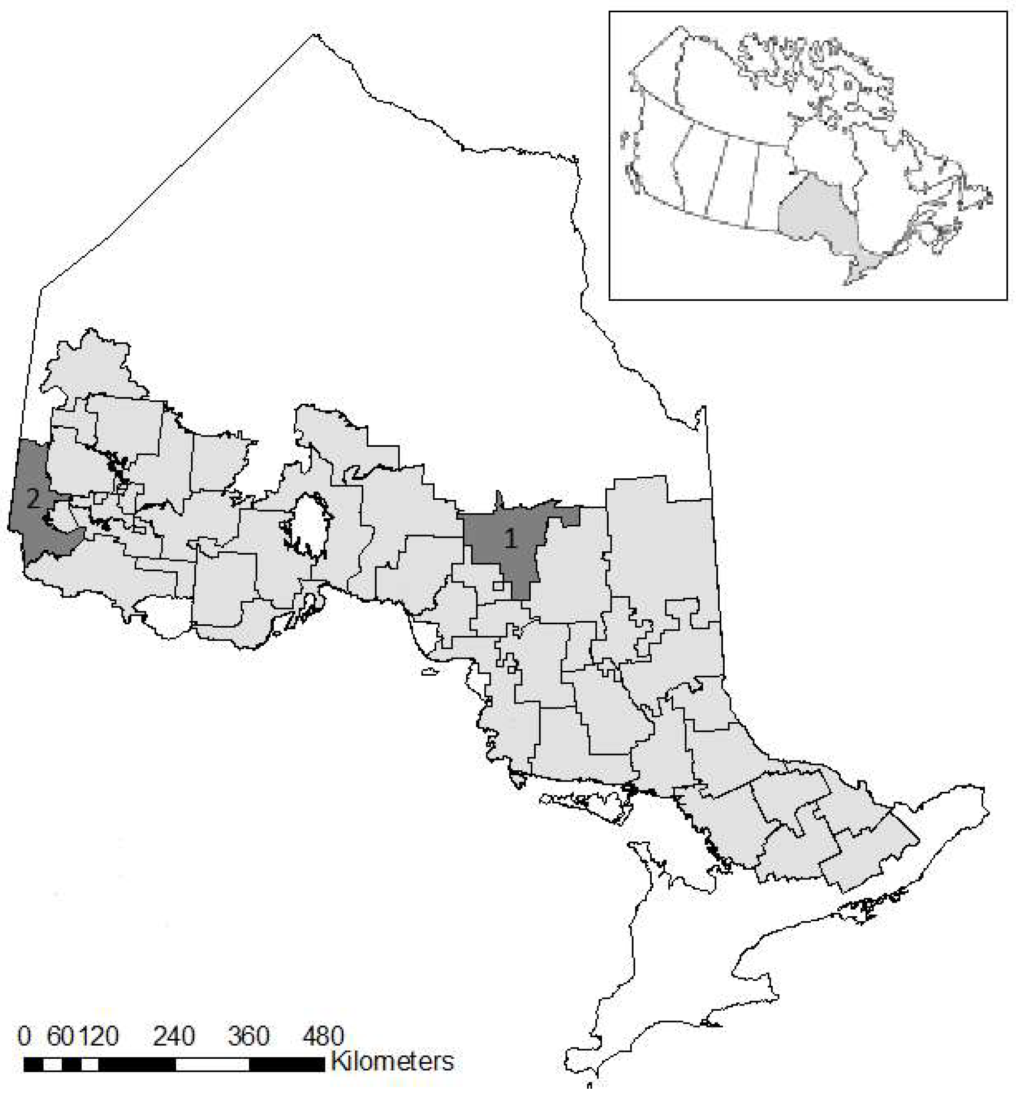
2.1. Study Area

For management purposes, forest that can be harvested in Ontario’s Crown (i.e., publicly owned) forests managed for wood production is divided into 39 (as of 2022) FMUs (Figure 1). Forestry activities in each FMU are governed by an approved forest management plan (FMP) that is updated on a ten-year cycle. FMPs and reports on completed forest operations are submitted annually and are available for public viewing (https://nrip.mnr.gov.on.ca/s/fmp-online?language=en_US, accessed on 6 November 2022). Each FMP is based on projections of forest species and ages generated using an optimization planning model: the Strategic Forest Management Model (SFMM; [20]). This model relies on forest inventory as an input and is used to simulate forest development through time based on historical natural disturbance rates, succession rules defining transition of stands from one forest type and/or age class to another, and yield curves. The model accounts for detailed silvicultural rules and prescriptions, management objectives, and environmental constraints to simulate a scenario that maximizes timber value available for harvesting.

Effects of bioenergy emissions on climate were estimated using forest biomass available for harvest in the Hearst and Kenora FMUs. These two FMUs are in the boreal zone of Ontario’s managed forest (Figure 1) and cover 1.77 million ha of forested area (1,113,000, and 652,000 ha for the Hearst and Kenora FMUs, respectively). Dominant tree species include black spruce (Picea mariana (Mill.) B.S.P.], jack pine (Pinus banksiana Lamb.), and trembling aspen (Populus tremuloides Michx.). The latest FMPs for these FMUs were approved in 2019 for Hearst and 2022 for Kenora.

2.2. Bioenergy Scenarios

Management plans for Ontario’s Crown forests managed for wood production allowed for nearly 300,000 ha to be harvested annually, although the actual harvest level averaged about 44% of this available area during 2009–2019 [21]; the rest of the available forest remains unharvested because of factors such as low market demand, cost of harvesting, and lack of access to remote stands. In the Hearst FMU, the average annual harvest volume from 1995 to 2014 was 529,720 m³ of conifer species and 56,860 m³ of hardwoods. In the Kenora FMU, harvest was 73,560 m³ of conifers and 45,250 m³ of hardwoods. The ratios of actual to available harvest volume during the same period were 0.795 and 0.297 in the Hearst FMU and 0.320 and 0.224 in the Kenora FMU for conifer and hardwood tree species, respectively. The choice of 1995–2014 as the representative period for average historical harvest is explained by [22].

In Ontario, where whole-tree harvesting is the main harvesting system, delimbing and top removal occurs at roadside [23]. The removed unmerchantable branches and tops are arranged in slash piles alongside forest access roads. In the two selected FMUs, whole-tree harvesting is used exclusively but the FMUs differ in their treatment of slash piles; in Kenora, almost all piles are burned in open fires (usually late fall–early winter), while in Hearst, slash piles are left to decay (i.e., no slash pile burning).

For each FMU, we considered two scenarios differing in the source of biomass (

Table 1. Description of bioenergy and baseline scenarios for two biomass options for two management units in northern Ontario, Canada.

FMU	Biomass	Source	Bioenergy Scenario	Baseline Scenario
Hearst Forest	Stemwood	Standing live trees from forest stands available for harvesting in the FMP but not harvested for traditional HWP.	Stands are harvested for bioenergy; harvest residue is left to decay in the slash piles at roadside.	Stands continue to develop naturally.
	Residue	Harvest residue from stands harvested for traditional HWP.	Harvest residue is collected from slash piles at roadside.	Harvest residue is left to decay in slash piles at roadside.
Kenora Forest	Stemwood	Standing live trees from forest stands available for harvesting in the FMP but not harvested for traditional HWP.	Stands are harvested for bioenergy; harvest residue is burned in the slash piles at roadside.	Stands continue to develop naturally.
	Residue	Harvest residue from stands harvested for traditional HWP.	Harvest residue is collected from slash piles at roadside.	Harvest residue is burned in slash piles at roadside.

): a stemwood scenario where trees are harvested to use merchantable parts of tree stems to produce grade A1 wood pellets, while slash is treated according to the current management practices in each FMU, and a residue scenario, in which stemwood is used for traditional wood products (e.g., construction lumber, pulp), while grade A2 pellets are produced from the biomass recovered from slash piles [24]. These scenarios represent contrasting sources of biomass for energy production: in the residue scenario, biomass is collected from existing harvest operations (i.e., no additional harvest of standing trees); in the stemwood scenario, biomass is collected from harvesting standing trees (without collecting harvest residue) in the stands identified as available for harvesting in the FMPs but remaining unharvested during ongoing harvest operations due to the above-mentioned infeasibility factors (Table 1).

Since we had no means of predicting which stands may remain unharvested, we applied the above-quoted actual-to-available harvest ratios to all stands identified in the FMPs as available for harvesting using ratios for conifers and hardwoods for stands dominated by the respective species. Forest management plans do not indicate the harvest eligibility of forest stands beyond the first 10 years of the plan. To simulate continuous harvest operations, the analysis was completed for forest stands identified for the first 10 years, and then repeated 7 times at 10 year intervals to cover the period 2020–2100 (i.e., the availability of stands for harvest during the first 10 year term was assumed to be the same in all consecutive 10 year terms).

2.3. Forest Biomass Available for Bioenergy

For management purposes, each forest stand in the FMP is identified by forest unit, silvicultural treatment, age, and net merchantable volume. Here, forest units are defined as a “classification system that aggregates forest stands for management purposes that will normally have similar species composition, will develop in a similar manner (both naturally and in response to silvicultural treatments), and will be managed under the same silvicultural system” [25]. Stand volume is estimated from yield curves included in the FMP. For each forest unit-silvicultural intensity combination, these curves specify age-specific net merchantable volume (inside bark) for each of the 16 tree species included in the standard list used to describe forest unit composition (Table S1).

Estimating the biomass available for bioenergy for each stand identified as available for harvesting in the FMPs included the following steps. In the stemwood scenario, available biomass B_stem was estimated by converting tree volumes into units of mass and adding the mass of tree bark:

$$B_{stem}=V·Dens·\left(1+Fra{c}_{bark}\right)$$

(1)

where B_stem (odt∙ha⁻¹) is the biomass of the merchantable part of the stem (with bark) in oven-dried metric tons per hectare, V (m⁻³∙ha⁻¹) is the inside-bark volume of the merchantable part of the tree stem, Dens (t∙m⁻³) is the average tree stem density per unit of green volume, and Frac_bark is the ratio of stem bark mass to stem mass.

In the residue scenario, available biomass B_res was calculated by (a) estimating the total aboveground biomass of a stand, (b) subtracting foliage biomass, (c) subtracting biomass in merchantable stems with bark, (d) dividing slash biomass estimated in steps (a)–(c) between biomass left on the harvested site and that in roadside slash piles, and estimating the fraction of roadside slash piles that is technically and economically recoverable:

$$B_{res}=\left[B_{Ag}·\left(1-Fra{c}_{fol}\right)-B_{stem}\right]·\left(1-Fra{c}_{site}\right)·Fra{c}_{recovery}$$

(2)

where B_res (odt∙ha⁻¹) is the biomass of unmerchantable parts of stem per unit of harvest area available for wood pellet production, B_Ag (odt∙ha⁻¹) is the total aboveground biomass of live trees, Frac_fol is the ratio of foliage mass to total aboveground biomass of live trees, Frac_site is the fraction of unmerchantable tree biomass left scattered on site during whole-tree harvesting, and Frac_recovery is the fraction of unmerchantable biomass in slash piles at roadside that can be recovered to produce wood pellets. The quantities B_stem, B_res, and B_Ag and V are per unit of harvest area; V and Dens are species-specific, Frac_bark and Frac_fol are species-type specific (conifers or hardwoods), while Frac_site and Frac_recovery are applied to all species. How the above-listed quantities were estimated is described below.

The stem biomass of each species included in the forest unit yield was calculated using stemwood densities, Dens, from [26]; see the Supplementary Materials. To estimate the amount of foliage and stem bark, we used individual tree measurements from the growth sample plots established within the framework of Ontario’s Growth and Yield Program [27,28]. The plot-level ratios of foliage biomass to total aboveground biomass (Frac_fol) and of stem bark to stem wood biomass (Frac_bark) were estimated separately for conifer- and hardwood-dominated plots by summing foliage and bark biomass of individual trees estimated using DBH-based allometric equations from Lambert et al. [29]. The estimated ratios were plot age-independent for conifer-dominated plots while for hardwood-dominated plots, age-dependence was modelled using negative exponential function (see the Supplementary Materials).

The amount of total aboveground biomass of live trees was estimated using equations from the FORCARB-ON2 model [30,31]; the model is described in Section 2.5. We followed the approach used in FORCARB-ON2 to estimate aboveground biomass using volume densities for the following species groups: P—jack, red, and white pine; SF—black and white spruce and fir; AB—aspen-birch; and MB—maple-beech. Each of the 16 major Ontario tree species represented in the standard forest units were assigned to one of the species groups (P, SF, AB, or MB); in addition to the above listed tree species, eastern white cedar, hemlock, and “other conifers” were assigned to the SF group, balsam poplar to AB, and red oak and yellow birch to MB (see the Supplementary Materials for scientific names of tree species). The species group volume density (m³ ha⁻¹) was estimated as the sum of net merchantable volumes for individual species in the group divided by the fraction of the species group volume in the total stand volume. The species group volume density was converted to aboveground biomass of live trees using FORCARB-ON2 equations, and the resulting estimates were summed to provide stand totals weighted by the fraction of a species group’s volume in total stand volume.

The fraction of unmerchantable biomass left on site in whole-tree harvesting operations was assessed in various studies, either by means of direct measurements of biomass left on site and at roadside (e.g., [23]), or by comparing the amounts of unmerchantable biomass left on site in whole-tree and stem-only harvesting operations (e.g., [32,33]). In the latter studies, the amount of coarse and fine woody debris in control plots was deducted from that in whole-tree and stem-only harvested plots to remove the “background” level of biomass present in plots regardless of harvesting operations. Closest to our study conditions are the findings by [23], who estimated the amount of slash left on harvesting sites and at roadside at three sites in northern Ontario. Using their results, we calculated the fraction of unmerchantable biomass left on site to be 0.56 for an upland mixed-wood stand (49% softwood and 51% hardwood), 0.69 for an upland mixed-wood stand with slightly more conifers (50% conifer and 41% hardwood), and 0.35 for a pure lowland black spruce stand. These fractions were calculated using estimates of slash obtained during field measurements, not those predicted by the model tested by [23]. The estimated fractions align with those reported by [32,33], who estimated the fraction of unmerchantable biomass left on site at 0.46 and 0.52 for aspen-dominated stands in Quebec, Canada, and hardwood stands in Minnesota, USA, respectively. A similar fraction (0.56) was estimated by [34] in thinning studies in conifer stands in Finland. Finally, leaving half of the residue on site is also recommended by [35] for ecological reasons. Based on all these results, we chose 0.50 for Frac_site in Equation (2), i.e., the fraction of unmerchantable biomass left on the harvesting site.

Finally, to estimate the biomass available for wood pellet production, the amount of biomass in slash piles at roadside (estimated with the above-described fraction of unmerchantable biomass left on site) must be multiplied by the faction of biomass that can be recovered from slash piles at roadside. We used 0.75 for the latter fraction, Frac_recovery, based on results from [23]. In that study, the fraction of recoverable biomass at three sites was estimated to be 0.13, 0.78, and 0.77. We ignored the first estimate since, as noted by the authors, at that site, “the residues were older and more contaminated than on the other blocks, which limited the recovery to only hardwood tops and branches.”

2.4. Analysis Framework

Two methods were used to assess climate change effects of the two bioenergy scenarios: the GWP-based mass balance approach to assess the time needed to achieve carbon neutrality (carbon sequestration parity) and the dynamic LCA approach to assess the time needed to achieve climate neutrality. Descriptions of both approaches are as follows.

2.4.1. GWP-Based Mass Balance Approach

For the GWP-based mass balance approach, we used the analysis framework developed by [6,8]. The framework combines an LCI analysis to quantify GHG emissions from energy produced using forest biomass and forest carbon modelling to quantify the effect of biomass harvest on forest carbon stocks over time. The life cycle inventory analysis includes GHG emissions related to all phases of producing energy from forest biomass, such as collecting biomass (standing tree harvest or collection of harvest residue), regenerating harvested stands, constructing and maintaining roads, transporting biomass to the pellet facility, pelletizing, transporting pellets to the generating station, and using biomass in place of fossil fuels. Changes in forest carbon stocks with and without biomass harvest for bioenergy are modelled separately and therefore are not included in the LCI. Total GHG emissions equal the sum of contributions to GHG emissions resulting from the LCI and from changes in forest carbon stocks.

For a one-time forest biomass harvest occurring at time T₀, total GHG emissions at time t after harvest (GHG_Total; t CO₂eq, tonnes of CO₂ equivalent) can be calculated as:

$$GH{G}_{Total}\left(T_0+t\right)=\Delta FC\left(T_0+t\right)+Z\left(T_0\right)·P_{Bio}·\left(GH{G}_{LCAbio}-GH{G}_{LCAfossil}\right)$$

(3)

where ΔFC is change in forest carbon resulting from biomass harvest (t CO₂eq), Z(T₀) is the amount of biomass harvested to produce energy (odt, oven-dry tonnes) at time T₀, P_Bio is the energy produced by one odt of biomass (MWh∙odt⁻¹), GHG_LCAbio is life cycle emissions from producing forest biomass energy (t CO₂eq∙MWh⁻¹) but excluding CO₂ emissions from biomass combustion, and GHG_LCAfossil is life cycle emissions from producing the same amount of energy using fossil fuels (t CO₂eq MWh⁻¹). GHG variables in Equation (3) are presented in tons of CO₂ equivalent—CO₂eq (one ton of carbon is equivalent to 3.667 tons of CO₂) to account for non-CO₂ GHG emissions, which require conversion into CO₂eq using 100-year GWP multipliers. To express changes in forest carbon stocks in the same units as GHG emissions, ΔFC was also converted to t CO₂eq. The difference (GHG_LCAbio—GHG_LCAfossil) is the GHG emission benefit of producing one unit of energy from forest biomass instead of fossil fuels, while the entire second term in Equation (3) is the total GHG emissions benefit from using Z(T₀) biomass instead of fossil fuels.

Change in forest carbon resulting from biomass harvest (ΔFC) equals the difference between forest carbon stocks after biomass harvest and those in the baseline scenario (if there was no biomass harvest for energy):

$$∆FC\left(T_0+t\right)=F{C}_{base}\left(T_0+t\right)-F{C}_{bio}\left(T_0+t\right)$$

(4)

Here, FC_bio(T₀ + t) is forest carbon stock (t CO₂eq) at time t after biomass harvest and FC_base(T₀ + t) is forest carbon stock (t CO₂eq) at time t if residues were not collected (residue scenario) or stands were not harvested (stemwood scenario) for bioenergy. For continuous biomass harvest to produce energy, Equation (3) is integrated over time starting from the first year of biomass harvest for both residue and stemwood scenarios. Time t after the beginning of biomass harvest, at which GHG_Total in Equation (3) becomes zero, is called time to carbon sequestration parity or time to carbon neutrality. It reflects the time needed for the GHG benefits of displacing fossil fuels with biomass to offset forest carbon losses, accounting for changes in forest carbon that would have occurred in the absence of biomass harvest.

The amount of energy produced from one odt of biomass, P_Bio, can be calculated as:

$$P_{Bio}=\left(1-Los{s}_{Bio}\right)·NC{V}_{WP}·E{E}_{Bio}$$

(5)

where Loss_Bio is the fraction of biomass lost along the supply chain, partly during transportation from the forest to the power plant but mostly due to its use to generate heat for drying the biomass at the pelletization plant to reduce wood moisture content (odt∙odt⁻¹); NCV_WP is the net calorific value of wood pellets (MWh∙odt⁻¹); and EE_Bio is the electrical efficiency of the biomass power plant (MWh∙MWh⁻¹). Following [8], we used 0.15 for Loss_Bio. The net calorific value is from [36] who estimated an average low heating value at 5.31 MWh∙odt⁻¹ (19.09 TJ∙Gg⁻¹) in a study of wood pellets from eight Canadian producers; the lower heating value was chosen because according to [37], “in the European practice efficiency calculations are based on low heating value.” For plant efficiency, usually defined as the electric energy output as a fraction of the fuel energy input of a thermal power plant [37], we used 0.38, which is the efficiency of one of the units in a Drax power plant in the UK [38]. Altogether, these estimates resulted in P_Bio being equal to 1.715 MWh∙odt⁻¹.

2.4.2. Dynamic LCA Approach

The dynamic LCA approach follows the methodology by [18] who developed instantaneous dynamic characterization factors (DCF) for the global warming impact assessment of GHG emissions. Levasseur et al. [18] defined instantaneous DCF for the time interval (t − 1,t) after emission of a given gas i at time 0 as:

$$DC{F}_i\left(t\right)={{\displaystyle \int }}_{t-1}^{t}IR{F}_i·C_i\left(t\right)dt$$

(6)

where IRF_i is the instantaneous radiative forcing per unit mass increase of gas i in the atmosphere and C_i(t) is the time-dependent atmospheric load of the released gas i; three gases considered in such analyses are carbon dioxide (CO₂), methane (CH₄), and nitrous oxide (N₂O). The instantaneous global warming impact (GWI_inst) at time t of all releases of the three GHGs is calculated as:

$$\begin{gathered} GW{I}_{inst}\left(t\right)={\displaystyle \sum }_{j=0}^t\left(g_{C{O}_2}\left(j\right)·DC{F}_{C{O}_2}\left(t-j\right)+g_{C{H}_4}\left(j\right)·DC{F}_{C{H}_4}\left(t-j\right)+g_{N_{2}O}\left(j\right) \\ ·DC{F}_{N_{2}O}\left(t-j\right)\right) \end{gathered}$$

(7)

where g_CO2(j), g_CH4(j), and g_N20(j) are emissions of CO₂, CH₄, and N₂O at time j. In other words, the global warming effect of gas i at time t reflects the radiative forcing effect of all emissions of gas i that occurred from time 0 to t. Consequently, the cumulative global warming impact (GWI_cum) at time t is the sum of all instantaneous global warming impacts between 0 and t:

$$GW{I}_{cum}\left(t\right)={\displaystyle \sum }_{i=0}^{t}GW{I}_{inst}\left(i\right)$$

(8)

For CO₂, the atmospheric load C_CO2(t) following a pulse emission is given by the Bern carbon cycle-climate model:

$$C_{CO2}\left(t\right)=a_0+{\displaystyle \sum }_{i=1}^3{a}_i·\exp \left(-\frac{t}{{\tau }_i}\right)$$

(9)

where a₀ = 0.2173, a₁ = 0.2240, a₂ = 0.2824, a₃ = 0.2763, τ₁ = 394.4 years, τ₂ = 36.54 years, and τ₃ = 4.304 years [39]. For CH₄ and N₂O, the atmospheric load C(t) following a pulse emission is given by a first-order decay equation where the inverse of the kinetic constant is the adjusted lifetime τ:

$$C\left(t\right)=\exp \left(-\frac{t}{\tau }\right)$$

(10)

where τ_CH4 = 12.4 years and τ_N2O = 121 years [39].

To estimate instantaneous and cumulative global warming impacts for bioenergy and baseline scenarios, changes in forest carbon stocks defined in Equations (3) and (4) must be annualized (i.e., presented as a series of one-year-long emissions and removals of forest carbon) for each scenario and combined with the annual life cycle emissions of each of the three GHGs (excluding CO₂ emissions from biomass combustion). When calculating global warming impacts, reductions (emissions) and increases (removals) in forest carbon stocks are included in Equation (7) with positive and negative signs, respectively. Time t after the beginning of biomass harvest, at which global warming impacts of bioenergy and respective baseline scenarios (GWI_cum(t) calculated using Equation (3)) are equal, is called time to climate impact neutrality (i.e., time to achieve climate change mitigation benefits of using bioenergy).

2.5. Changes in Forest Carbon Stocks

Changes in forest carbon stocks in stemwood and corresponding baseline scenarios were simulated using FORCARB-ON2, the Ontario adaptation of the forest carbon budget model FORCARB2 [31,40]. FORCARB2 was developed by the USDA Forest Service and used to generate regional and national-scale estimates of carbon stocks in U.S. forests and harvested wood products. The Ontario version of the model followed the same structure as the original model, but with added modules to simulate the effects of fire disturbance, carbon conversion among forest carbon pools, and dynamics of dead biomass and soil carbon pools; relevant parameter values were modified to better reflect local forest conditions [40]. FORCARB-ON2 has been used in numerous applications to estimate current carbon stocks and to predict future carbon stocks in forests and harvested wood products at forest management units and provincial scales for various forest management scenarios [30,41,42].

FORCARB-ON2 provides estimates of forest ecosystem carbon stocks in six pools: live trees (above- and belowground), standing dead trees (above- and belowground), down dead wood (DDW, which includes logs and branches ≥76 mm in diameter as well as stumps), understory vegetation, forest floor (dead organic matter above the mineral soil horizon, including branches and logs <76 mm in diameter, litter, and humus), and soil [30]. Carbon stocks in various pools were derived using relationships with net stand merchantable volume (for carbon in live and standing dead trees), with live tree biomass (for DDW), with stand age (for forest floor and understory vegetation), or with forest type (for soil). These relationships were based on regression equations developed using the USDA Forest Service’s Forest Inventory and Analysis database [43] and were designed to describe the average carbon stocks in forest stands of a given species composition and age. Unlike the original model, FORCARB2, in FORCARB-ON2 carbon stocks in dead organic matter pools (standing dead trees, down wood, forest floor, and soil) are simulated using the processes of transition among various pools and the decomposition of the pool content from the previous simulation step.

FORCARB-ON2 was used to estimate forest carbon stocks:

In the stemwood scenario (both FMUs), for pre-harvest stocks in areas identified as available for harvesting, followed by harvesting and regeneration;

In the baseline to stemwood scenario (both FMUs), for dynamics of stocks in areas identified as available for harvesting (natural growth in the absence of harvesting);

In the stemwood scenario (Hearst FMU), for stocks in forest regenerating in areas covered with slash piles produced during harvesting and then cleared due to slash decay;

In the stemwood scenario (Kenora FMU), for stocks in forest regenerating in areas covered with slash piles produced during harvesting and cleared due to slash pile burning;

In the residue scenario (Hearst FMU), for stocks in forest regenerating in areas covered with slash piles and cleared due to slash collection for bioenergy;

In the baseline to residue scenario (Hearst FMU), for stocks in forest regenerating in areas covered with slash piles produced during harvesting and then cleared due to slash decay.

Simulations were conducted for forest areas identified as available for harvesting in the FMPs that were projected to stay unharvested based on the FMU-specific historic ratio of actual-to-available harvest (see Section 2.1); the ratios were applied separately to conifer- and hardwood-dominated forests. The areas covered with slash piles were estimated using an FMU-specific ratio of slash pile-to-harvest area (to simulate regeneration due to slash pile decay, burning, or collection). Forest growth, both in unharvested and regenerating areas, followed the same rules (growth and yield curves, natural disturbance rates, successional transition rules, and post-harvest and post-disturbance transitions) as those used to develop the FMPs (see Section 2.1). Note that carbon stocks with an identical fate in bioenergy and baseline scenarios were not included in the simulations because these stocks would cancel each other out in scenario comparisons.

The fate of carbon stocks in slash piles was simulated following the approach used by [8,44]. For the Hearst FMU, the decay of mass in slash piles in the absence of collection for bioenergy was simulated using a negative exponential function, with all emissions in the form of CO₂. Following [44], we used decay rates of 0.0171 year⁻¹ and 0.0365 year⁻¹ for conifers and hardwoods, respectively. The selected decay rates resulted in a 50% loss of pile mass by years 41 and 19 for pure conifer and pure hardwood slash, respectively; decay losses in simulated slash piles were dictated by the fractions of conifer and hardwood unharvested biomass mass left at roadside in slash piles, as described in Section 2.3.

In the Kenora FMU, the current management practice is the burning of all slash piles generated during harvesting. In the harvest residue scenario, combustion emissions were not explicitly simulated because it was assumed that burning biomass either in the form of slash piles or wood pellets results in the same emissions, cancelling each other in scenario comparisons. In the stemwood scenario, slash pile combustion was assumed to be 0.88 efficient [44,45]; the unburned fraction of slash piles was assumed to decompose as described above. The combusted fraction of slash piles produces black carbon, a product of incomplete combustion that includes char, ash, and charcoal and resists further biological or chemical degradation; the amount of black carbon produced during slash pile burning was estimated to be 0.0225 of the combusted carbon. Gaseous emission factors from the rest of the combusted biomass were estimated as 1.55550, 0.00805, and 0.00011 tonnes∙odt⁻¹ for CO₂, CH₄, and N₂O, respectively [46], based on emissions from boreal forest wildfires. In the GWP-based mass balance approach, CH₄ and N₂O emissions were converted into CO₂eq using global warming potential factors of 27.9 and 273.0, respectively, estimated over 100 years [47]. In the dynamic LCA, the contribution of non-CO₂ emissions to radiative forcing was estimated using the methods described in Section 2.4.2.

Finally, the regeneration of areas recovered due to slash pile decay (upon decay losses reaching 50% of the initial slash pile biomass) and burning was simulated using average post-harvest regeneration rates for respective FMUs. The area covered with slash piles was estimated at 0.03 and 0.025 of the total harvested area as per FMPs for the Hearst and Kenora FMUs, respectively; the fraction of area covered with slash piles in the Hearst FMU was taken as the average of observed (0.042) and projected (0.02) fractions.

2.6. LCI Emissions

LCI emissions in bioenergy scenarios were estimated for the following activities: biomass harvesting and harvest residue collection (in stemwood and residue scenarios, respectively), forest renewal, forest road construction, biomass transportation to a pellet facility, pelletization, and pellet delivery to a generating station in Selby, UK. It was assumed that in both FMUs, biomass was trucked to a pellet manufacturing facility an average distance of 100 km. After production and packaging, wood pellets are transported from the plant to Halifax (Nova Scotia, Canada) port by train, a total distance of 2800 km and 3800 km from the Hearst and Kenora FMUs, respectively. In Halifax, the wood pellets are loaded on ocean vessels and shipped to Liverpool (UK), a distance of about 4550 km, and then transported by train to Selby. All transportation distances were estimated using Google Maps; total transportation distances by train were rounded to 3000 and 4000 km for wood pellets originating from the Hearst and Kenora FMUs, respectively.

Emissions for LCI phases were based on estimates derived by [48,49,50]. Since wood pellets are not currently produced in either FMU, it was assumed that pelletization plants are built in both Hearst and Kenora. The LCI emissions from construction of pelletization plants with a life span of 40 years were taken from [8] and were all assumed to occur in the first year of biomass collection for bioenergy; thus, for continuous harvest operations the emissions from construction of pelletization plants were simulated in years 1 and 41 from the start of collecting biomass for energy. With the exception of the harvest residue scenario in the Kenora FMU (in which biomass was assumed to be burned in both bioenergy and baseline scenarios), LCI for wood pellets also included non-CO₂ emissions from biomass combustion using emission factors from [51]; CO₂ combustion emissions were not included to avoid double-counting, since these emissions are already accounted for as carbon losses during harvesting and slash pile collection. For a detailed breakdown of LCI emissions, see Table S2 in the Supplementary Materials.

Finally, LCI emissions from using coal as a fossil fuel were taken from [52]. Total LCI emissions for two biomass and coal scenarios are presented in

Table 2. Total life cycle inventory emissions (kg∙MWh⁻¹) for bioenergy and coal scenarios for two forest management units in northern Ontario, Canada; emissions for bioenergy scenarios do not include those from pellet plant construction.

Gas, kg∙MWh−1	Hearst FMU		Kenora FMU		Coal Scenario
	Stemwood Scenario	Residue Scenario	Stemwood Scenario	Residue Scenario
CO2	119.975	78.476	126.220	84.721	875.0
CH4	0.227	0.202	0.233	0.100	2.90
N2O	0.038	0.027	0.040	0.015	0.06

; the LCI emissions for the biomass scenarios do not include emissions from construction of pellet plants that are equal to 22.18, 0.0019, and 0.00031 tons of CO₂, CH₄, and N₂O, respectively, that occur once every 40 years.

2.7. Sensitivity Analysis

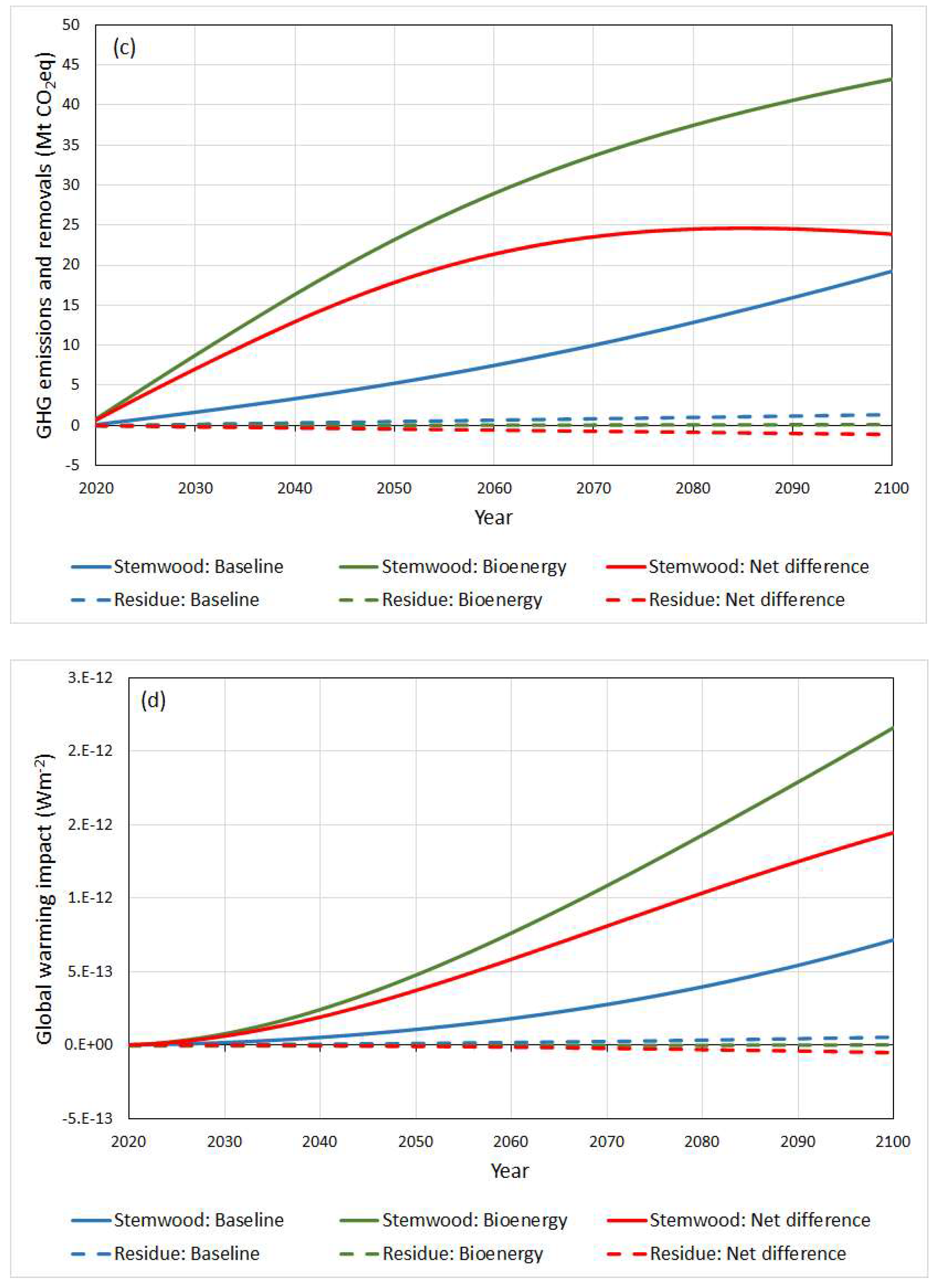
A sensitivity analysis was used to test robustness of assessed GHG emissions and global warming impact factors for bioenergy scenarios to assumptions and LCI estimates. To explore the effects of LCI emissions, we used a set of hypothetical scenarios, each with the emissions for one or more of the LCI phases in the bioenergy scenario set to zero (e.g., no emissions from train or sea vessel transportation, etc.). To test the effect of tree growth rate on total GHG emissions in the stemwood scenario, we modified yield curves to simulate the accelerated accumulation of carbon stocks in post-harvest regenerating stands (i.e., effect of more rapid regeneration and early growth rates). We followed the approach used by [8], (a) retaining maximum carbon stocks in live trees and changes to these stocks past the age at which the maximum was reached and (b) shifting to the left the part of live tree carbon curve from age zero to the maximum age by proportionally reducing the years needed to reach the maximum by a factor of two. The resulting curve was equivalent to doubling the rate of carbon stock accumulation in live trees of regenerating stands while leaving the stocks intact past the point of maximum accumulation.

3. Results

In the stemwood scenario, the amount of biomass that could be harvested for wood pellet production in the Hearst FMU contains an estimated 27,100 and 34,030 tC∙year⁻¹ in conifer- and hardwood dominated blocks, respectively. In the Kenora FMU, the respective amounts were 23,220 and 42,950 tC∙year⁻¹. As per scenario assumptions, these estimates reflect the amount of biomass harvestable from stands not harvested for traditional HWP. In the residue scenario, the amount of biomass in roadside slash piles contained 61,110 and 7150 tC∙year⁻¹ in the Hearst FMU and 5870 and 7140 tC∙year⁻¹ in the Kenora FMU in conifer- and hardwood dominated blocks, respectively. Contrary to the stemwood scenario, the biomass in residue is obtained from stands harvested for traditional HWP, regardless of pellet production.

Results of the scenario comparisons are presented in Figure 2; an alternative grouping of the emissions and removals is presented in Figure S2. As evident in Figure 3, cumulative emissions and global warming impacts from the use of stemwood for pellets in both FMUs outweigh those in the baseline scenario for more than the next 80 years, i.e., no climate change mitigation benefit is evident by 2100 from replacing coal with the wood pellets produced from harvesting standing live trees. In contrast, using harvest residues for pellets, carbon sequestration parity is achieved after 11.6 years from the beginning of pellet production in the Hearst FMU, while in the Kenora FMU, it is achieved in the first year; using the dynamic LCA approach, the time to climate impact neutrality was 3.1 and less than 1 year(s) for the Hearst and Kenora FMUs, respectively.

Results of testing the effects of emissions for individual LCA phases and regeneration rates on cumulative GHG emissions in stemwood versus baseline scenarios are presented in Figure 3 For the Hearst FMU, assuming that all GHG emissions associated with producing and transporting wood pellets equal zero (including non-CO₂ combustion emissions) reduced the difference in cumulative emissions and removals between stemwood and baseline scenarios by 5.7% and 8.6% by years 2050 and 2100, respectively. The respective reductions for the Kenora FMU were 3.7 and 7.2%. Obviously, the effect was even smaller when setting emissions from individual LCA phases to zero (not shown). The effects were of similar magnitude when using the dynamic LCA assessment method. In the harvest residue scenario, setting all LCA emissions associated with wood pellet production in the Hearst FMU to zero lowered the time to carbon sequestration parity to 5.3 years, while climate impact neutrality was achieved in the first year.

As shown in Figure 3, doubling the rate of carbon accumulation in stands regenerating after harvest had a noticeable effect on the cumulative difference in GHG emissions and removals between the stemwood and its baseline scenarios, reducing them by 37.1% by 2050 and 53.6% by 2100 for the Hearst FMU; for the Kenora FMU, respective reductions were 23.1% and 42.5%. However, the simulated increase in regeneration rates was insufficient to achieve either carbon sequestration parity or climate impact neutrality in the stemwood scenario within the study time frame.

4. Discussion

Our analyses indicate that producing wood pellets from harvesting standing live trees in two FMUs in northern Ontario and shipping these pellets to the UK to replace coal for power generation does not mitigate climate change within the 80-year time frame of this study (year 2100). In comparison, a climate change mitigation benefit from replacing coal with Ontario-produced wood pellets occurs if the pellet feedstock is harvest residue left at roadside during harvesting operations for traditional HWP. The time to achieve a climate change mitigation benefit from the beginning of biomass collection depends on harvest residue practices in the baseline scenario, ranging from zero years in the Kenora FMU where slash pile burning is practiced for several years in the Hearst FMU where slash piles are left to decay. Similar results are obtained with both assessment methods, differing only in the time needed to achieve a climate change mitigation benefit with harvest residue in the Hearst FMU (11.6 and 3.1 years from the beginning of residue collection using mass balance and dynamic LCA approaches, respectively).

Our assessment of climate change mitigation potential is consistent with previously published results for the two studied bioenergy scenarios, with the mitigation benefit achieved in the short-term for the residue collection scenario but taking decades when standing live trees are harvested. For example, in a Canada-wide study, Smyth et al. [7] found no climate change mitigation benefit within their study time frame (35 years) when bioenergy produced from either additional clear-cut harvest or increased pre-commercial and commercial thinning was used to displace a locally specific mix of energy sources. Ter-Mikaelian et al. [8] concluded that harvesting standing live trees for wood pellets in northwestern Ontario, Canada, to replace coal at a local coal-fired generating station, required 91 years from the beginning of harvesting to achieve a mitigation benefit. Using growth curves typical of forest regeneration rates in Canada, Laganière et al. [9] estimated it would take longer than 120 years to achieve benefits when bioenergy from harvesting standing live trees replaced any of the main fossil fuels (coal, oil, natural gas) for either heat or power generation. The shortest time to achieve a mitigation benefit (38 years from the beginning of harvest operations) was estimated by [6] in a study in eastern Ontario, Canada, in which wood from standing live trees was used to replace coal for power generation in southern Ontario; the shorter time to a mitigation benefit was likely due to factors such as tree growth rates, the average age of successional changes, and life cycle GHG emissions for the reference fuel scenario [8].

In contrast with harvesting standing live trees, using harvest residue for bioenergy to replace fossil fuels yields a much shorter time to achieve a climate change mitigation benefit. For example, instant mitigation benefits were found by [8,11,13] while needing several years was found by [6] (16 years), [9] (12–33 years to replace coal for power generation with no slash pile burning in the baseline scenario), and [12] (average of 6.2 and 0 years for 278 and 224 FMUs with a positive and negative mitigation potential, respectively). As in our study, the time to achieve a mitigation benefit depended heavily on the treatment of harvest residue in the baseline scenario, ranging from zero in regions with slash pile burning [8,9,11,13] to 12–33 years in regions where slash piles are left to decay [6,9]. Other factors affecting time to a mitigation benefit in the residue scenario were the LCI emissions associated with using fossil fuels in the baseline scenario. For example, as pointed out by [12], FMUs with negative mitigation potential (i.e., requiring more than one year to achieve carbon sequestration parity) “corresponded to regions where bioenergy production exceeded local demand and displaced emissions were low because excess bioenergy displaced a low-emission electricity-grid mix.”

As previously discussed, in the mass balance approach, emissions and removals are summed regardless of when they occur during a study’s time horizon while the effect of non-CO₂ emissions is characterized by their effect on the climate system captured through the use of GWPs calculated over a fixed 100-year time horizon. GWP values are known to be very sensitive to the chosen time horizon, especially for short-lived GHGs [18]. For example, GWP for methane estimated over 20 years is about three times higher than that over 100 years [18]; consequently, the mass balance approach based on 100-year GWPs underestimates short-term effects of methane emissions on the climate system. This shortcoming is addressed by the dynamic LCA approach, that quantifies and sums radiative forcing resulting from all life cycle emissions and removals attributable to a given scenario over any chosen time horizon. The climate change mitigation potential for three of the four studied bioenergy scenarios was similar for both methods using time to achieve a mitigation benefit as the assessment metric: for the stemwood scenario in both FMUs, it was beyond 80 years (the study time frame), while for the residue scenario in the Kenora FMU, it was equal to zero. However, results differ for the residue scenario in the Hearst FMU, with mass balance and dynamic LCA approaches resulting in 11.6 and 3.1 years to a climate change mitigation benefit, respectively. The difference is caused primarily by CH₄ emissions in the reference coal scenario, or specifically with emissions associated with coal mining; as noted by [52], “methane emissions accounted for around 63% of the global warming damages from coal mines.” Methane is a more potent but also a more short-lived GHG than CO₂; its effect is more pronounced in the years immediately following its release, resulting in a higher GWI for the coal reference scenario and consequently, a shorter time to a climate change mitigation benefit. A similar result was reported by [14], who compared mill wood residue- and fossil fuel-based energy scenarios. They found the break-even time (time to a climate change mitigation benefit) to be 7.5 and 1.2 years, using mass balance and dynamic LCA approaches, respectively; the underlying reasons were the same as in this study, i.e., CH₄ emissions in the reference fossil fuel scenario even though they originated from residue decomposition in landfills rather than fuel combustion.

Several parameter estimates used in the analysis warrant discussion. First, we estimated bark-to-stemwood ratios using plot-level data from Ontario’s network of growth plots rather than estimates for individual trees from [53]. However, the average ratios used in this study (0.1366 and 0.1901 for conifer- and hardwood-dominated stands, respectively) are similar to those reported in [53]. Second, biomass losses along the pellet production-transportation chain, Loss_Bio, assumed in this study (15%) were consistent with estimates reported in other studies on pellet production in Canada [54,55] while for the efficiency of a biomass-fired power plant, we used the efficiency of the Drax plant (38%); this efficiency was chosen as a representative of modern biomass-powered plants in Europe over slightly lower values reported in [56,57]. The latter two parameters were needed to calculate the amount of energy produced from one odt of biomass taken out of the forest, P_Bio in Equation (5), resulting in the estimate of P_Bio = 1.715 MWh∙odt⁻¹, which was within the range of estimates used in [8]. Third, we used more conservative values than in [8] for the fraction of unmerchantable biomass left on site (50%, which is within the range of residue harvesting guidelines reviewed in [58]) and for the fraction of unmerchantable biomass in slash piles at roadside that can be recovered for wood pellet production (75%); in both cases, our estimates were based on field measurements reported by [23] rather than generated by a harvesting model in [8]. Fourth, to estimate emissions during slash pile combustions, we used conservatively high factors for forest fires taken from [46] that were closer to the upper end of emission factors estimated for slash piles [59,60,61]. A more detailed discussion of parameter estimates used in this study can be found in the Supplementary Materials.

Our analysis was based on the assumption that the availability of forest stands for harvest will remain the same during the simulation period (2020–2100). As already mentioned, the harvesting effort in Ontario is currently well below approved levels, amounting to about 121,000 ha per year or 44% of the eligible forest area; the latter constitutes about 0.44% of the total area designated as forests managed for timber production [21]. Even if harvesting were to increase to the approved level, it would still result in about a 100-year-long harvest cycle, making it reasonable to assume that forest stands’ availability for harvest will continue to the end of the 21st century.

The climate change mitigation potential of the bioenergy scenarios is determined by changes in forest carbon stocks, since although LCI emissions associated with producing and transporting wood pellets are lower than those of coal, the difference is insufficient to compensate for losses of forest carbon from forest biomass removal (see Figure S2). Although Ontario is land-locked, which necessitates higher emissions from long transportation distances to move wood pellets by train to the nearest Canadian port and then by sea to the UK, these emissions are minimal in the overall balance of GHG emissions and removals when bioenergy scenarios are compared to coal. Setting LCI emissions (not just those from transportation) in the stemwood scenarios for both FMUs included in this study to zero in the sensitivity analysis did not reduce the time to achieve mitigation to less than 80 years (Figure 3). Even in the residue scenario in the Hearst FMU, assuming no LCI emissions did not reduce the time to carbon sequestration parity to zero; in this FMU, a mitigation benefit was achieved with the use of harvest residues only when carbon removals from the atmosphere by forest regenerating in areas cleared from slash piles became sufficiently high to compensate for the reduction in forest carbon incurred when these slash piles were collected for bioenergy.

It has been proposed that increasing demand for biomass could stimulate the establishment of new forests and motivate management changes (such as improved site preparation, fertilization, etc.) in existing forests to enhance growth (e.g., [62]). However, despite at least two decades of increased production of wood pellets, such conjectures lack empirical substantiation (e.g., [63]). An attempt to verify these assumptions about increased forest area and forest growth was made by [64], who assessed 2005–2017 trends in forest structure (number of live, growing-stock, and dead standing trees) and carbon stocks (above- and belowground stocks in both live and dead trees and soil) in 123 fiber procurement areas of wood pellet mills in the eastern United States. However, the conclusion by [64] that “wood pellet production in the US has promoted greater growth in trees and an expansion in carbon pools in live trees” is not clearly supported by their analysis, primarily because trends in wood pellet mill procurement areas were not compared with those in areas lacking wood pellet mills, making the attribution of trends to wood pellet production debatable. Cautious conclusions about the positive feedback of growing demand for wood bioenergy on forest productivity have been reached by [65] who, upon analyzing trends in forestry sectors in Canada, Sweden, and the southeastern United States, found “moderate evidence that bioenergy demand drives more intensive forest stand management, which may have a weak positive effect on growth.” However, specifically for Canada, Giuntoli et al. [65] concluded that, to date, the more than doubled wood pellet production has not resulted in more intensive silviculture.

The present study assumed harvest in the stemwood scenarios expanded with no “intensification” of forest management: in both FMUs, regenerating forests followed the same growth and yield curves as in the baseline scenarios. However, as illustrated by the sensitivity analysis, applying more intensive silvicultural treatments to post-harvest stands is unlikely to change the results. Doubling the regeneration rate nearly halved the cumulative difference in GHG emissions and removals between the stemwood and baseline scenarios by 2100 (53.6% and 42.5% reduction by 2100 for the Hearst and Kenora FMUs, respectively), but was insufficient for bringing the time to achieve mitigation benefits of stemwood scenarios below 80 years.

Simulating forest growth in the absence of harvest and in regenerating stands in this study is based on the same parameters and rules that were used to develop the latest FMPs for the two FMUs considered. Consequently, rates of forest growth, successional change, and natural disturbances all remained constant throughout the simulation period. Climate change may affect these rates, especially in the latter half of the century, and thus alter estimated differences in forest carbon stocks between the stemwood pellet and baseline scenarios. We also did not account for changes in surface albedo resulting from harvest that may have a cooling effect on the climate. For example, Davin and de Noblet-Ducoudré [66], in their global simulation studies, demonstrated that deforestation in Northern Hemisphere temperate and boreal forests results in a cooling effect due to changes in surface albedo, evapotranspiration efficiency, and surface roughness. In a study in Norway, Arvesen et al. [67] concluded that cooling aerosols emitted by wood combustion in district heating plants and wood-based residential stoves and changes in albedo offset 60–70% of total warming effects of using wood for heating. On the other hand, changes in surface albedo had more modest effects on climate change mitigation potential from restoring forest cover in areas of Canada where forests historically occurred (see Figure S8 in [68]). The small influence from doubling the regeneration rate suggests that our study conclusions are robust to increases in growth rates anticipated from climate change.

In our analysis, we did not consider technological advances that may take place during the simulation period. One such possible change is the introduction of carbon capture, usage, and storage (CCUS) that in general refers to a suite of technologies enabling the mitigation of CO₂ emissions from large point sources such as power plants, refineries, and other industrial facilities or the removal of existing CO₂ from the atmosphere. Although no commercial applications of CCUS currently exist in the UK, it appears to have a role in the country’s plans to meet its emission reduction targets; for example, the UK government has announced a target to capture and store 20–30 Mt CO₂ (including removals) per year by 2030 while various scenarios produced for reducing UK emissions to net zero by 2050 include at least 70 Mt CO₂ being captured annually by that year [69]. Since it is reasonable to expect CCUS to be used in both biomass- and fossil-fuel based power stations, it is difficult to predict whether the amounts of captured CO₂ in the two energy pathways would negate each other or if accounting for them would change the climate change mitigation benefits of using bioenergy as assessed in this study. Research is needed to quantify the effects of CCUS on climate change mitigation potential for replacing fossil fuels with Ontario-produced forest biomass for power generation in the UK once CCUS is implemented there and data on its operational use becomes available.

Our assessment was conducted “through the carbon emissions lens” [70], i.e., the focus was on GHG emissions and removals, without assessing other aspects of biomass collection, such as the effects on biodiversity (e.g., see review [70]) or economic effects of increased use of forest biomass for bioenergy [71]. We estimate that about 2.7–2.8 million odt∙year⁻¹ of harvest residue that is currently either burned in slash piles or left to decay at roadside is available for wood pellet production in Ontario (this crude estimate is based on a simple ratio of harvest volume to the amount of slash recoverable from the roadside for the two studied FMUs). Since the above estimate includes only harvest residue from ongoing harvest operations, the amount can potentially be even higher if annual harvest volumes were increased. The above-mentioned underutilization of forest resources is not unique to Ontario, e.g., according to [72], only 55% of the annual available cut is harvested in Quebec based on 2008–2013 data, with this fraction being particularly low for hardwood-dominated stands. However, even at the current level, harvest residue can provide a meaningful contribution to Europe’s energy needs, while meeting the criteria of a bioenergy feedstock that has a short payback time [73].

5. Conclusions

In this study, we assessed the climate forcing effects of replacing coal for power generation in the United Kingdom (UK) with wood pellets produced in northern Ontario, Canada, from two biomass sources: fiber from increased harvesting of standing live trees (stemwood scenario) and from harvest residue provided by ongoing harvesting operations (residue scenario). In both scenarios, biomass was collected from harvesting operations with contrasting harvest residue treatments: natural decay of slash piles in the Hearst FMU and slash pile burning in the Kenora FMU. Life cycle emissions associated with wood pellets were assessed for production, transportation, and combustion to replace coal at a hypothetical power generating station in the UK. Greenhouse gas emissions and removals in wood pellet and coal scenarios were assessed using two methods: GWP-based mass balance and dynamic LCA approaches.

The results indicated that in the stemwood scenario, climate change mitigation from replacing coal with wood pellets was not achieved within the study timeline (2020–2100). In the residue scenario, climate change mitigation was achieved within the first year of fiber collection in the Kenora FMU where the current practice is to burn slash piles; for the Hearst FMU, where slash is allowed to decompose in the forest, climate change mitigation occurred 11.6 and 3.1 years after biomass collection began, as assessed by the mass balance and dynamic LCA methods, respectively.

Our results are consistent with the previous findings of the time to achieve climate change mitigation increasing along the progression of biomass feedstocks from residue to live trees [9]. The results are similar for both assessment methods making it, to our knowledge, the first study on climate change effects of forest bioenergy in Ontario that, in addition to the GWP-based mass balance approach, used the emission timing-sensitive dynamic LCA method that accounted for emissions of both CO₂ and non-CO₂ GHGs. Our analysis also demonstrated that the climate change mitigation potential of the bioenergy scenarios is determined by changes in forest carbon stocks: although Ontario’s geographic location necessitates higher emissions from long transportation distances to move wood pellets to the UK, these emissions are minimal in the overall balance of GHG emissions and removals when bioenergy scenarios are compared to coal.

Our assessment was conducted “through the carbon emissions lens” [70], i.e., without assessing non-emission aspects of biomass collection, such as the effects on biodiversity or economic effects of the increased use of forest biomass for bioenergy. We also did not assess possible effects that climate change may have on the rates of processes determining forest growth later in the century or for the changes in surface albedo resulting from harvest that may have a cooling effect on climate. Although we expect our study conclusions to be robust to increases in growth rates anticipated from climate change, research is needed to quantify the effects of the above-listed limitations on the assessed climate change mitigation potential of Ontario-produced forest bioenergy. Finally, technological advances that may occur during the simulation period (e.g., carbon capture, usage, and storage technologies) were out of scope of this study, leaving the assessment of their effects until some future time when more data on their implementation and operational use become available.

References

1. Lemprière, T.C.; Kurz, W.A.; Hogg, E.H.; Schmoll, C.; Rampley, G.J.; Yemshanov, D.; McKenney, D.W.; Gilsenan, R.; Beatch, A.; Blain, D.; et al. Canadian boreal forests and climate change mitigation. Environ. Rev. 2013, 21, 293–321. [Google Scholar] [CrossRef]
2. Lauri, P.; Havlík, P.; Kindermann, G.; Forsell, N.; Böttcher, H.; Obersteiner, M. Woody biomass energy potential in 2050. Energy Policy 2014, 66, 19–31. [Google Scholar] [CrossRef]
3. Buchholz, T.; Hurteau, M.D.; Gunn, J.; Saah, D. A global meta-analysis of forest bioenergy greenhouse gas emission accounting studies. Glob. Chang. Biol. Bioenergy 2016, 8, 281–289. [Google Scholar] [CrossRef]
4. Thrän, D.; Peetz, D.; Schaubach, K. Global Wood Pellet Industry and Trade Study 2017. IEA Bioenergy Task 40, June 2017. Available online: https://task40.ieabioenergy.com/wp-content/uploads/sites/29/2013/09/IEA-Wood-Pellet-Study_final-july-2017.pdf (accessed on 6 November 2022).
5. Giuntoli, J.; Searle, S.; Pavlenko, N.; Agostini, A. A systems perspective analysis of an increased use of forest bioenergy in Canada: Potential carbon impacts and policy recommendations. J. Clean. Prod. 2021, 321, 128889. [Google Scholar] [CrossRef]
6. McKechnie, J.; Colombo, S.; Chen, J.; Mabee, W.; MacLean, H.L. Forest bioenergy or forest carbon? Assessing trade-offs in greenhouse gas mitigation with wood-based fuels. Environ. Sci. Technol. 2011, 45, 789–795. [Google Scholar] [CrossRef] [PubMed]
7. Smyth, C.E.; Stinson, G.; Neilson, E.; Lemprière, T.C.; Hafer, M.; Rampley, G.J.; Kurz, W.A. Quantifying the biophysical climate change mitigation potential of Canada’s forest sector. Biogeosciences 2014, 11, 3515–3529. [Google Scholar] [CrossRef]
8. Ter-Mikaelian, M.T.; Colombo, S.J.; Lovekin, D.; McKechnie, J.; Reynolds, R.; Titus, B.; Laurin, E.; Chapman, A.M.; Chen, J.; MacLean, H.L. Carbon debt repayment or carbon sequestration parity? Lessons from a forest bioenergy case study in Ontario, Canada. GCB Bioenergy 2015, 7, 704–716. [Google Scholar] [CrossRef]
9. Laganière, J.; Paré, D.; Thiffault, E.; Bernier, P.Y. Range and uncertainties in estimating delays in greenhouse gas mitigation potential of forest bioenergy sourced from Canadian forests. GCB Bioenergy 2017, 9, 358–369. [Google Scholar] [CrossRef]
10. Röder, M.; Thiffault, E.; Martínez-Alonso, C.; Senez-Gagnon, F.; Paradis, L.; Thornley, P. Understanding the timing and variation of greenhouse gas emissions of forest bioenergy systems. Biomass Bioenergy 2019, 121, 99–114. [Google Scholar] [CrossRef]
11. Lamers, P.; Junginger, M.; Dymond, C.C.; Faaij, A. Damaged forests provide an opportunity to mitigate climate change. GCB Bioenergy 2014, 6, 44–60. [Google Scholar] [CrossRef]
12. Smyth, C.; Kurz, W.A.; Rampley, G.; Lemprière, T.C.; Schwab, O. Climate change mitigation potential of local use of harvest residues for bioenergy in Canada. GCB Bioenergy 2017, 9, 817–832. [Google Scholar] [CrossRef]
13. Smyth, C.E.; Xu, Z.; Lemprière, T.C.; Kurz, W.A. Climate change mitigation in British Columbia’s forest sector: GHG reductions, costs, and environmental impacts. Carbon Balance Manag. 2020, 15, 1–22. [Google Scholar] [CrossRef] [PubMed]
14. Gaudreault, C.; Miner, R. Temporal aspects in evaluating the greenhouse gas mitigation benefits of using residues from forest products manufacturing facilities for energy production. J. Ind. Ecol. 2015, 19, 994–1007. [Google Scholar] [CrossRef]
15. Ontario Ministry of Natural Resources and Forestry. In Sustainable Growth: Ontario’s Forest Sector Strategy; Queen’s Printer for Ontario: Ontario, ON, Canada, 2020; p. 462. Available online: https://www.ontario.ca/page/sustainable-growth-ontarios-forest-sector-strategy (accessed on 6 November 2022).
16. Brandão, M.; Kirschbaum, M.U.; Cowie, A.L.; Hjuler, S.V. Quantifying the climate change effects of bioenergy systems: Comparison of 15 impact assessment methods. GCB Bioenergy 2019, 11, 727–743. [Google Scholar] [CrossRef]
17. Sathre, R.; Gustavsson, L. Time-dependent climate benefits of using forest residues to substitute fossil fuels. Biomass Bioenergy 2011, 35, 2506–2516. [Google Scholar] [CrossRef]
18. Levasseur, A.; Lesage, P.; Margni, M.; Deschenes, L.; Samson, R. Considering time in LCA: Dynamic LCA and its application to global warming impact assessments. Environ. Sci. Technol. 2010, 44, 3169–3174. [Google Scholar] [CrossRef]
19. Cherubini, F.; Peters, G.P.; Berntsen, T.; Strømman, A.H.; Hertwich, E. CO2 emissions from biomass combustion for bioenergy: Atmospheric decay and contribution to global warming. GCB Bioenergy 2011, 3, 413–426. [Google Scholar] [CrossRef]
20. Kloss, D. Strategic Forest Management Model Version 2.0 User Guide; Ontario Ministry Natural Resources; Forest Management Branch; Forest Management Planning Section: Sault Ste. Marie, ON, Canada, 2002; 270p. [Google Scholar]
21. Ontario Ministry of Natural Resources and Forestry. In State of Ontario’s Natural Resources–Forests 2021; Queen’s Printer for Ontario: Sault Ste. Marie, ON, Canada, 2021; Available online: https://www.ontario.ca/page/state-ontarios-natural-resources-forest-2021 (accessed on 6 November 2022).
22. Ter-Mikaelian, M.T.; Colombo, S.J.; Chen, J. Harvest volumes and carbon stocks in boreal forests of Ontario, Canada. For. Chron. 2021, 97, 168–178. [Google Scholar] [CrossRef]
23. Ralevic, P.; Ryans, M.; Cormier, D. Assessing forest biomass for bioenergy: Operational challenges and cost considerations. For. Chron. 2010, 86, 43–50. [Google Scholar] [CrossRef]
24. Natural Resources Canada. Graded Wood Pellets. Solid Biofuels Bulletin No.4. 2016. Available online: https://publications.gc.ca/site/eng/9.814417/publication.html (accessed on 6 November 2022).
25. Ontario Ministry of Natural Resources and Forestry. Forest Management Planning Manual; Queen’s Printer for Ontario: Toronto, ON, Canada, 2017; p. 462. Available online: https://www.ontario.ca/page/sustainable-forest-management (accessed on 6 November 2022).
26. Gonzalez, J.S. Wood Density of Canadian Tree Species; Information Report No. NOR-X-315; Forestry Canada: Edmonton, AB, Canada, 1990; p. 130. [Google Scholar]
27. Sharma, M.; Parton, J.; Woods, M.; Newton, P.; Penner, M.; Wang, J.; Stinson, A.; Bell, F.W. Ontario’s forest growth and yield modelling program: Advances resulting from the Forestry Research Partnership. For. Chron. 2008, 84, 694–703. [Google Scholar] [CrossRef]
28. Chen, J.; Yang, H.; Man, R.; Wang, W.; Sharma, M.; Peng, C.; Parton, J.; Zhu, H.; Deng, Z. Using machine learning to synthesize spatiotemporal data for modelling DBH-height and DBH-height-age relationships in boreal forests. For. Ecol. Manag. 2020, 466, 118104. [Google Scholar] [CrossRef]
29. Lambert, M.C.; Ung, C.H.; Raulier, F. Canadian national tree aboveground biomass equations. Can. J. For. Res. 2005, 35, 1996–2018. [Google Scholar] [CrossRef]
30. Chen, J.; Colombo, S.J.; Ter-Mikaelian, M.T.; Heath, L.S. Carbon budget of Ontario’s managed forests and harvested wood products, 2001–2100. For. Ecol. Manag. 2010, 259, 1385–1398. [Google Scholar] [CrossRef]
31. Heath, L.S.; Nichols, M.C.; Smith, J.E.; Mills, J.R. FORCARB2: An Updated Version of the US Forest Carbon Budget Model; General Technical Report NRS-67; USDA Forest Service, Northern Research Station: Newtown Square, PA, USA, 2010. [Google Scholar]
32. Belleau, A.; Brais, S.; Paré, D. Soil nutrient dynamics after harvesting and slash treatments in boreal aspen stands. Soil Sci. Soc. Am. J. 2006, 70, 1189–1199. [Google Scholar] [CrossRef]
33. Klockow, P.A.; D’Amato, A.W.; Bradford, J.B. Impacts of post-harvest slash and live-tree retention on biomass and nutrient stocks in Populus tremuloides Michx.-dominated forests, northern Minnesota, USA. For. Ecol. Manag. 2013, 291, 278–288. [Google Scholar] [CrossRef]
34. Hytönen, J.; Moilanen, M. Short-term effects of whole-tree harvesting on nutrition of Scots pine on drained peatlands. In After Wise Use–the Future of Peatlands, Proceedings of the 13th International Peat Congress, Tullamore, Ireland, 8–13 June 2008; International Peat Society: Jyväskylä, Finland, 2008. [Google Scholar]
35. Dymond, C.C.; Titus, B.D.; Stinson, G.; Kurz, W.A. Future quantities and spatial distribution of harvesting residue and dead wood from natural disturbances in Canada. For. Ecol. Manag. 2010, 260, 181–192. [Google Scholar] [CrossRef]
36. Tarasov, D. Comparative Analysis of Wood Pellet Parameters: Canadian Case Study. Ph.D. Thesis, Lakehead University, Thunder Bay, ON, Canada, defended on 16 August 2013. 2014. Available online: https://knowledgecommons.lakeheadu.ca/bitstream/handle/2453/473/TarasovD2013m-1b.pdf?sequence=1 (accessed on 6 November 2022).
37. Beér, J.M. High efficiency electric power generation: The environmental role. Prog. Energy Combust. Sci. 2007, 33, 107–134. [Google Scholar] [CrossRef]
38. European Commission. United Kingdom Investment Contract for Biomass Conversion of the First Unit of the Drax Power Plant, 2016. Available online: https://ec.europa.eu/competition/state_aid/cases/257954/257954_1720554_105_2.pdf (accessed on 6 November 2022).
39. Ganguly, I.; Pierobon, F.; Sonne Hall, E. Global warming mitigating role of wood products from Washington state’s private forests. Forests 2020, 11, 194. [Google Scholar] [CrossRef]
40. Chen, J.; Ter-Mikaelian, M.T.; Ng, P.Q.; Colombo, S.J. Ontario’s managed forests and harvested wood products contribute to greenhouse gas mitigation from 2020 to 2100. For. Chron. 2018, 43, 269–282. [Google Scholar] [CrossRef]
41. Chen, J.; Colombo, S.J.; Ter-Mikaelian, M.T.; Heath, L.S. Carbon profile of the managed forest sector in Canada in the 20th century: Sink or source? Environ. Sci. Technol. 2014, 48, 9859–9866. [Google Scholar] [CrossRef] [PubMed]
42. Chen, J.; Ter-Mikaelian, M.T.; Yang, H.; Colombo, S.J. Assessing the greenhouse gas effects of harvested wood products manufactured from managed forests in Canada. For. Int. J. For. Res. 2018, 91, 193–205. [Google Scholar] [CrossRef]
43. Smith, J.E.; Heath, L.S.; Jenkins, J.C. Forest Volume-to-Biomass Models and Estimates of Mass for Live and Standing Dead Trees of US Forests; NE-GTR-298; USDA Forest Service, Northeastern Research Station: Newtown Square, PA, USA, 2003. [Google Scholar]
44. Ter-Mikaelian, M.T.; Colombo, S.J.; Chen, J. Greenhouse gas emission effect of suspending slash pile burning in Ontario’s managed forests. For. Chron. 2016, 92, 345–356. [Google Scholar] [CrossRef]
45. Hardy, C.C. Guidelines for Estimating Volume, Biomass, and Smoke Production for Piled Slash; General Technical Report PNW-GTR-364; U.S. Department of Agriculture Forest Service: Washington, DC, USA; Pacific Northwest Research Station: Portland, OR, USA, 1996.
46. [IPCC] Intergovernmental Panel on Climate Change. Good Practice Guidance for Land Use, Land-Use Change and Forestry. Intergovernmental Panel on Climate Change National Greenhouse Gas Inventories Programme, 2003. Available online: https://www.ipcc-nggip.iges.or.jp/public/gpglulucf/gpglulucf_files/GPG_LULUCF_FULL.pdf (accessed on 6 November 2022).
47. Smith, C.; Nicholls, Z.R.J.; Armour, K.; Collins, W.; Forster, P.; Meinshausen, M.; Palmer, M.D.; Watanabe, M. The Earth’s energy budget, climate feedbacks, and climate sensitivity supplementary material. In Climate Change 2021: The Physical Science Basis; Masson-Delmotte, V., Zhai, P., Pirani, A., Connors, S., Péan, C., Berger, S., Caud, N., Chen, Y., Goldfarb, L., Gomis, M., et al., Eds.; Contribution of Working Group I to the Sixth Assessment Report of the Intergovernmental Panel on Climate Change; 2021; Available online: https://www.ipcc.ch/ (accessed on 6 November 2022).
48. Magelli, F.; Boucher, K.; Bi, H.T.; Melin, S.; Bonoli, A. An environmental impact assessment of exported wood pellets from Canada to Europe. Biomass Bioenergy 2009, 33, 434–441. [Google Scholar] [CrossRef]
49. McCloy, B.W. NWT Wood Pellet Pre-Feasibility Analysis. 2009. Available online: http://www.nlcpr.com/NWT%20Wood%20Pellet%20Public%20Report%20Jan%2014%202010.pdf (accessed on 6 November 2022).
50. Zhang, Y.; McKechnie, J.; Cormier, D.; Lyng, R.; Mabee, W.; Ogino, A.; Maclean, H.L. Life cycle emissions and cost of producing electricity from coal, natural gas, and wood pellets in Ontario, Canada. Environ. Sci. Technol. 2010, 44, 538–544. [Google Scholar] [CrossRef] [PubMed]
51. [IPCC] Intergovernmental Panel on Climate Change. 2006 IPCC Guidelines for National Greenhouse Gas Inventories; Prepared by the National Greenhouse Gas Inventories Programme; Eggleston, H.S., Buendia, L., Miwa, K., Ngara, T., Tanabe, K., Eds.; IGES: Hayama, Japan, 2006; Available online: https://www.ipcc.ch/report/2006-ipcc-guidelines-for-national-greenhouse-gas-inventories/ (accessed on 6 November 2022).
52. Odeh, N.A.; Cockerill, T.T. Life cycle analysis of UK coal fired power plants. Energy Convers. Manag. 2008, 49, 212–220. [Google Scholar] [CrossRef]
53. Chen, J.; Colombo, S.J.; Ter-Mikaelian, M.T. Carbon Stocks and Flows from Harvest to Disposal in Harvested Wood Products from Ontario and Canada (No. CCRR-33); Ontario Forest Research Institute: Sault Ste. Marie, ON, Canada, 2013. [Google Scholar]
54. Laschi, A.; Marchi, E.; González-García, S. Environmental performance of wood pellets’ production through life cycle analysis. Energy 2016, 103, 469–480. [Google Scholar] [CrossRef]
55. Ghafghazi, S.; Lochhead, K.; Mathey, A.H.; Forsell, N.; Leduc, S.; Mabee, W.; Bull, G. Estimating mill residue surplus in Canada: A spatial forest fiber cascade modeling approach. For. Prod. J. 2017, 67, 205–218. [Google Scholar] [CrossRef]
56. Dymond, C.C.; Kamp, A. Fibre use, net calorific value, and consumption of forest-derived bioenergy in British Columbia, Canada. Biomass Bioenergy 2014, 70, 217–224. [Google Scholar] [CrossRef]
57. Wiltsee, G.A.C.I. Lessons Learned from Existing Biomass Power Plants; (No. NREL/SR-570-26946); National Renewable Energy Lab. (NREL): Golden, CO, USA, 2000. Available online: https://www.nrel.gov/docs/fy00osti/26946.pdf (accessed on 6 November 2022).
58. Titus, B.D.; Brown, K.; Helmisaari, H.S.; Vanguelova, E.; Stupak, I.; Evans, A.; Clarke, N.; Guidi, C.; Bruckman, V.J.; Varnagiryte-Kabasinskiene, I.; et al. Sustainable forest biomass: A review of current residue harvesting guidelines. Energy Sustain. Soc. 2021, 11, 1–32. [Google Scholar] [CrossRef]
59. Aurell, J.; Gullett, B.K.; Tabor, D.; Yonker, N. Emissions from prescribed burning of timber slash piles in Oregon. Atmos. Environ. 2017, 150, 395–406. [Google Scholar] [CrossRef]
60. Ward, D.E.; Susott, R.; Kauffman, J.B.; Babbitt, R.E.; Cummings, D.L.; Dias, B.; Holben, B.N.; Kaufman, Y.J.; Rasmussen, R.A.; Setzer, A.W. Smoke and fire characteristics for cerrado and deforestation burns in Brazil: BASE-B experiment. J. Geophys. Res. Atmos. 1992, 97, 14601–14619. [Google Scholar] [CrossRef]
61. Springsteen, B.; Christofk, T.; Eubanks, S.; Mason, T.; Clavin, C.; Storey, B. Emission reductions from woody biomass waste for energy as an alternative to open burning. J. Air Waste Manag. Assoc. 2011, 61, 63–68. [Google Scholar] [CrossRef] [PubMed]
62. Cowie, A.L.; Berndes, G.; Bentsen, N.S.; Brandão, M.; Cherubini, F.; Egnell, G.; George, B.; Gustavsson, L.; Hanewinkel, M.; Harris, Z.M.; et al. Applying a science-based systems perspective to dispel misconceptions about climate effects of forest bioenergy. GCB Bioenergy 2021, 13, 1210–1231. [Google Scholar] [CrossRef]
63. Favero, A.; Daigneault, A.; Sohngen, B. Forests: Carbon sequestration, biomass energy, or both? Sci. Adv. 2020, 6, p.eaay6792. [Google Scholar] [CrossRef] [PubMed]
64. Aguilar, F.X.; Mirzaee, A.; McGarvey, R.G.; Shifley, S.R.; Burtraw, D. Expansion of US wood pellet industry points to positive trends but the need for continued monitoring. Sci. Rep. 2020, 10, 1–17. [Google Scholar] [CrossRef] [PubMed]
65. Giuntoli, J.; Searle, S.; Jonsson, R.; Agostini, A.; Robert, N.; Amaducci, S.; Marelli, L.; Camia, A. Carbon accounting of bioenergy and forest management nexus. A reality-check of modeling assumptions and expectations. Renew. Sustain. Energy Rev. 2020, 134, 110368. [Google Scholar] [CrossRef]
66. Davin, E.L.; de Noblet-Ducoudré, N. Climatic impact of global-scale deforestation: Radiative versus nonradiative processes. J. Clim. 2010, 23, 97–112. [Google Scholar] [CrossRef]
67. Arvesen, A.; Cherubini, F.; del Alamo Serrano, G.; Astrup, R.; Becidan, M.; Belbo, H.; Goile, F.; Grytli, T.; Guest, G.; Lausselet, C.; et al. Cooling aerosols and changes in albedo counteract warming from CO2 and black carbon from forest bioenergy in Norway. Sci. Rep. 2018, 8, 3299. [Google Scholar] [CrossRef]
68. Drever, C.R.; Cook-Patton, S.C.; Akhter, F.; Badiou, P.H.; Chmura, G.L.; Davidson, S.J.; Desjardins, R.L.; Dyk, A.; Fargione, J.E.; Fellows, M.; et al. Natural climate solutions for Canada. Sci. Adv. 2021, 7, eabd6034. [Google Scholar] [CrossRef]
69. Serin, E. What Is the UK’s Policy Approach to Carbon Capture, Usage and Storage (CCUS)? The London School of Economics and Political Science: London, UK, 2023; Available online: https://www.lse.ac.uk/granthaminstitute/explainers/what-is-the-uks-policy-approach-to-carbon-capture-usage-and-storage-ccus/ (accessed on 16 May 2023).
70. Giuntoli, J.; Barredo, J.I.; Avitabile, V.; Camia, A.; Cazzaniga, N.E.; Grassi, G.; Jasinevičius, G.; Jonsson, R.; Marelli, L.; Robert, N.; et al. The quest for sustainable forest bioenergy: Win-win solutions for climate and biodiversity. Renew. Sustain. Energy Rev. 2022, 159, 112180. [Google Scholar] [CrossRef]
71. Birdsey, R.; Duffy, P.; Smyth, C.; Kurz, W.A.; Dugan, A.J.; Houghton, R. Climate, economic, and environmental impacts of producing wood for bioenergy. Environ. Res. Lett. 2018, 13, 050201. [Google Scholar] [CrossRef]
72. Durocher, C.; Thiffault, E.; Achim, A.; Auty, D.; Barrette, J. Untapped volume of surplus forest growth as feedstock for bioenergy. Biomass Bioenergy 2019, 120, 376–386. [Google Scholar] [CrossRef]
73. Norton, M.; Baldi, A.; Buda, V.; Carli, B.; Cudlin, P.; Jones, M.B.; Korhola, A.; Michalski, R.; Novo, F.; Oszlányi, J.; et al. Serious mismatches continue between science and policy in forest bioenergy. GCB Bioenergy 2019, 11, 1256–1263. [Google Scholar] [CrossRef]
Figure 1. Managed forests (grey) in Ontario, Canada. Dark grey shading indicates the two boreal forest management units used to analyze the effects of harvest biomass for energy generation: 1—Hearst Forest; 2—Kenora Forest.
Forests 14 01090 g001
Figure 2. Cumulative GHG emissions and removals (a,c) and cumulative global warming impacts (b,d) in the bioenergy and baseline scenarios in the Hearst (a,b) and Kenora (c,d) forest management units in northern Ontario, Canada. Stemwood and residue scenarios are shown using solid and dashed lines, respectively. Positive and negative values correspond to emissions and removals, respectively.
Forests 14 01090 g002aForests 14 01090 g002b
Figure 3. Effects of bioenergy life cycle assessment emissions and forest regeneration rates on the differences in cumulative GHG emissions and removals between stemwood and corresponding baseline scenarios by years 2050 and 2100 for the (a) Hearst and (b) Kenora forest management units in northern Ontario, Canada.
Forests 14 01090 g003