Predicting Soil Saturated Water Conductivity Using Pedo-Transfer Functions for Rocky Mountain Forests in Northern China

Abstract

Soil physicochemical properties and macropore spatial structure affect saturated hydraulic conductivity (Ks). However, due to regional differences and long measurement time, Ks is tedious to quantify. Therefore, it is of great importance to find simplified but robust methods to predict Ks. One possibility is to use pedo-transfer functions (PTFs). Along this line, stratified sampling was carried out in six typical forestlands in the rocky mountain area of Northern China. Penetration experiments and industrial CT scanning were combined to explore the distribution characteristics of regional Ks and its influencing factors. Based on this, we compared three Ks PTF models by multiple linear regression for Ks prediction. The results indicated that: (1) Ks decreased with increasing soil depth, which followed the order coniferous forest < broad-leaved forest < mixed forest, and the change range of mixed forest was greater than that of homogeneous forest. (2) Soil bulk density, water content, sand, silt, organic matter, total nitrogen, total phosphorus, and total potassium were significantly correlated with Ks (p < 0.05). In addition, stand type and soil depth had a certain impact on soil physicochemical properties that affected Ks. (3) Soil macropore structure, such as number density, length density, surface area density, and volume density, all decreased with increasing soil depth. They were all significantly positively correlated with Ks (p < 0.001). (4) The best predictability and universality for PTFs was achieved for PTFs containing bulk density, organic matter content, and total phosphorus. Only PTFs containing parameters of macropore spatial structure did not yield high predictability of Ks. The findings of this study contribute to the understanding of forest hydrological infiltration processes in rocky mountain forests in Northern China, and provide theoretical support for the prediction and management of water loss and soil erosion and the enhancement of water conservation functions.

1. Introduction

Soils are important subsystems of the soil–plant–atmosphere continuum (SPAC). Soil constitutes the main reservoir of moisture and nutrients to forests. The water-holding capacity of the soil layer directly affects hydrological processes of forest ecosystems [1]. At the same time, soil infiltration is one of the most important components of the hydrological cycle [2]. Studies have shown that many factors, such as soil physical and chemical properties (bulk density, mechanical composition, organic matter content, soil pore state, etc.) and land-use patterns, affect soil infiltration [3,4]. In addition, differences in physical and chemical properties of different vegetation cover often indirectly lead to differences in water infiltration [1,3]. Among them, the saturated hydraulic conductivity (Ks), one of the most important soil infiltration parameters [5,6], reflects the saturated infiltration performance and saturated water flux of the soil in the natural state, and is a commonly used physical parameter in hydrology.

As one of the important indicators affecting saturated hydraulic conductivity, soil macropores are widely found in mountain forests. Although only about 5% of the soil volume are macropores, the three-dimensional structure of soil macropores has important impacts on soil water infiltration and solute transport. Macropores can conduct more than 70% of the moisture flux [7,8,9,10]. Previous studies have shown that macropores with higher circularity have higher transport capacity of water and solutes in soil, while macropores with irregular shapes are more likely to retain water and solutes [11]. Computed tomography (CT) is a cutting-edge method that has been introduced in recent years for the quantification of soil macropore space, with the advantage of higher resolution than traditional methods (e.g., dye tracing, spectral image analysis, soil sectioning, etc.) [12,13]. CT scan images can be post-processed to extract the 2D and 3D parameters of the soil structure with high precision. In past research on soil porosity, the most-used parameters were soil capillary porosity, non-capillary porosity, effective porosity, pore diameter grade, etc. [14,15,16]. Most of these indicators are calculated by the penetration curve method, combined with the empirical Poiseuille equation and an assumed circular pore shape. This is often quite different from the actual pore shape displayed by CT scanning. In addition, there is no unified conclusion on how soil macropore space parameters affect soil infiltration.

Regional differences of Ks are often difficult to determine due to time-consuming measurements. Therefore, it is of great importance to find better and more efficient parameters to predict actual water infiltration [17]. Pedo-transfer functions (PTFs), for this purpose, have attracted recent attention by researchers [18]. In early studies, Baver [19] predicted Ks by noncapillary porosity. However, due to the spatial heterogeneity of soil, Ks has a strong spatial variability [20]. Becker et al. [21] studied soil surface Ks with or without a crust cover in semi-arid areas of the United States and compared it with commonly used spatial estimation methods. The results show that commonly used Ks estimation methods (such as exponential decay function) are not applicable in this region, and remote sensing is better able to detect the spatial characteristics of the crust, thus providing data support for the estimation of surface Ks. Fang et al. [22] constructed PTFs of Ks in the Balager River Basin and compared them with previously published models by Cosby, Saxton, Wosten, Puckett, and Campbell. The results indicated that the suggested PTFs have better forecasting ability and are more suitable for the estimation of Ks in this region. In recent years, researchers in the United States [23], Australia [24], Iran [3], China [4], and other places have carried out regional PTF research and relations to parameters such as soil texture and structure. Soil PTF methods include multiple regression [3], artificial neural networks (ANN) [3,4,23,25], the support vector machine method [26], and group methods of data handling (GMDH). For example, Zheng et al. [17] predicted the distribution of Ks of calcareous soil based on multiple linear regression, ANN, and GMDH from a PTF models. The results showed that the three methods are reliable, but the ANN seemed to work best. To summarize the state of art regarding PTF use for Ks prediction purposes, the literature shows that there are needs to (1) establish PTFs for areas with high spatial variability, such as mountainous regions with shallow soil surface; (2) internalize information from 2D and 3D scanned parameters of soil macropores in PTFs; and (3) quantify what combination of parameters will lead to improved prediction of Ks. In view of this, we combined water infiltration experiments with CT scanning for soil Ks and pore determination. Soil samples were taken from the water conservation forest area around the Miyun Reservoir. This is the most important water supply source to Beijing. Consequently, the objective was to analyze the characteristics and influencing factors on Ks in a typical forest in the rocky mountain area of Northern China and to establish PTFs for improved Ks estimates.

2. Materials and Methods

2.1. Study Area

The study area is located in Wuzuolou Forest Station, which is an important water-source conservation forest for the Miyun Reservoir (Figure 1). In addition, the groundwater quality in this area is very important for water security of domestic water supply to Beijing. The climate is monsoon, continental, warm temperate semi-arid to semi-humid. The rainfall distribution is uneven throughout the year, with the mean annual precipitation reaching 630 mm, about 86% of which is concentrated in June–September [27]. The sampling points were concentrated to a low hilly area with gravel from, mainly, Archaean granite. According to the world soil classification standard, the soil type is mainly shallow cinnamon soil [28], and a small amount of dark brown soil is also distributed in some areas. The soil is barren and vegetation is sparse, with frequent soil erosion loss. The vegetation type is artificial forest planted in the 1960s, including warm temperate deciduous broad-leaved forest and evergreen coniferous forest. The main tree species are Pinus tabulaeformis Carrière, Castanea mollissima Blume, Quercus acutissima Carruth., Juglans regia L., and Acer mono Maxim., among which Castanea mollissima Blume is the most important economic forest species in the area.

2.2. Plot Selection

Six plots with similar slope, slope aspect, slope position, and altitude were selected in typical areas without shrub growth and mainly covered with Setaria viridis (L.) Beauv. The six plots were all plantations with a forest age of 54 years, measuring 40 m × 40 m. Within each plot, three soil sampling points were chosen on flat soil using the diagonal distribution method, where soil columns were dug out midway between two adjacent trees to avoid sampling errors caused by main roots. Basic information of each plot is given in

Table 1. Summary of plot properties.

Experimental Plot			Major Tree Species	Geographical Coordinates	Altitude (m)	Average DBH (cm)	Average Tree Height (m)	Canopy Density
Plot 1 (P)	0–10 cm	1–1	Pure forest of Pinus tabulaeformis Carrière	40°30′49.56″ N, 116°50′15.70″ E	217	24.46	11.25	0.85
	10–20 cm	1–2
	20–30 cm	1–3
Plot 2 (C)	0–10 cm	2–1	Pure forest of Castanea mollissima Blume	40°30′26.95″ N, 116°49′02.02″ E	219	28.34	8.64	0.80
	10–20 cm	2–2
	20–30 cm	2–3
Plot 3 (U)	0–10 cm	3–1	Pure forest of Ulmus pumila L.	40°30′09.61″ N, 116°48′46.30″ E	225	16.58	12.63	0.85
	10–20 cm	3–2
	20–30 cm	3–3
Plot 4 (J)	0–10 cm	4–1	Pure forest of Juglans regia L.	40°30′33.72″ N, 116°49′31.41″ E	218	16.73	7.54	0.80
	10–20 cm	4–2
	20–30 cm	4–3
Plot 5 (P-C)	0–10 cm	5–1	Mixed forest of Pinus tabulaeformis Carrière - Castanea mollissima Blume	40°30′26.40″ N, 116°49′13.66″ E	227	25.63	10.29	0.90
	10–20 cm	5–2
	20–30 cm	5–3
Plot 6 (P-C-U)	0–10 cm	6–1	Mixed forest of Pinus tabulaeformis Carrière - Castanea mollissima Blume - Ulmus pumila L.	40°30′42.66″ N, 116°49′50.78″ E	225	22.84	11.91	0.90
	10–20 cm	6–2
	20–30 cm	6–3

. Coordinates were taken by a handheld GPS and vegetation coverage was surveyed and recorded manually.

2.3. Soil Sample Collection

Polyvinyl chloride (PVC) tubes (10 cm diameter, 30 cm height, 2 mm thick) were used for the collection of in situ soil columns at the selected sampling sites, and a total of 18 in situ soil columns were collected in three replicates for each sample plot. To minimize the disturbance of the soil samples, loose plant debris was removed, and the herbaceous layer was carefully cut off. A soil core slightly larger than the inner diameter of the PVC pipe was cut out, followed by slowly advancing the sharpened end of the PVC tube downward and carefully sweeping away excess loose soil to minimize the effect of the tube wall edge on the soil column. When the soil column at the upper end of the pipe was level with the height of the tube mouth, it was carefully cut off from below. The soil sample was then wrapped with cling film, fixed with wide tape, the upper and lower ends of the PVC tube sealed, and the sample marked with sample plot number and location of the upper and lower ends of the soil column. The outermost layer of the column was wrapped with geotextile for protection to prevent the soil structure from moving and developing cracks during transportation.

Further soil sampling was performed in three 10 cm depth layers for the two replicates around each column sampling point using a cutting cylinder with a volume specification of 200 cm³ for determination of Ks; a total of 108 cutting cylinder soil samples were sampled. The purpose of the three-layer sampling was to facilitate the analysis of 3D structural elements of soil pores. Soil bulk density was measured by the cutting cylinder method, soil particle composition was measured by a laser particle size analyzer, soil water content was measured by the drying method, and soil organic matter content was determined by the potassium dichromate dilution method. Then, soil bulk density and soil water content were calculated with the following formulae:

$$BD=\frac{{\mathrm{M}}_{dry}-{\mathrm{M}}_{emp}}{\mathrm{V}}$$

(1)

$$SWC=\frac{{\mathrm{M}}_{wet}-M_{dry}}{M_{dry}-M_{emp}}\times 100\%$$

(2)

where $BD$ represents soil bulk density (g·cm⁻³), $SWC$ represents soil water content (%), and the mass of cutting cylinder containing initial wet soil, the mass of cutting cylinder containing dry soil which was dried to constant mass, and the empty cutting cylinder were recorded as ${\mathrm{M}}_{wet}$, ${\mathrm{M}}_{dry}$, and ${\mathrm{M}}_{emp}$, respectively.

The percentage distribution of soil texture composition is shown in Figure 2. The texture of the soil in the study area was mainly sand accompanied by silt, and very little clay. The sand content varied from site to site with increasing soil depth. Since the soil contained very little clay, effects of clay particles on Ks were not considered in the study of PTFs. However, when comparing with PTFs from the literature including clay, clay content was included in the equations for calculation.

2.4. Determination of Ks

The Ks of the soil samples was measured by the constant head method. The soil samples were soaked in water for 12 h to reach saturation. The height of the water head was controlled to be 2 cm by the Markov bottle (Figure 3). The outflow was recorded every 5 s in the first 1 min, and then every 10 s until the outflow rate was stable, and Ks calculated by Darcy’s law:

$$K_s=\frac{Q\times L}{S\times t\times h}$$

(3)

where $K_s$ represents saturated hydraulic conductivity (mm·min⁻¹), $Q$ is flow through a unit cross-section (mL), $L$ is soil thickness (mm), $S$ is the cross-sectional area of the ring knife (mm²), $t$ is time (min), and $h$ is constant head height (mm). Since Ks of soil is affected by the difference in viscosity at different water temperatures, calculated $K_s$ was converted to Ks at 10 °C ($K_{10}$):

$$K_{10}=\frac{K_s}{0.7+0.03T}$$

(4)

where $K_{10}$ represents the Ks at 10 °C (mm·min⁻¹), and $T$ is water temperature at the time of determination. Furthermore, the Ks analyzed in this paper refers to the Ks at 10 °C.

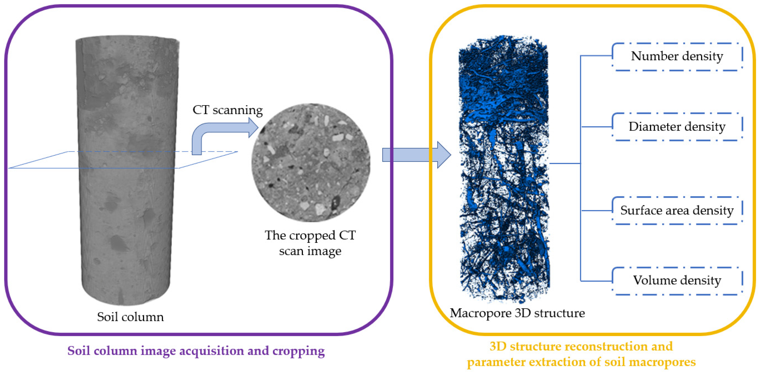
2.5. Industrial CT Scanning and 3D Soil Structure Determination

The 18 soil columns were spirally scanned by using an industrial cone beam CT system with a scanning voltage of 450 kV, current of 10 mA, and a scanning interval of 0.215 mm. Each column yielded 1394 scanning cross-sectional images of 1024 × 1024 pixels. To reduce edge effects of the tube on soil structure, we cropped images within 5 mm of the boundary. Considering the scanning technique and the loose structure of the surface soil, which is easily disturbed, 35 mm of the upper and lower ends of the columns were excluded from the analyses to ensure reliability of the scan results. Thus, the column length of the 0–10 cm and 20–30 cm soil depths was reduced to 35–100 mm and 200–265 mm, respectively (Figure 4). Similar to previous studies, and the limitation of output image accuracy of the CT scanning equipment, we defined the minimum diameter of macropores as 0.3 mm [29,30]. The extracted soil macropore parameters were integrated with the data in a minimum unit layer of 10 mm to obtain the parameters of macropore number, diameter, surface area, and volume. To analyze Ks data of each layer, the macropore density parameters corresponding to each layer of soil were obtained by taking 100, 200, and 265 mm as the boundary points. In addition, considering that soil samples were obtained from both sides of the soil column, the macropore parameters of each soil column were divided into two parts, which were based on the volume of the semi-cylinder; thus, we obtained 108 groups of macropore parameters corresponding to the Ks and soil physicochemical property data sampled nearby.

2.6. Evaluation of PTF Models

The geometric mean error ratio (GMER), root mean square error (RMSE), and AIC (Akaike’s information criterion) were used to evaluate the accuracy of the models:

$$GMER=Exp\left[\frac{1}{n}\sum _{i=1}^{n}ln\left(\frac{{Ks}_{pi}}{{Ks}_{mi}}\right)\right]$$

(5)

$$RMSE=\sqrt{\frac{1}{n}\sum _{i=1}^n{\left({Ks}_{pi}-{Ks}_{mi}\right)}^2}$$

(6)

$$AIC=2k+nln\left[\sum _{i=1}^n{\left({Ks}_{pi}-{Ks}_{mi}\right)}^2\right]$$

(7)

where $n$ is the number of samples, ${Ks}_{pi}$ is the predicted Ks of the $i$th sample, ${Ks}_{mi}$ is the measured Ks of the $i$th sample, and $k$ is the number of PTF models. In addition, GMER represents the average deviation between predicted and measured values. GMER = 1 means values are completely consistent; GMER > 1 means that the predicted value of the model is higher than the measured value; GMER < 1 means that the prediction of the model is lower. RMSE indicates the prediction accuracy; the smaller the RMSE, the better the prediction accuracy. The AIC index can weigh the complexity of the model and the goodness of the model fitting data; a small AIC indicates a better model fit. Therefore, the smaller the RMSE and AIC, the better the prediction of the model.

2.7. Data Processing

The CT images were extracted by the label analysis function in Avizo 9.0.1 to quantify the macropore parameters. Basic data entry and processing of soil physicochemical properties and Ks were performed in Excel 2020. Analysis of variance, Pearson correlation, and regression were calculated by using SPSS 22.0, and the graphics were completed in Excel 2020 and Origin 2022.

3. Results

3.1. Ks in Different Forest Soils

The distribution of Ks in 0–10 cm, 10–20 cm, and 20–30 cm soil depth for the six forest types is shown in Figure 5. The different color bars in each plot show that Ks tends to decrease with increasing soil depth. However, for pure Pinus tabulaeformis Carrière (Plot 1, coniferous forest), the Ks was almost constant, with a small increase with soil depth. The Ks of Plot 1 was small, while mixed forests generally showed high Ks. Overall, the Ks was related as coniferous forest < broad-leaved forest < mixed forest. Notably, the Ks of Pinus tabulaeformis Carrière–Castanea mollissima Blume–Ulmus pumila L. mixed forest (Plot 6) showed significant differences (p < 0.05) among the three soil layers. The Ks of the 20–30 cm soil layer (1.83 ± 0.32 mm·min⁻¹) was 64.2% lower than that of the 10–20 cm soil layer (5.10 ± 1.15 mm·min⁻¹), and 71.7% lower than that of the 0–10 cm soil layer (6.46 ± 1.17 mm·min⁻¹). Meanwhile, the pure Castanea mollissima Blume (Plot 2) and Juglans regia L. (Plot 4) forests showed significant differences (p < 0.05) between the 0–20 cm and 20–30 cm layers. In addition, the decrease in Ks from the top to bottom of each soil layer was 35.3%, 35.8%, 45.9%, 25.7%, and −23.0% for Pinus tabulaeformis Carrière–Castanea mollissima Blume mixed forest (Plot 5), Ulmus pumila L. pure forest (Plot 3), Castanea mollissima Blume pure forest (Plot 2), Juglans regia L. pure forest (Plot 4), and Pinus tabulaeformis Carrière pure forest (Plot 1), respectively. Overall, the variation range of Ks of mixed forests with soil depth was larger than that of pure forests.

In addition, in Figure 5, same-color bars show the average Ks at 0–10, 10–20, and 20–30 cm soil depth, respectively. Among them, the greatest variation in Ks was observed in the 0–10 cm soil layer, by up to 196%, and there was a significant difference in Ks between the mixed and pure forests (p < 0.05). With the increase of soil depth, the variation of Ks among the stands decreased, and the overall variation of Ks in the 10–20 and 20–30 cm soil layers was 117% and 106%, respectively. It is worth noting that, in the 0–20 cm layer, Ks in each plot showed more significant differences than that in the 20–30 cm layer (p < 0.05).

3.2. Relationships between Soil Physicochemical Properties of Different Forest Types on Ks

Table 2. Two-way repeated ANOVA test between soil physicochemical properties of different forest type.

Parameter	Ks	Bulk Density	Water Content	Sand	Silt	Organic Matter	Total Nitrogen	Total Phosphorus	Total Potassium
Forest type	8.438 **	6.943 **	13.165 **	88.626 **	88.604 **	22.647 **	13.122 **	2.523 *	20.654 **
Soil depth	8.048 **	8.120 *	3.282 *	0.871	0.875	23.301 **	21.612 **	4.158 *	26.354 **
Forest type × Soil depth	7.708 **	5.183 **	9.727 **	112.737 **	112.751 **	350.879 **	29.434 **	17.167 **	76.793 **

Note: * significant relationship at 0.05 level, ** significant relationship at 0.01 level.

shows the two-way repeated ANOVA test for soil physicochemical properties of the six forest types. As shown in Table 2, forest type had a highly significant relationship (p < 0.01) with Ks, bulk density, water content, sand, silt, organic matter, total nitrogen, and total potassium content, and a significant relationship (p < 0.05) with total phosphorus content. Soil depth had a highly significant relationship with Ks, bulk density, organic matter, total nitrogen, and total potassium content (p < 0.01), and a significant relationship with water content and total phosphorus (p < 0.05), but had no significant relationship with sand and silt. The relationship between stand type and soil depth was highly significant for all parameters (p < 0.01) This indicates that both stand type and soil depth have certain relationship with soil physicochemical properties, thereby affecting Ks.

To further explore the effects of soil on Ks, the above eight physicochemical properties were selected as variables for Pearson correlation analysis (Figure 6). The correlation order of each variable was bulk density > organic matter > total nitrogen > total potassium > water content > total phosphorus > sand and silt. Bulk density and sand were negatively correlated with Ks. The remaining variables were positively correlated with Ks. The correlations between bulk density, organic matter, total nitrogen, total potassium, and Ks were the strongest (p < 0.001), with correlation coefficients of −0.868, 0.580, 0.378, and 0.346, respectively. In addition, the remaining soil physicochemical properties were correlated with each other to different degrees, indicating that the soil physicochemical properties interact with each other. Soil bulk density was significantly negatively correlated with organic matter, total nitrogen, and total potassium (p < 0.001). Organic matter was significantly positively correlated with total nitrogen and total potassium (p < 0.001).

3.3. Characteristics of Soil Macropore Structure and Effect on Ks

The soil macropore structure varied for different forest types. It can be seen from Figure 7 that the number density, length density, surface area density, and volume density of macropores show a “wave” of decreasing trend as the soil depth increases, and all the indicators showed mixed forests > pure forests. In addition, the difference in macropore structure characteristics of different stands was larger in the surface soil, but the difference gradually decreased with increasing soil depth, indicating that the deeper the soil, the less the variation.

It can be seen from Figure 7a that the overall relation for number density was as follows: plot 4 < plot 3 < plot 1 < plot 2 < plot 5 < plot 6, i.e., the overall number density of pure forests was lower than that of mixed forests. Among them, the number density of plot 1 and plot 4 increased sharply in the 200 mm soil layer. However, when analyzed in conjunction with Figure 7b–d, the macropore length density, surface area density, and volume density did not display a significant change. Plot 1 and Plot 4, in the 200 mm soil layer, were dominated by small-diameter macropores, and the number increased significantly. The reason may be due to the increase of microbial and animal activities in this soil layer and the increase in the number of fine roots of plants. Additionally, in the 200 mm soil layer, Figure 7b shows that there was a sudden increase in the macropore length density of Plots 3 and 5. However, combined with Figure 7a,c,d, the number density, surface area density, and volume density did not show a major change. This indicates that elongated pores may be present in this layer in Plots 3 and 5. As Figure 7c–d shows, there is a general increase in macropore surface area density and volume density with increasing soil depth for all forest types.

Further correlation analysis of macropore structure can be seen from Figure 8. Ks showed a highly significant positive correlation with macropore length density, volume density, surface area density, and number density (p < 0.001). Among them, volume density had the strongest correlation with Ks (R_VKs = 0.676), followed by number density, and then surface area density. The lowest correlation was length density (R_LKs = 0.533). In addition, the length density, volume density, surface area density, and number density showed highly significant positive correlations with each other (p < 0.001). With the exceptions of length density and surface area density (R_LS = 0.673), and length density and number density (R_LN = 0.634), the correlation between macropores structures was stronger than correlation with Ks (R_LN < R_LS < 0.676 < 0.720 < 0.758 < 0.857 < 0.900).

3.4. Construction of PTFs Model for Ks

The above analyses showed that differences in soil physicochemical properties and soil macropore structure characteristics affect Ks. Previous similar studies [31] have used a correlation R > 0.1 and significance p < 0.2 as criteria for predicting Ks. In addition, considering that soil water content is affected by changes in time and meteorological factors, its variable property is not suitable as an index for the construction of PTF. Thus, eleven factors of 72 groups soil physicochemical properties (bulk weight, sand, silt, organic matter, total nitrogen, total phosphorus, and total potassium) and macropore characteristics (length density, bulk density, surface area density, and number density) were used for stepwise multiple regression of Ks. Using this procedure, length density, bulk density, and water content were used to construct PTF1 (

Table 3. Multiple regression of Ks.

PTFs	Regression	R2	Significance Level (p)
PTF1	$K_s=20.63-12.168BD+7.677\rho \left(D\right)+0.373P$	0.887	<0.01
PTF2	$K_s=23.992-13.845BD+0.342P+0.224SOM$	0.844	<0.01
PTF3	$K_s=1.231-5.078\rho \left(N\right)+17.799\rho \left(D\right)+45.342\rho \left(S\right)+1.746\rho \left(V\right)$	0.493	<0.01

$BD$ represents bulk density (g·cm⁻³), $SOM$ organic matter content (%), $P$ total phosphorus (mg·kg⁻¹), $\rho \left(N\right), \rho \left(D\right), \rho \left(S\right), \mathrm{a}\mathrm{n}\mathrm{d} \rho \left(V\right)$ number density (number·mm⁻³), length density (mm·mm⁻³), surface area density (mm⁻²·mm⁻³), and volume density (mm⁻³·mm⁻³) of macropores, respectively.

). Increasing the number of factors, without the soil macropore parameters, slightly increased the R² (PTF2 in Table 3). To investigate whether Ks can be deduced only through the soil macropores parameters, PTF3 was regressed only with length density, volume density, surface area density, and number density of macropores (Table 3). However, this resulted in a much lower R² (Table 3).

Furthermore, we used another 36 groups of measured data to verify the newly constructed PTFs. As can be seen from Figure 9, the regression coefficients of PTF1 and PTF2 were much higher than those of PTF3. Regression points for PTF1 and PTF2 were well distributed on each side of the 1:1 line (Figure 9a,b). GMER for PTF1 and PTF2 were both less than 1, while the GMER for PTF3 was greater than 1, indicating that the predicted PTF1 and PTF2 were slightly low and the PTF3 slightly high. The RMSE and AIC values of PTF1 and PTF2 were close to each other, and both were less than those of PTF3. Meanwhile, the AIC values of PTF1 and PTF2 were −123.964 and −125.647, respectively, which were much lower than those of PTF3 (143.309), indicating that PTF1 and PTF2 were better at estimating Ks. Accordingly, the PTF1 and PTF2 estimates were similar, and the PTF1 estimate was slightly better than that of PTF2.

4. Discussion

4.1. Characteristics of Ks and Its Influencing Factors

The results showed that the Ks of each plot was low for Pinus tabulaeformis Carrière. Previous studies have shown that the Ks of broad-leaved forest is higher than that of coniferous forests [32]. This is consistent with our results. The smallest soil macropore surface area density and volume density were found for Pinus tabulaeformis Carrière forest. The number density and length density were also small for this type of forest, showing that Pinus tabulaeformis Carrière soil is more compact, as compared to other forest types. This explains the low Ks of Pinus tabulaeformis Carrière forest, to some extent. In addition, the overall Ks of mixed forests was higher than that of pure forests. Combined with soil macropore parameters, the number, length, surface area, and volume of macropores in mixed forest were higher than those in pure forests. With the increase of macropores, water moves more easily, and Ks increases accordingly. With the increase of soil depth, the difference of Ks among different forest types showed a decreasing trend. This can be explained by a higher activity of animals and plants in the shallower soil layer, which promotes the development of less compact soil in the upper layer [31]. In contrast, deeper soils are less disturbed by external factors, thus the difference in Ks becomes smaller. This is also supported by the fact that macropore structures decrease with increasing soil depth. The results of this study indicated that both stand type and soil depth affect soil physicochemical properties, which in turn affect the Ks. Different stand types have different plant root configurations, which can change the pore structure of the soil by coiling and twisting in the soil layer, thus changing the permeability of the soil. In addition, both the growth expansion and decomposition processes of coarse roots are likely promote the formation of soil macropores [33,34] and increase Ks [6,35], while fine roots may reduce the macropore channels that can infiltrate water by filling the soil macropore space, thus reducing Ks [35]. Secondly, the distribution of plants, animals, and microorganisms under different stand structures is different, and the metabolism and decomposition products of their life activities are different, which in turn leads to different nutrients released into the soil to change soil fertility to different degrees, thus causing differences in soil chemical properties. Third, the soil physicochemical properties will change with increasing soil depth, which is related to the subsurface root distribution in the vertical direction and the regional differences of soil animal and microbial life.

In the correlation analysis between Ks and various physicochemical properties, it was found that the correlations between Ks and soil bulk density, water content, organic matter and total nitrogen content were highly significant, while that between Ks and total potassium was significant. Notably, although water content is a variable affected by time and meteorological factors (such as rainfall), soil porosity differences of different forestlands lead to differences in water holding capacity, thus affecting the index of water content. Therefore, the results of this study showed that water content was correlated with Ks, but could not prove that there was a direct relationship between the two. The correlations between Ks and sand, silt, and total phosphorus were not significant. This is consistent with most previous research conclusions [33,36], and at the same time is in accordance with previous studies in this region [37]. The correlation among the remaining physicochemical indicators varied, suggesting that the effect of soil physicochemical properties on Ks may arise through interaction with other indicators, and that this "coordinated" effect may be either a positive or a negative effect [38]. Organic matter content was significantly positively correlated with the Ks, which is in accordance with previous research [39]. Soil organic matter is important in the cohesive cementation process of soil aggregates, and has a positive role in the formation and stabilization of aggregates; soil aggregates are the basis of soil structure formation, and soil stability has a direct impact on soil infiltration. Therefore, soil organic matter can affect soil Ks by changing soil structure. Studies have shown that soil porosity will increase with the increase of organic matter content [40,41], as the increase of soil organic matter will aggravate the metabolic activities of soil animals, plants, and microorganisms; therefore, increasing soil porosity could lead to an increase in Ks. Moreover, some studies have pointed out that the higher the soil organic carbon content, the better the soil structure development, and the better the structural stability [3]. In addition, the number density, length density, and surface area density results are consistent with the conclusion of previous studies that the water infiltration capacity can be determined by characterizing the spatial parameters of soil macropores (e.g., macropore length, macropore surface area, macropore volume, etc.) [42,43,44]. Furthermore, volume density of macropores was significantly positively correlated with Ks. This indicates that each index will not only directly affect Ks, but also change Ks through the interaction between the macropore spatial structure indexes.

4.2. Applicability of PTFs to Predict Ks

Evaluation of PTFs with different input parameters showed that the predictions of PTF1 and PTF2 were significantly better than those of PTF3. PTF1 included soil bulk density, total phosphorus, and soil macropore length density. Thus, CT scanning is necessary and greatly increases the experimental cost. On the other hand, PTF2 only needs to measure a limited number of physicochemical parameters. Thus, PTF2 may be more practical. In contrast, PTF3, using only soil macropore parameters, did not provide good results. The reason for this may be that the macropore parameters selected in this study do not directly indicate water transport. The four parameters are oriented towards individual pore conditions but ignore the connectivity of macropores. Not all soil macropores contribute to water infiltration, and soil structures with high connectivity are more preferential in transporting water and solute downward [12]. In addition, the degree of closure of macropores and the air condition in macropores could affect water migration [18,45]. It is worth noting that the original intention of PTF3 was regarding the fact that CT technology is being used in more and more soil structure studies, and Ks is often also an indicator of concern to scholars. However, for these researchers, if only the macropore parameters are used to calculate Ks, the time and cost of measurement can be greatly reduced. For other scholars who do not conduct CT research, it is not necessary to consider this PTF.

Measured Ks was predicted by using previously published PTFs models (Cosby [46], Campbell [47], Vereecken [48], Julià [49]). The specific expressions are shown in

Table 4. Empirical PTF models used in this study.

PTFs	Empirical PTF Expressions
Cosby	$K_S=60.96\times {10}^{\left(-0.6+0.0126C_3-0.0064C_1\right)}$
Campbell	$K_s=3.456\times {10}^2\times {\left(\frac{1.3}{BD}\right)}^{1.3b}\times e^a$ $a=-2.5\times {10}^{-2}-6.88\times {10}^{-2}{c}_1-3.63\times {10}^{-2}{c}_2$ $b=\sqrt{e^a}+0.2\times \sqrt{e^{\left(0.133c_2+0.477c_1-ln2e^a\right)}}$
Vereecken	$K_S=e^{\left(20.62-0.96log\left(C_1\right)-0.66log\left(C_3\right)-0.46log\left(SOM\right)-8.43BD\right)}$
Julià	$K_S=2.4\times \left(-4.994+0.56728C_3-0.131C_1-0.0127SOM\right)$

$C_1, C_2$, and $C_3$ represent the content of clay, silt, and sand (%), respectively. BD represents soil bulk density (g·cm⁻³) and $SOM$ represents organic matter content (g·kg⁻¹).

, and measured and predicted Ks values are compared (Figure 10). The GMER values of the four groups are greater than one, and as well greater than the GMER in our study. It can also be seen from Figure 10 that the points are mostly distributed to the left of the 45° line, with Cosby, Vereecken, and Julià deviating to a greater extent than Campbell. The RMSE and AIC values of all four groups were also much higher than those of our presented PTFs. Especially, the Vereecken model overestimated the Ks. In other words, the prediction accuracy of the new PTFs is much better for the study area. The reason for the high prediction accuracy may be the absence of clay in our experimental area. It is worth noting that, although the prediction effect of PTF3 in this study is far inferior to that of PTF1 and PTF2, it is still better than previous models. In the future, it may be possible to consider the introduction of other spatial structure parameters, such as soil macropore connectivity, gravel properties, and roots, into the construction of soil PTFs to improve prediction accuracy.

5. Conclusions

Simplified soil Ks estimations can be performed using soil physicochemical properties and soil macropore parameters. We proposed PTFs for Ks prediction in typical forestland in the rocky mountain area of Northern China. The main conclusions are as follows:

(1)

Observed Ks of typical forest soil in rocky mountain areas of Northern China showed an overall decrease with depth, and the relation coniferous < broadleaf < mixed forest. The variation in mixed forests was greater than that of pure forests, especially in the surface layer (0–10 cm) of soil, where the Ks of mixed forests was significantly greater than that of pure forests.

(2)

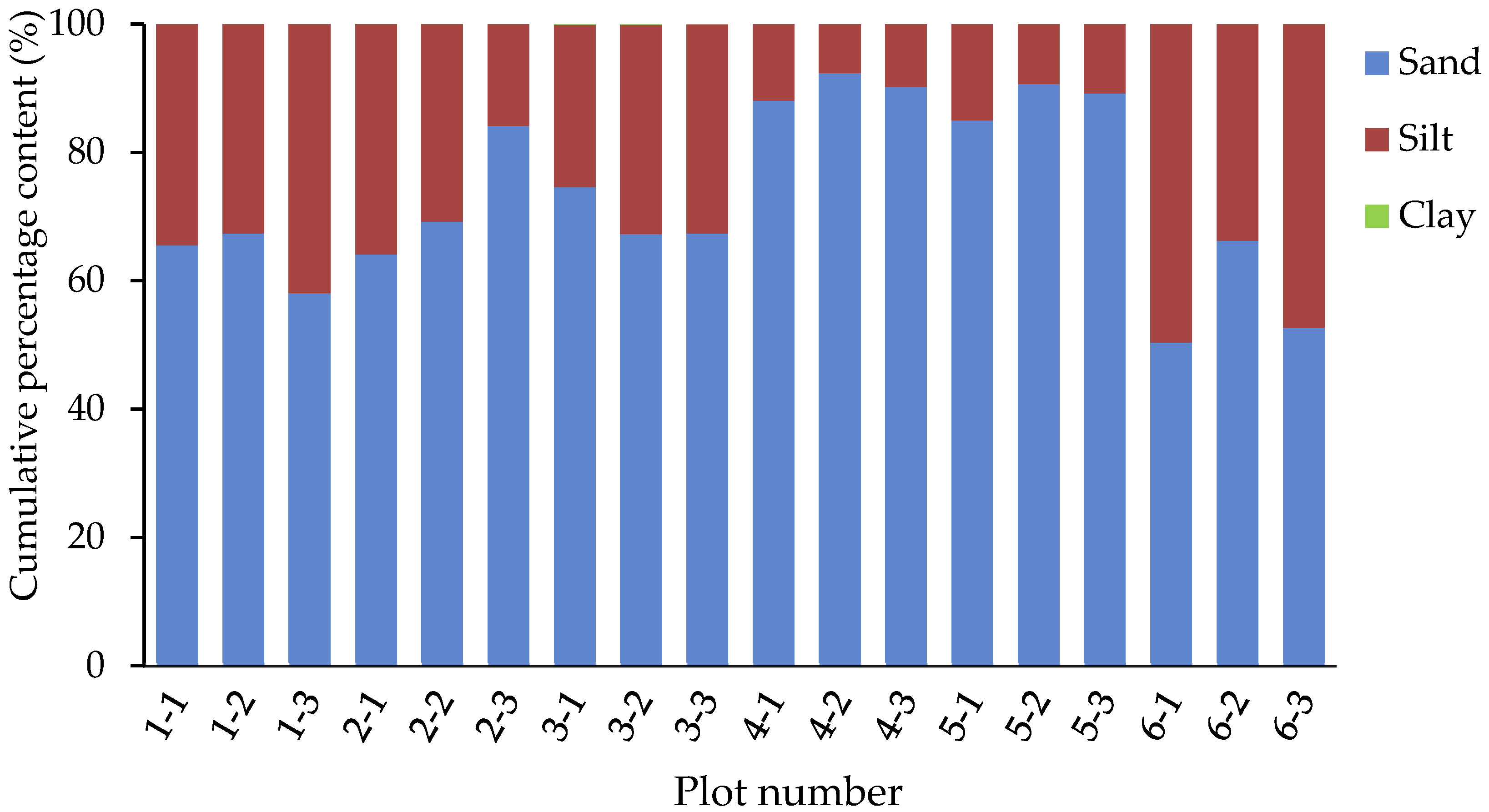
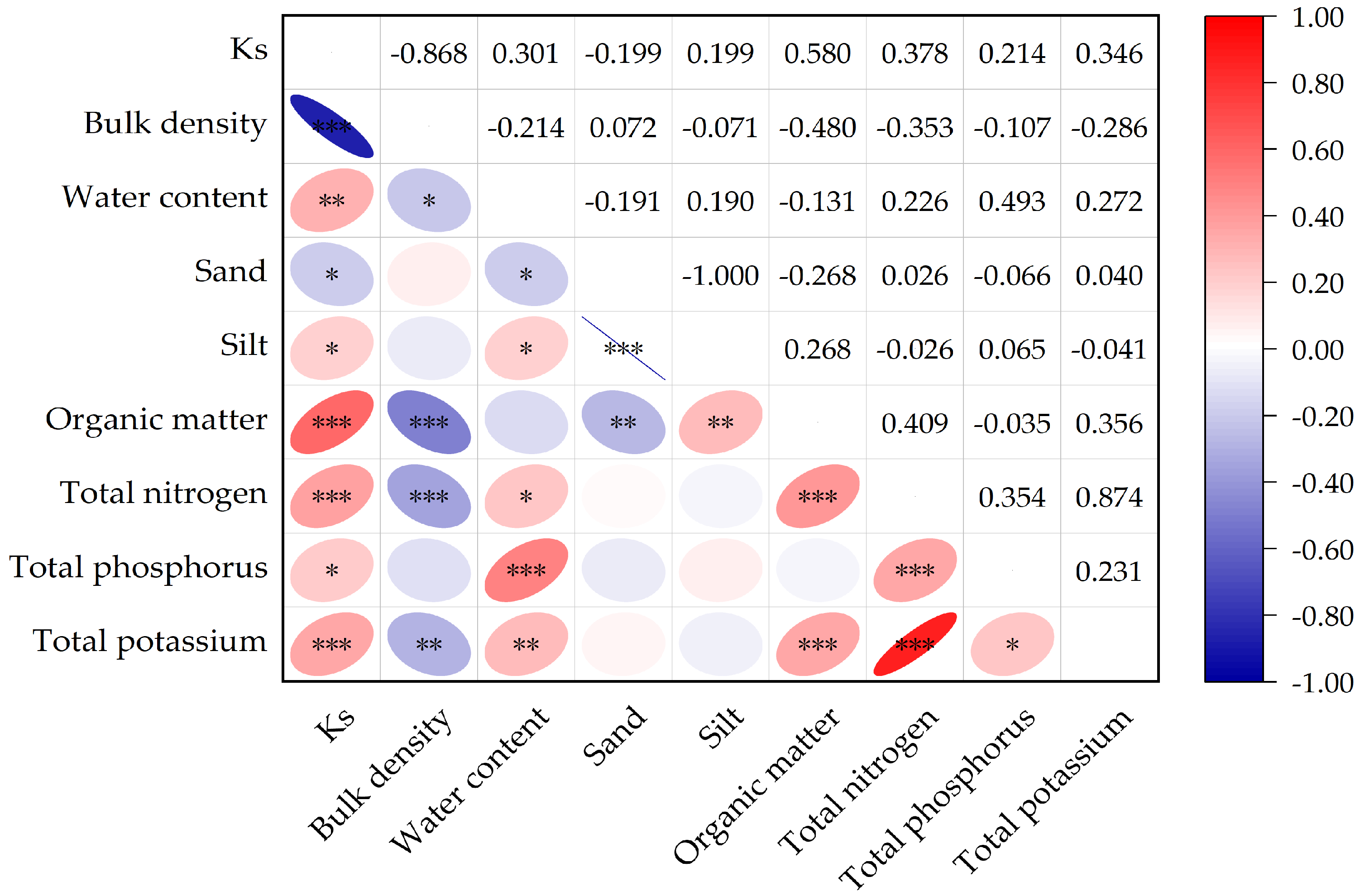
For soil physicochemical properties, organic matter (p < 0.001), total nitrogen (p < 0.001), total potassium (p < 0.001), water content (p < 0.01), silt (p < 0.05), and total phosphorus (p < 0.05) were significantly positively correlated with Ks, while bulk density (p < 0.001) and sand (p < 0.05) were significantly negatively correlated with Ks. Moreover, both forest type and soil depth had certain effects on soil physicochemical properties, thereby affecting soil Ks.

(3)

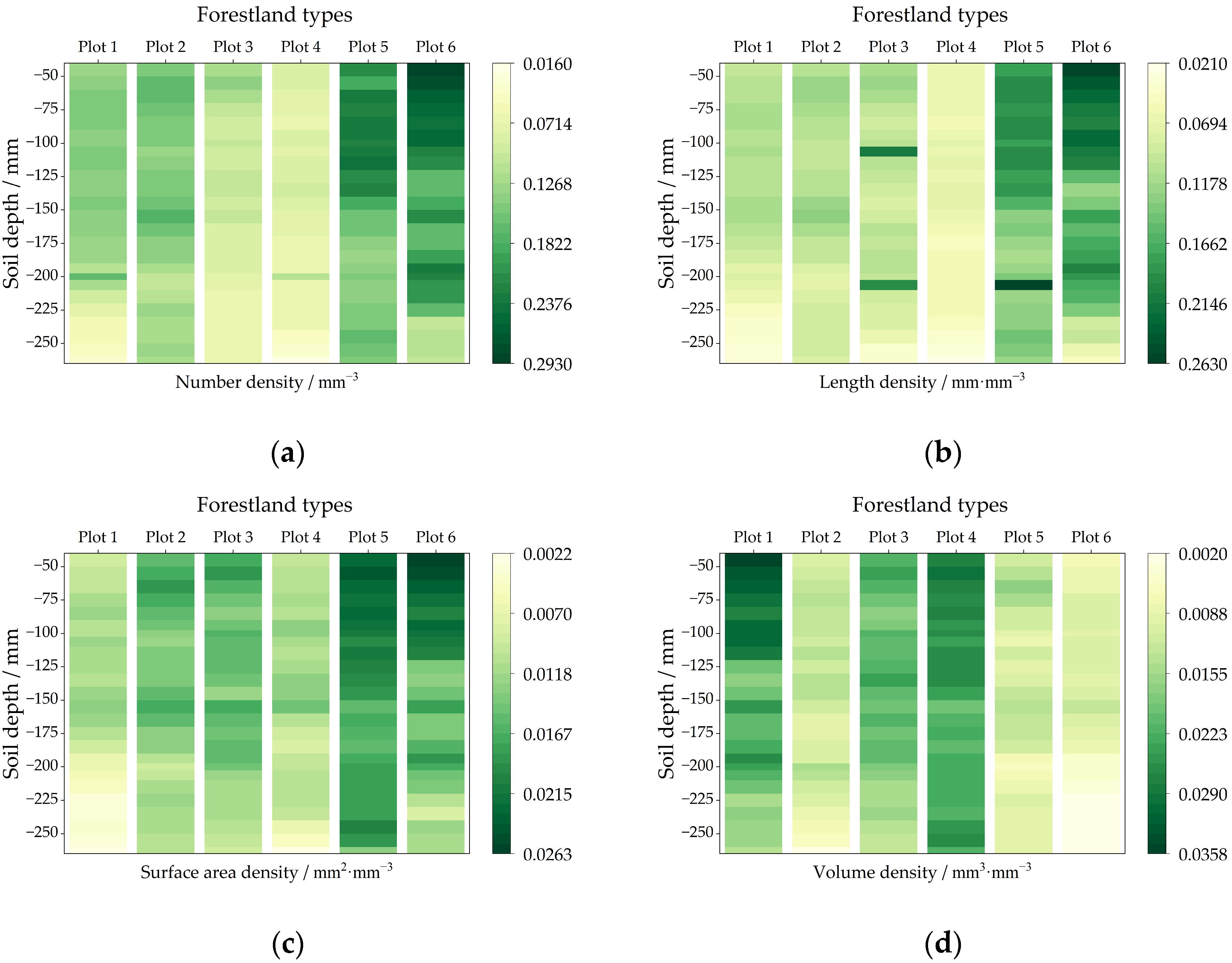
The number density, length density, surface area density, and volume density of soil macropore structure showed a decreasing trend with increasing soil depth, and they were all significantly positively correlated with Ks (p < 0.001). The parameters of macropore spatial structure were significantly positively inter-correlated (p < 0.001).

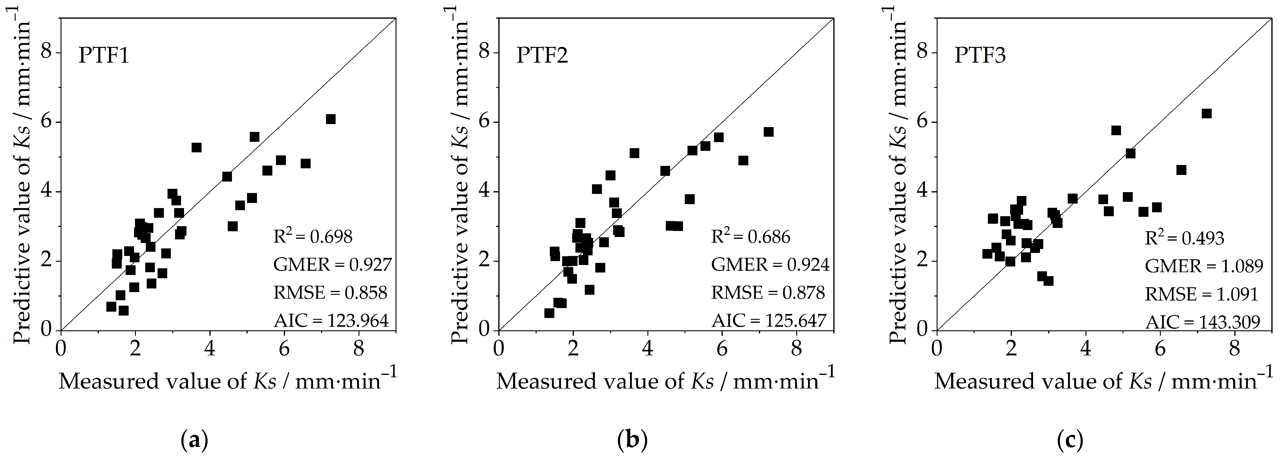
(4)

The PTF2 (GMER = 0.924, RMSE = 0.878, AIC = 125.647) constructed by soil bulk density, organic matter, and total phosphorus was the best and most applicable among the three investigated PTFs. The prediction results of the three new PTFs were better than previously presented PTF models (Cosby, Campbell, Vereecken, and Julià).

(5)

Prediction of Ks using only parameters of macropore spatial structure did not provide satisfactory results. However, it may provide new ideas for future improved Ks PTFs. In the future, other soil structural parameters obtained by CT scanning can be considered to improve the accuracy of the prediction model.

References

1. Hou, G.R.; Bi, H.X.; Wei, X.; Zhou, Q.Z.; Kong, L.X.; Wang, J.S.; Jia, J.B. Water conservation function of litters and soil in three kinds of woodlands in gully region of Loess Plateau. J. Soil Water Conser. 2018, 32, 357–363+371. [Google Scholar] [CrossRef]
2. Parchami-Araghi, F.; Mirlatifi, S.M.; Dashtaki, S.G.; Mahdian, M.H. Point estimation of soil water infiltration process using Artificial Neural Networks for some calcareous soils. J. Hydrol. 2013, 481, 35–47. [Google Scholar] [CrossRef]
3. Ghorbani-Dashtaki, S.; Homaee, M.; Loiskandl, W. Towards using pedotransfer functions for estimating infiltration parameters. Hydrol. Sci. J. 2016, 61, 1477–1488. [Google Scholar] [CrossRef] [Green Version]
4. Xu, C.C.; Xu, X.L.; Liu, M.X.; Liu, W.; Yang, J.; Luo, W.; Zhang, R.F.; Kiely, G. Enhancing pedotransfer functions (PTFs) using soil spectral reflectance data for estimating saturated hydraulic conductivity in southwestern China. Catena 2017, 158, 350–356. [Google Scholar] [CrossRef]
5. Klute, A.; Dirksen, C. Hydraulic conductivity and diffusivity: Laboratory methods. In Methods of Soil Analysis: Part 1—Physical and Mineralogical Methods; American Society of Agronomy—Soil Science Society of America: Madison, WI, USA, 1986; Volume 5, pp. 687–734. [Google Scholar] [CrossRef]
6. Zhu, P.Z.; Zhang, G.H.; Zhang, B.J. Soil saturated hydraulic conductivity of typical revegetated plants on steep gully slopes of Chinese Loess Plateau. Geoderma 2022, 412, 115717. [Google Scholar] [CrossRef]
7. Germann, P.F.; Beven, K. Kinematic wave approximation to infiltration into soils with sorbing macropores. Water Resour. Res. 1985, 21, 990–996. [Google Scholar] [CrossRef]
8. Watson, K.W.; Luxmoore, R.J. Estimating macroporosity in a forest watershed by use of a tension infiltrometer. Soil Sci. Soc. Am. J. 1986, 50, 578–582. [Google Scholar] [CrossRef]
9. Hayashi, Y.; Ken’ichirou, K.; Mizuyama, T. Changes in pore size distribution and hydraulic properties of forest soil resulting from structural development. J. Hydrol. 2006, 331, 85–102. [Google Scholar] [CrossRef]
10. Soto-Gómez, D.; Pérez-Rodríguez, P.; Vázquez-Juiz, L.; Lopez-Periago, J.E.; Paradeloa, M. Linking pore network characteristics extracted from CT images to the transport of solute and colloid tracers in soils under different tillage managements. Soil Tillage Res. 2018, 177, 145–154. [Google Scholar] [CrossRef]
11. Yang, Y.H.; Wu, J.C.; Zhao, S.W.; Han, Q.Y.; Pan, X.Y.; He, F.; Chen, C. Assessment of the responses of soil pore properties to combined soil structure amendments using X-ray computed tomography. Sci. Rep. 2018, 8, 695. [Google Scholar] [CrossRef] [Green Version]
12. Katuwal, S.; Norgaard, T.; Moldrup, P.; Lamandé, M.; Wildenschild, D.; de Jonge, L.W. Linking air and water transport in intact soils to macropore characteristics inferred from X-ray computed tomography. Geoderma 2015, 237–238, 9–20. [Google Scholar] [CrossRef]
13. Larsbo, M.; Koestel, J.; Jarvis, N. Relations between macropore network characteristics and the degree of preferential solute transport. Hydrol. Earth Syst. Sci. 2014, 18, 5255–5269. [Google Scholar] [CrossRef] [Green Version]
14. Li, J.Z.; Pei, T.F.; Li, X.Y.; Niu, L.H. Models of soil saturated infiltration coefficient and effective porosity in forest catchment. Chin. J. Appl. Ecol. 1998, 6, 597–602. Available online: http://www.cjae.net/CN/abstract/abstract4925.shtml (accessed on 18 December 1998).
15. Shi, Z.J.; Wang, Y.H.; Xu, L.H.; Xiong, W.; Yu, P.T.; Guo, H.; Xu, D.P. The influence of rock fragments on the characteristics of macropore and water effluent of forest soils in the Liupan Mountains, Northwest China. Acta Ecol. Sin. 2008, 10, 4929–4939. [Google Scholar] [CrossRef]
16. Wang, Z.W.; Shao, M.A.; Huang, L.M.; Pei, Y.W.; Li, R.L. Distribution and Influencing Factors of Soil Saturated Hydraulic Conductivity Under Different Land Use Patterns in Eastern Qinghai Province. J. Soil Water Conser. 2021, 35, 150–155. [Google Scholar] [CrossRef]
17. Zheng, H.; Han, L.; Shojaaddini, A. Predicting saturated hydraulic conductivity by pedo-transfer function and spatial methods in calcareous soils. J. Appl. Geophys. 2021, 191, 104367. [Google Scholar] [CrossRef]
18. Koestel, J.K. Links between soil properties and steady-state solute transport through cultivated topsoil at the field scale. Water Resour. Res. 2013, 49, 790–807. [Google Scholar] [CrossRef] [Green Version]
19. Baver, L.D. Soil permeability in relation to non-capillary porosity. Soil Sci. Soc. Am. J. 1939, 3, 52–56. [Google Scholar] [CrossRef] [Green Version]
20. Liu, S.Z.; Wang, Y.Q.; An, Z.S.; Sun, H.; Zhang, P.P.; Zhao, Y.L.; Zhou, Z.X.; Xu, L.; Zhou, J.X.; Qi, L.J. Watershed spatial heterogeneity of soil saturated hydraulic conductivity as affected by landscape unit in the critical zone. Catena 2021, 203, e105322. [Google Scholar] [CrossRef]
21. Becker, R.; Gebremichael, M.; Märker, M. Impact of soil surface and subsurface properties on soil saturated hydraulic conductivity in the semi-arid Walnut Gulch Experimental Watershed, Arizona, USA. Geoderma 2018, 322, 112–120. [Google Scholar] [CrossRef]
22. Fang, L.J.; Gao, R.Z.; Liu, T.X.; Zhang, A.L.; Wang, X.X. Construction and evaluation of pedo-transfer functions in the Balager River Basin. Arid Zone Res. 2020, 37, 1156–1165. [Google Scholar] [CrossRef]
23. Schaap, M.G.; Leij, F.J.; van Genuchten, M.T. Neural network analysis for hierarchical prediction of soil hydraulic properties. Soil Sci. Soc. Am. J. 1998, 62, 847–855. [Google Scholar] [CrossRef]
24. Minasny, B.; McBratney, A.B. Evaluation and development of hydraulic conductivity pedotransfer functions for Australian soil. Soil Res. 2000, 38, 905–926. [Google Scholar] [CrossRef]
25. Minasny, B.; Mcbratney, A.B. The neuro-m method for fitting neural network parametric pedotransfer functions. Soil Sci. Soc. Am. J. 2002, 66, 352–361. [Google Scholar] [CrossRef] [Green Version]
26. Yang, S.E.; Huang, Y.F. Prediction of soil hydraulic characteristic parameters based on support vector machine. Trans. Chin. Soc. Agric. Eng. 2007, 7, 42–47. [Google Scholar] [CrossRef]
27. Meng, C.; Niu, J.Z.; Li, X.; Luo, Z.T.; Du, X.Q.; Du, J.; Lin, X.N. Quantifying soil macropore networks in different forest communities using industrial computed tomography in a mountainous area of North China. J. Soils Sediments 2017, 17, 2357–2370. [Google Scholar] [CrossRef]
28. Nachtergaele, F.; Velthuizen, H.V.; Verelst, L.; Batjes, N.H.; Dijkshoorn, K.; van Engelen, V.W.P.; Fischer, G.; Jones, A.; Montanarella, L.; Petri, M.; et al. The harmonized world soil database. In Proceedings of the 19th World Congress of Soil Science, Soil Solutions for a Changing World, Brisbane, Australia, 1–6 August 2010; pp. 34–37. [Google Scholar]
29. Wu, H.S.; Chen, X.M.; Chen, C. Study on Macropore in Main Paddy Soils in Tai-Lake Region with CT. J. Soil Water Conser. 2007, 02, 175–178. [Google Scholar] [CrossRef]
30. Meng, C.; Niu, J.Z.; Yin, Z.C.; Luo, Z.T.; Lin, X.N.; Jia, J.W. Characteristics of rock fragments in different forest stony soil and its relationship with macropore characteristics in mountain area, northern China. J. Mt. Sci. 2018, 15, 519–531. [Google Scholar] [CrossRef]
31. Luo, Z.T. Features of Preferential Flow and Its Influence Factors in Typical Forests Root Zone in Rocky Mountain Area of Northern China; Beijing Forestry University: Beijing, China, 2020; 103p. [Google Scholar] [CrossRef]
32. Zhang, Z.F.; Zhang, X.Z. Effects of vegetation restoration on soil physical parameters on the Loess Plateau: A meta-analysis based on published data. Prog. Geogr. 2021, 40, 1012–1025. [Google Scholar] [CrossRef]
33. Hao, H.X.; Wei, Y.J.; Cao, D.N.; Guo, Z.L.; Shi, Z.H. Vegetation restoration and fine roots promote soil infiltrability in heavy-textured soils. Soil Tillage Res. 2020, 198, 104542. [Google Scholar] [CrossRef]
34. De Baets, S.; Poesen, J.; Knapen, A.; Barberá, G.G.; Navarro, J. Root characteristics of representative Mediterranean plant speciesand their erosion-reducing potential during concentrated runoff. Plant Soil 2007, 294, 169–183. [Google Scholar] [CrossRef]
35. Lu, J.; Zhang, Q.; Werner, A.D.; Li, Y.; Jiang, S.; Tan, Z. Root-induced changes of soil hydraulic properties–A review. J. Hydrol. 2020, 589, 125203. [Google Scholar] [CrossRef]
36. Godoy, V.A.; Zuquette, L.V.; Gómez-Hernández, J.J. Spatial variability of hydraulic conductivity and solute transport parameters and their spatial correlations to soil properties. Geoderma 2019, 339, 59–69. [Google Scholar] [CrossRef]
37. Gao, P.F.; Ran, Z.L.; Han, Z.; Li, J.W.; Li, L.T.; Wei, C.F. Hydraulic properties and saturated hydraulic conductivity pedo-transfer function of rocky purple soil. Acta Pedol. Sin. 2021, 58, 128–139. [Google Scholar] [CrossRef]
38. Huang, W.X.; Deng, Y.S.; Xie, F.Q.; Yang, G.R.; Jiang, D.H.; Huang, Z.G. Characteristics of soil saturated hydraulic conductivity on different positions and their controlling factors of granite collapsing gullies. Chin. J. Appl. Ecol. 2020, 31, 2431–2440. [Google Scholar] [CrossRef]
39. Liu, M.X.; Wu, D.; Wu, S.P.; Liao, L.J. Characteristic of soil macropores under various types of forest coverage and their influence on saturated hydraulic conductivity in the Three Gorges Reservoir Area. Acta Ecol. Sin. 2016, 36, 3189–3196. [Google Scholar] [CrossRef]
40. Wang, Z.L.; Zhao, Y.G.; Zhao, S.W.; Huang, J.H.; Du, C.; Ying, N.S. Study on soil saturated hydraulic conductivity and its influencing factors in typical grassland of farmland conversion. Acta Agrestia Sin. 2016, 24, 1254–1262. [Google Scholar] [CrossRef]
41. Walkley, A.; Black, I.A. An examination of the Degtjareff method for determining soil organic matter, and a proposed modification of the chromic acid titration method. Soil Sci. 1934, 37, 29–38. [Google Scholar] [CrossRef]
42. Hu, X.; Li, X.Y.; Li, Z.C.; Gao, Z.; Wu, X.C.; Wang, P.; Lyu, Y.L.; Liu, L.Y. Linking 3-D soil macropores and root architecture tonear saturated hydraulic conductivity of typical meadow soil types in the Qinghai Lake Watershed, northeastern Qinghai–TibetPlateau. Catena 2020, 185, 104287. [Google Scholar] [CrossRef]
43. Pierret, A.; Capowiez, Y.; Belzunces, L.; Moran, C. 3D reconstruction and quantification of macropores using X-ray computedtomography and image analysis. Geoderma 2002, 106, 247–271. [Google Scholar] [CrossRef]
44. Luo, L.; Lin, H.; Halleck, P. Quantifying soil structure and preferential flow in intact soil using X-ray computed tomography. Soil Sci. Soc. Am. J. 2008, 72, 1058–1069. [Google Scholar] [CrossRef] [Green Version]
45. Jarvis, N.J.; Moeys, J.; Koestel, J.; Hollis, J.M. Preferential flow in a pedological perspective. In Hydropedology: Synergistic Integration of Soil Science and Hydrology; Henry, L., Ed.; Elsevier: Amsterdam, The Netherlands, 2012; Chapter 3; pp. 75–120. [Google Scholar] [CrossRef]
46. Cosby, B.J.; Hornberger, G.M.; Clapp, R.B.; Ginn, T.R. A statistical exploration of the relationships of soil moisture characteristics to the physical properties of soils. Water Resour. Res. 1984, 20, 682–690. [Google Scholar] [CrossRef] [Green Version]
47. Campbell, G.S.; Shiozawa, S. Prediction of hydraulic properties of soils using particle-size distribution and bulk density data. In Proceedings of the International Workshop on Indirect Methods for Estimating the Hydraulic Properties of Unsaturated Soils; van Genuchten, M.T., Leij, F.J., Lund, L.J., Eds.; University of California: Riverside, CA, USA, 1992; pp. 317–328. [Google Scholar]
48. Vereecken, H.; Maes, J.; Feyen, J. Estimating unsaturated hydraulic conductivity from easily measured soil properties. Soil Sci. 1990, 149, 1–12. [Google Scholar] [CrossRef]
49. Julià, M.F.; Monreal, T.E.; Jimenez, A.S.D.C.; Melendez, E.G. Constructing a saturated hydraulic conductivity map of Spain using pedotransfer functions and spatial prediction. Geoderma 2004, 123, 257–277. [Google Scholar] [CrossRef]
Figure 1. Location of the study area Wuzuolou Forest Station, Miyun District in Beijing.
Forests 14 01097 g001
Figure 2. Percentage of soil textural classes in the soil samples. The first number in the plot number represents the plot, with 1 to 6 representing various plots. The second number represents soil depth, with 1 to 3 representing 0–10 cm, 10–20 cm, and 20–30 cm layers, respectively.
Forests 14 01097 g002
Figure 3. Ks measuring device schematic diagram.
Forests 14 01097 g003
Figure 4. Reconstruction of 3D structure of soil macropores and extraction of characteristic parameters.
Forests 14 01097 g004
Figure 5. Distribution characteristics of Ks of different soil layers for different forest types. Lines in the graphs indicate standard deviation, lowercase letters (a–c) indicate significant differences among soil depth in the same forestland (p < 0.05), and different capital letters (A–C) indicate significant differences among different forestland types at the same soil depth (p < 0.05).
Forests 14 01097 g005
Figure 6. Pearson correlation between Ks and soil physicochemical properties. * represents significance (double tail) at 0.05 level, ** significance (double tail) at 0.01 level, and *** significance (double tail) at 0.001 level.
Forests 14 01097 g006
Figure 7. Distribution of soil macropore structure for different forest types. (ad) show the distribution of soil macropore number density, length density, surface area density, and volume density with soil depth.
Forests 14 01097 g007
Figure 8. Pearson correlation analysis of Ks and macropore characteristics. *** represents significant double tail correlation at the 0.001 level.
Forests 14 01097 g008
Figure 9. Comparison between measured and predicted Ks using regressed PTFs. (ac) show the comparison between measured and predicted Ks of PTF1, PTF2, PTF3, respectively.
Forests 14 01097 g009
Figure 10. Comparison between measured and predicted Ks using published PTF models. (ad), respectively, describe the Ks measured values and predicted values of Cosby, Campbell, Vereecken, and Julià models.
Forests 14 01097 g010