Abstract
Heartwood, sapwood, and bark constitute the main components of the tree stem. The stem is the main component of the tree and plays an important role in supporting the tree and transporting nutrients and water. Therefore, quantifying the profiles of heartwood, sapwood, and bark is fundamental to understanding the different components of the tree stem. A seemingly unrelated mixed-effect model system was developed based on 179 destructively sampled trees for 31 permanent sample plots in Korean larch plantation in Northeast China. The heartwood radius and sapwood width were estimated and calibrated only by the observed bark thickness or by all response variables considering the correlations of submodel random effects. The results indicated that the model system achieved good fitting performance and prediction. In addition, after including one to ten bark thickness points and all response variables of sampling below the 2 m height of the tree, the estimated best linear predictor (EBLUP) for local calibration improved the prediction performance, indicating that the heartwood radius and sapwood width could be effectively calibrated by bark thickness while keeping intact the complete inner structure inside the stem. The results provided important information for forest managers and ecologists when selecting appropriate approaches for quantifying the profiles of heartwood, sapwood, and bark.
1. Introduction
For many tree species, a tree stem generally includes three main components: heartwood, sapwood, and bark. Heartwood is the central core of the stem, which is made up of dead tissues transformed by the inner part of the dead sapwood [1,2]. Heartwood is commonly filled with biochemical extractives (e.g., resins, phenols, and terpenes), which increase its stability and biotic resistance. In the timber industry, the size in terms of volume of the heartwood is an essential factor in determining the value of wood. Sapwood is the outer layer of heartwood and is a critical component that sustains the life of a tree because it is responsible for the conduction of sap and resource storage [3]. Sapwood comprises a variety of cell types, such as external rings to transport water and minerals from roots and parenchyma cells to store photosynthate [4,5]. The proportion of heartwood and sapwood varies among species and also varies due to genetics [6], climatic and environmental conditions [1,7], early radial growth [1], and age. Generally, the radius of heartwood decreases with increasing height from the ground level to the tree tip [5,8]. However, the variation of sapwood width with stem height exhibits various patterns that differ among individual trees [2,4,9]. To quantify the profiles of heartwood and sapwood, previous studies focused on mixed-effect linear models [8,10]. However, obtaining the predictor variables in the models (e.g., diameter over bark, heartwood radius at breast height and sapwood width at breast height) can be challenging and time-consuming and usually relies on destructive samples. Additionally, local calibration in the mixed models was not considered in the prediction. Developing reliable statistical models for heartwood and sapwood profiles has not been explicitly examined in the literature.
Bark is the outermost layer of the stem and protects living cambial from insect attack, fire damage, or disease infection. The thickness of tree bark is an important metric for assessing tree susceptibility to fire in fire ecology. Unlike those for heartwood and sapwood profiles, models for predicting bark thickness along the stem have been frequently constructed. For instance, mixed-effect models were used to predict bark thickness for conifer species [11]. The prediction accuracy improved when additional variables were added to bark thickness models [12,13]. Recently, artificial neural networks [14] and a two-stage method (a method combining stem taper function and bark thickness model) [15] showed better performance in prediction bias and precision of bark thickness.
Although several statistical models for predicting the profiles of heartwood, sapwood, and bark have been examined, each component was often predicted by a separate model [8,10,11,12,13,14,15,16,17,18,19,20,21]. The correlation among the models of the three stem components was not considered. The seemingly unrelated mixed-effect (SUR-mixed) model provides a potential approach to quantifying all stem components simultaneously. The SUR-mixed model is an extension of the SUR model for grouped data, which accounts for the correlation between models and the hierarchical structure of the data [22]. The greatest advantage of SUR-mixed model is that it can calibrate hard-measured response variables by easy-measure response variables using their correlation [23]. This modeling approach has been applied in different aspects of forestry research: constructing tree attributes (i.e., diameter at breast height, crown base height, volume, tree height, and dead branch height) [23], tree biomass [24], and stem diameter [25]. To our understanding, applying the SUR-mixed model for characterizing the profiles of different stem components has not been investigated.
Korean larch (Larix olgensis Henry) as a fast-growing species has been widely planted in the northeast of China due to its tolerance to extremely poor soil conditions and cold weather. According to the 9th National Forest Inventory of China (2014–2018), the plantation area in the northeast accounts for approximately 9.2% of the total plantation area in China, and Korean larch occupies approximately 22.3% of the forested area in the northeastern area [26]. Therefore, Korean larch plantations in China provide essential benefits, including carbon storage, biodiversity, economic timber, and other ecosystem services. Thus, accurately quantifying different portions of wood is important, helps understanding the formation of heartwood and sapwood, and provides useful information about tree structure and evidence in timber production.
The objectives of this study were as follows: (1) to develop an unrelated seemingly mixed-effect model system for quantifying heartwood radius, sapwood width, and bark thickness simultaneously, (2) to evaluate the prediction accuracy of submodels, and (3) to estimate the model prediction accuracy and evaluate model’s calibration of different sampling strategies and to select the optimal sampling strategy for different scenarios. This study proposes a quantitative method for characterizing the profiles of heartwood, sapwood, and bark.
2. Materials and Methods
2.1. Study Area and Data Collection
The data in this study were collected from Korean larch plantations across four forestry agencies, which are located in Heilongjiang Province of Northeast China: Linkou Forestry Bureau, Mengjiagang Forest Farm, Dongjingcheng Forestry Bureau, and Maoershan Forestry Farm. The region has a temperate monsoon climate where extreme minimum temperature is −40.1 °C, maximum temperature is 37.0 °C, the mean annual temperature is 2.7 °C, and the mean annual rainfall is 700 mm. The elevations of these four forestry agencies range from 170 m to 900 m above sea level. The geographic locations in this study are shown in Figure 1.
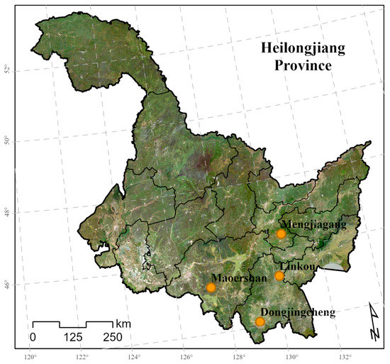
Figure 1.
The locations of the study area in Heilongjiang Province, Northeast China.
A total of 31 sample plots (0.06−0.125 ha in size) in different sites were established in July and August of 2007 to 2008 or 2015 to 2016. The sample plots were distributed in young, medium-age, near-mature, and mature forests. Total tree height (HT), diameter at breast height (DBH, defined as 1.3 m above ground level), crown width in four cardinal directions (CW) and crown length (CL) were measured for all trees in all sample plots. The principle of destructive sampling was to select trees of various sizes that were not dead, crooked, damaged, or diseased with an average diameter at breast height. In each of 19 sample plots established in 2007 and 2008, the trees were divided into five equidistant basal area groups, and one tree was sampled from each group. In each of 12 sample plots established in 2015 and 2016, the trees were divided into five equidistant basal area groups, and one tree was sampled from each group plus the smallest and the largest tree. Overall, a total of 179 trees of 8–53 years were selected.
Before felling the trees, the north and south directions were marked on the trunk. Stem discs approximately 3 to 5 cm thick were obtained at different heights of the log: base, 1 m, 1.3 m, 2 m, and every 1 m along the stem to the top after the total tree height and crown length were measured. Every disc was marked with height and south direction. The stem discs with knots were replaced with their neighboring discs. There were a total of 3356 discs collected in our study. These discs were polished by a belt sander to improve surface visualization of the rings and the color difference between heartwood and sapwood and then scanned. The images of the discs were acquired using image analysis software (WinDENDRO), and the heartwood radius, sapwood width, bark thickness, and stem disc diameter were measured in four directions, as well as the rings for heartwood and sapwood (Figure 2). The radius (R/cm), heartwood radius (HR/cm), sapwood width (SW/cm), and bark thickness (BT/cm) were calculated from the average of the four directions, respectively (Equation (1)). Diameter (D) was twice the radius. The summary of tree and plot statistics is listed in Table 1, and the relationships between heartwood radius, sapwood width, bark thickness, and relative height are shown in Figure 3.
where Y is radius, heartwood radius, sapwood width, and bark thickness.
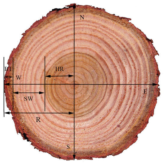
Figure 2.
Measurement of radius (R), heartwood radius (HR), sapwood width (SW), and bark thickness (BT) of Korean larch discs (S—south, W—west, N—north, E—east).

Table 1.
Summary statistics of plot and tree variables of sample trees. Dg—quadratic mean diameter, Hdom—average dominant height, N—density of trees, SI—site index (dominant height in meters at the age of 30 years), BAS—basal area of the stand, DBH—diameter at breast height, Age—tree age, HT—total tree height, CL—crown length, CW—crown width.
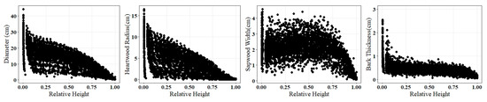
Figure 3.
Relationships between diameter, heartwood radius, sapwood radius, bark thickness, and relative height.
2.2. Methods
2.2.1. Bade Model Selection
Based on the previous literature and analysis of the relationship between the relative height and the response variable in Figure 3, the relative height and its transformation were selected as the main variables for the models. To improve the performance of the models, stand-level and tree-level variables, including Dg, Hdom, N, SI, BAS, DBH, tree age, HT, CL, and CW, were incorporated into the models using a stepwise algorithm. The best-fitting models were selected based on the Akaike information criterion (AIC) value. The form of the models was as follows:
where represents the response variable for ith observations and the kth submodels, and k refers to the heartwood radius, sapwood width, and their transformations. Value is the predictor variable, is the parameter to be estimated, and is the residual of the kth submodel.
2.2.2. Development of a Seemingly Unrelated Mixed-Effect Model System
The base linear models for profiles of heartwood, sapwood, and bark were determined. Compared to those models with plot-level, tree-level, and plot-tree-level random effects, tree-level random effects were ultimately introduced to individual mixed-effect models. Random-effect parameters were determined according to the likelihood ratio test (LRT) and AIC [27]. The individual linear mixed-effect models were merged to form a multivariate model system. Finally, a seemingly unrelated mixed-effect model with tree-level random effects was developed.
Assuming there are k individual mixed-effect models for group i, the general equation form is given as follows:
where i and j are the ith tree and jth height in the ith tree, respectively. Value k presents the kth submodels in the model system. Value is the response variable, and is the residual error for the jth height in the ith tree of the kth submodel, respectively, while and are the matrices of the fixed and random effects for the jth height in the ith tree of the kth submodel, respectively. Values are the fixed-effect parameters for the kth submodel, and are the random-effect parameters for the ith trees of the kth submodel.
The multivariate model Equation (3) can be rewritten as Equation (4).
By defining , , , , and , where , , , , and are matrices or vectors including all j elements in the ith tree.
All parameters were simultaneously estimated by the restricted maximum likelihood (REML) method [22] using the lme function in the nlme package [28] in the R environment [29], and the syntax in R of the system adjusted with the SUR method and the seemingly unrelated mixed-effect model was provided in supplementary materials.
2.2.3. Model Prediction and Local Calibration
In general, when predicting response variables using a mixed-effect model, fixed effects and random effects were considered. Only fixed-effect prediction was used if there was no local observation of response variables. If local observations were available, more information about random effects could be obtained for prediction [30]. Similarly, the seemingly unrelated mixed-effect model system allows us to use the cross-model correlations of random effects and residual errors to predict all response variables with this method. In this study, only bark thickness or three response variables were utilized for local calibration, and the estimated best linear predictor (EBLUP) was employed to estimate the predicted tree-level random effects vector and variance of prediction errors [22]. Matrices and are defined by removing from and those rows and columns that correspond to the unobserved response variables. In addition, matrix is defined by removing from all the columns that correspond to the unobserved response variables but keeping all the rows, and and are defined by removing from and those rows and columns that correspond to the unobserved response variables.
In this study, to ensure that the predicted sapwood width was positive, sapwood width on the square root scale was the response variable. Heartwood radius was predicted on its original scale by EBLUP. Hence, a bias correction factor (CF) was applied to transform sapwood width to the original scale by adding it to the square of prediction. The calculation of CF for the ith tree is as follows [22]:
where is the total variance of prediction for group i. The components of the estimation error of fixed effects and variance–covariance are ignored in Equation (7) [22].
Three alternative sampling strategies were considered for local calibrations in this study: (1) random sampling of bark for bark thickness from the whole trees with different sampling sizes (Type I), (2) sampling for bark thickness from the positions only below the 2 m height of the standing trees, i.e., four sampling points of 0 m, 1 m, 1.3 m, and 2 m to reduce labor costs and sampling difficulties (Type II), (3) sampling for heartwood radius, sapwood width and bark thickness from the positions only below the 2 m height of the standing trees with different sampling sizes, i.e., one-point sampling (1 m, 1.3 m, and 2 m), two-point sampling (1 m and 1.3 m, 1 m and 2 m, 1.3 m and 2 m), three-point sampling (1 m, 1.3 m, and 2 m), and four-point sampling (0 m, 1 m, 1.3 m, and 2 m) (Type III). In Type III, all response variables were used for local calibration; thus, , , , , and equal , , , , and in Equations (5) and (6). The unsampled points within the same tree were predicted by the three alternative strategies.
2.2.4. Model Evaluation and Validation
All data were used to fit the ordinary SUR model system and the mixed-effect SUR model system in model fitting. The adjusted coefficient of determination () and root mean square error (RMSE) [31] were calculated to evaluate and compare the fitting performance.
Prediction performance was evaluated using leave-tree-out cross-validation, which was executed n times by removing one tree from the whole dataset and using the remaining n − 1 trees for modeling [32]. In addition, the mean error (ME), mean absolute error (MAE), and (RMSE of leave-one-out cross-validation) were used for model validation and prediction performance assessment [33].
where and are the observed value and the predicted value obtained by cross-validation, respectively. and p are the numbers of observations and parameters, respectively.
3. Results
3.1. The Ordinary SUR Model System vs. Mixed-Effect SUR Model System
According to the data analysis, variable filtering, and transformation, we defined the heartwood radius, the square root of sapwood width (to ensure that the prediction was positive), and bark thickness as the final form for response variables and relative height, relative height polynomial forms, and the logarithm of relative height as the main predictors. Furthermore, DBH and age were incorporated as additional variables into the three models. Thus, the final form of ordinary SUR models was given as follows:
After comparing different-level random effects, tree-level random effects were introduced into the mixed-effect SUR models, and likelihood tests were used to select the random-effect parameter positions. Finally, the mixed-effect SUR model was determined as follows:
Parameter estimations of the ordinary SUR model system and the fixed part of the mixed-effect SUR model system are shown in Table 2. All parameters in the two model systems were significant with p values < 0.05. As shown in Table 3, all submodels in the mixed-effect SUR model system achieved better fitting performance than submodels in the ordinary SUR model system, which had lower RMSE and higher . Moreover, the heartwood radius model achieved the highest , and the sapwood width model achieved the greatest improvement in .
Table 2.
Parameter estimations of fixed effects in the ordinary seemingly unrelated model system and seemingly unrelated mixed-effect model system.
Table 3.
Fitting performance for the ordinary SUR model system and mixed-effect SUR model system.
The variance–covariance matrix of random effects in the mixed-effect SUR model system is presented in Table 4. The correlations of the random effects were between 0.309 and 0.990, and more than half were strongly correlated, indicating that the model system calibration of random effects could be achieved for local calibration. Table 5 shows the residual variance–covariance for all submodels. Strong correlations were observed between bark thickness and heartwood radius and between bark thickness and sapwood width. The heartwood radius and sapwood width had a very weak residual correlation of 0.122. The correlation between the residuals of the submodels indicated the need for simultaneous estimation in this study.
Table 4.
Variance–covariance matrix of random effects for the mixed-effect SUR model system.
Table 5.
The residual variance–covariance matrix for the mixed-effect SUR model system.
3.2. Model Validation
The performance of the mixed-effect SUR model system demonstrated its excellence in model fitting. In addition, the model’s prediction was also our concern. Table 6 compares the prediction performance of submodels using leave-one-out cross-validation between the ordinary SUR model system and the mixed-effect SUR model system. Smaller values of validation statistics (i.e., ME, MAE, and RMSE) indicated that submodels produced more reliable predictions in the mixed-effect SUR model system than in the ordinary SUR model system, especially for the sapwood width model.
Table 6.
Model system validation statistics calculated by leave-one-out cross-validation for the ordinary SUR model system and mixed-effect SUR model system. HR, SW, and BT are the heartwood radius, sapwood width, and bark thickness, respectively.
Trees were divided into four age groups: young (1–20 years), middle-aged (21–30 years), near-mature (31–40 years), and mature (41–60 years). The performance of prediction in different age groups for the submodels in the mixed-effect SUR model system was analyzed by the leave-one-out cross-validation (Figure 4). The values appear on the 45° line, indicating a close correlation between the observations and predictions. In general, the predictions showed a close correlation with their observations except for the values in the stem base, which are shown as orange points in Figure 4. For the heartwood radius model, underestimation at the stem base occurred in all age groups, and more severe underestimation occurred with increasing age. However, for the sapwood width model, severe underestimation at the base of the stem was not noticed in the near-mature group. Moreover, the bark thickness model did not show abnormal predicted values at the tree base in the young and middle-aged groups. However, the predictions at the tree base in the near-mature and mature groups were much smaller than the observations.
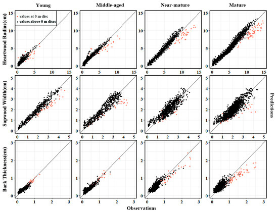
Figure 4.
Comparison of predictions and observations for heartwood radius, sapwood width, and bark thickness among different ages. The orange points represent the observations at the 0 m tree height.
The measurement points of sample trees were divided into three sections to further examine the predictability of the heartwood radius, sapwood width, and bark thickness models in the mixed-effect SUR model system (see Figure 5). For the heartwood radius model, high prediction accuracy was observed in the middle and upper sections for all age groups. In addition, in the lower section, the prediction performance worsened with increasing age. Generally, sapwood width prediction did not show a clear trend among different sections and age groups. Sapwood width in young age groups yielded better prediction than that in other age groups at each section, and sapwood width yielded a better-predicted accuracy at the middle section. The prediction of the bark thickness model did not show an obvious difference in the middle and upper sections for any age group. However, the predicted accuracy at the lower section in the near-mature and mature groups was much less than that in the young and middle-aged groups. Overall, bark thickness prediction performance in the lower (except for young and middle-aged groups) and middle sections was better than that in the upper section.
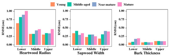
Figure 5.
Prediction accuracy by RMSE for heartwood radius, sapwood width, and bark thickness models with different age groups. A sample tree was divided into three sections by relative height (RH): lower (0 RH < 1/3), middle (1/3 RH < 2/3), and upper (2/3 RH < 1).
3.3. Model Calibration
Re-estimating random effects by EBLUP of three sampling strategies provided effectual local calibrations for the heartwood radius, sapwood width, and bark thickness. Figure 6 shows the evaluation of performance across random sampling for Type I, Type II, and Type III. The uncalibrated prediction was the prediction of the fixed effects as a reference. Type I and Type II were calibrated only by bark thickness, and Type III was calibrated by heartwood radius, sapwood width, and bark thickness. In Type I, prediction accuracy was reduced for all submodels when local observations for bark thickness were available. Greater sampling numbers generally improved the model performance but achieved lower speeds of improvement. When the number of samples reached 10, the rate of the prediction accuracy decline in the heartwood radius was already very flat, and each model achieved a significant RMSE reduction. Thus, random sampling (Type I) with 10 sampling points as one of the sampling strategies provided enough local calibration for all models.
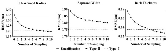
Figure 6.
Root mean square error (RMSE) for submodels of the model system. The zero number of samples represents the uncalibrated prediction.
In practice, for standing trees, it is difficult to obtain all sampling points of the whole tree. Therefore, the sampling points of the lower part of the stem (sampling points were below 2 m of the tree height) were examined in Type II and Type III. Although the sampling numbers were small, significant improvements in heartwood radius, sapwood width, and bark thickness prediction were observed in Type II compared with the uncalibrated prediction. However, the improvements in sapwood width and bark thickness were lower than random sampling with a sampling size of 10. Figure 7 compares the prediction performance with different sizes and different sampling points below 2 m of the tree height in Type III. Since Type III models were calibrated with all response variables, the heartwood radius and sapwood width prediction accuracies greatly improved and were much higher than those of the other sampling strategies. However, there was no obvious difference between the sample size and sampling points for heartwood radius and sapwood width. The bark thickness predictive accuracy varied with different sample sizes and points, and it obtained the best prediction in four-point sampling.
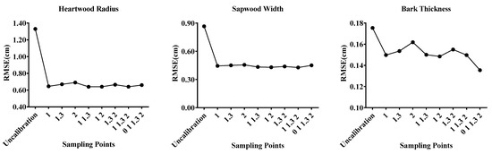
Figure 7.
The calibrated prediction for submodels of the model system in Type III.
4. Discussion
The variation in the profiles of heartwood, sapwood, and bark along the stem was analyzed to select predictor variables and model forms. The results (Figure 3) suggested that the heartwood radius and bark thickness decreased from base to top for the trees of Korean larch among various ages and sites, which agreed with the results of studies for other species [15,34,35,36]. In contrast to previous findings [2,4,9,37], sapwood width was higher at the tree base, increased above the tree base to the maximum at the living branch height, and then decreased with tree height. According to the analysis, the linear model form was determined for the heartwood radius and sapwood width model as in previous studies [8,10,19]. Moreover, relative height and its transformations were selected as the main predictor variable, which is similar to the findings of Flæte and Høibø [10] for Scot pine that heartwood diameter was related to the vertical positions in the tree. Predictor variables such as diameter over bark, heartwood radius at breast height, and sapwood width at breast height [8,19] did not consider destructive samples. In addition, many different forms are available as alternatives for bark thickness models, such as the quadratic regression equation, polynomial regression equation [38], segmented polynomial regression equation [39], variable exponent equation [40], and a combination of the stem taper function and bark thickness model by Yang and Radtke [15]. Relative height was the main predictor in these models, as in our study. Considering the relatively uniform model form in the model system and predictive performance, the linear bark thickness model form was finally determined. Furthermore, more explanatory variables, i.e., diameter outside the bark, breast height diameter, and tree age were suggested to increase predictive accuracy in the studies by Stängle et al. [12] and Stängle and Dormann [13]. However, due to the difficulty of obtaining the diameter outside bark at any height, DBH and tree age was finally chosen as explanatory variables in practical applications. Therefore, all predictor variables in the model system were easy-to-measure variables, and their measurements did not damage the trees. The purpose of developing a forest model is to apply it in the forestry practice. Hence, utilizing easily-measured variables in the model was essential in this study.
Profiles of heartwood, sapwood, and bark were measured on the same disc of the same tree; thus, they were modeled simultaneously by a SUR technique in this study. Moreover, the results (Table 5) showed that the residual correlation across models was significant, which indicated that it is preferred to apply SUR modeling to reduce the standard error of parameter estimation and total uncertainties [25]. Mixed-effect models improve modeling performance and efficiency by reflecting the variation between individuals for hierarchical structure data. When introducing random effects into the models, plot-level, tree-level, and plot-tree-level random effects were considered and tested. The plot-level random effects provided much less model fitting improvement than tree-level and plot-tree-level random effects, and models with plot-tree-level random effects did not improve significantly compared to the models with tree-level random effects. Therefore, tree-level random effects were introduced in the models, which could reflect tree genetic characteristics, social status, and micro standing sites. The submodels in the mixed-effect SUR model system significantly improve the fitting performance compared to the ordinary SUR model system (Table 3). The promotion and high accuracy in heartwood radius models were consistent with the linear mixed-effect models constructed by Wilhelmsson et al. [19] and Flæte and Høibø [10]. The sapwood width model achieved great improvement by applying random effects, demonstrating large individual variation. Little research focuses on modeling sapwood width along the stem; thus, the sapwood width model in this study could provide a model possibility. The bark thickness model also effectively improved the model fitting performance, as in previous findings [11,12]. In addition, the results showed that all response variables in the mixed-effect SUR model system were well fitted by relative height, DBH, and age, indicating that the profiles of heartwood, sapwood, and bark could be fitted well by linear models and fewer variables compared to more complex models.
Consistent with the fitting accuracy, the prediction accuracy of submodels in mixed-effect SUR models was higher than the ordinary SUR model system, as shown in Table 6. The submodel predictions of the mixed-effect SUR model system performed well under different age groups (Figure 4). However, the excessive underestimation at the base of the tree was obvious, especially in the near-mature and mature groups. Butt swell of trees and the irregular heartwood growth of different directions in this area may be responsible for this result [8]. Additionally, we analyzed the prediction accuracy of heartwood radius, sapwood width, and bark thickness at different sections in different age groups (Figure 5). We found that much of the prediction error for heartwood radius came from the lower section of the stem. Based on the results in Figure 4, the larger errors existed at the tree base, where the heartwood radius of four directions was irregular, which may be associated with the butt swell. This trend was found in parametric and nonparametric stem taper models for Betula platyphylla [41]. Overall, sapwood width predictions exhibited similar performance at different sections of the tree in different age groups, and its prediction accuracy did not show a trend at different sections. The sapwood width model in the young age group showed better accuracy than that in other age groups for each section, which proved that the sapwood model in this study was more suitable for young age groups. This may be associated with regular and small sapwood for young trees, and the polynomial regression equation could describe the young tree sapwood width shape well. Moreover, the bark thickness prediction accuracy at the lower section in the near-mature and mature groups was much higher than that in other sections in different age groups, as shown in Figure 4, where the predicted bark thickness at the stem base was much smaller than the observed values in the near-mature and mature groups. This is because older trees have much larger bark at the base of the tree than other parts of the tree [18].
In addition to the good fitting performance of the mixed-effect SUR model system in this study, the greatest benefit of the model system was the improvement in the practical application achieved by providing local calibration. Although there are mixed-effect models for predicting heartwood radius and sapwood width at different heights of the tree, the model calibration has not been examined due to the destructive samples. In this paper, simultaneous modeling calibrating random effects and residuals provided a good solution by calibrating heartwood radius and sapwood width with bark thickness, which made the newly observed samples only require the bark thickness without destroying the internal structure of the tree. The influence of sampling strategy and size on estimating the random effects has been studied [24,32,42]. Three effectual strategies with different sizes were examined and discussed in our study. The results (Figure 6) showed that the prediction of heartwood radius and sapwood width could be calibrated effectively in Type I and Type II, which proved that calibrating only by bark thickness significantly improved the accuracy of random effects. Due to the different variation patterns of the stem between sapwood width and bark thickness, the random-effect correlation between sapwood width and bark thickness in the mixed-effect SUR model system was not as strong as the correlation between heartwood radius and bark thickness. Thus, the prediction accuracy improvement of sapwood width in Type I was smaller than that in Type II, which was different from heartwood radius and bark thickness. The models calibrated by all response variables (Type III) presented the highest prediction accuracy in all sampling strategies (Figure 7). Moreover, Type III compared the difference in sample size and sampling points on prediction performance. The heartwood radius and sapwood width exhibited similar good predictive accuracy at all sampling sizes and points; thus, one-point sampling was suggested as a method for their model calibration. However, the prediction of bark thickness varied with different sampling sizes and points. The best predictive accuracy in four-point sampling proved that sampling at a height of 0 m played an important role in the prediction accuracy of the lower part of the model. In practice, the sampling strategy of Type III could be realized by sampling from the tree cores below the 2 m height of the tree, but the tree core at 0 m tree height was harder to obtain than other heights. Therefore, considering the cost and damage to trees, one-point sampling at a tree height of 1 m was suggested for our mixed-effect model system in Type III. Overall, the three sampling strategies in this study provided adequate prediction accuracy in estimating the random effects of the models. Furthermore, the three different sampling strategies can be applied in different scenarios. Measuring bark thickness at any height in standing trees is difficult and costly, and it can destroy the integrity of the bark; this may result in direct contact between the interior of the stem and the outside world, which can lead to damage or even death by fire, insects, and infection [43,44]. Therefore, random sampling (Type I) could be used for felled trees in the timber industry to ensure the integrity of the tree’s internal structure, and it also provides information on the distribution of sapwood and heartwood of trees. Sampling for bark thickness under the 2 m height of the tree (Type II) and sampling for all response variables at 0 m of the tree height (Type III) are suggested for standing trees to keep them alive for sustainable management of forestry as well as improve the prediction accuracy. The prediction performance of Type II was worse than that of other sampling strategies, but it only needs four-point sampling for bark thickness.
The model system in this study could quantify the profiles of heartwood, sapwood, and bark well and be effectively calibrated by bark thickness. However, the radius of the stem was not considered in the model system. Therefore, the additivity property and the true taper models for stem profiles were the limitations of this study., which will be considered in future research.
5. Conclusions
In this study, the seemingly unrelated mixed-effect approach was utilized to quantify the profiles of heartwood, sapwood, and bark simultaneously. Relative height and its transformation, which is easy to measure, were chosen as the main predictors, and DBH and tree age were chosen as covariates to improve the predictions. In addition, bark thickness and all response variables were used to calibrate heartwood radius and sapwood width by the random-effect correlation of submodels in the seemingly unrelated mixed-effect model system. Three different sampling strategies were provided for different scenarios: random sampling for bark thickness, sampling for bark thickness below the 2 m height of the tree, and sampling for response variables below the 2 m height of the tree. The heartwood radius, sapwood width, and bark thickness models in the model system achieved good improvements in model fitting and prediction accuracy except for the base of the stem compared with the ordinary seemingly unrelated model system. In addition, all models in the model system improved prediction accuracy after calibration with three sampling strategies. A random sampling of bark thickness with a sampling size of 10 was suggested for felled trees to understand the timber volume distributed in heartwood and sapwood, in addition to the bark volume, and to keep the complete stem structure and volume in the timber industry, and sampling for bark thickness below the 2 m height of the tree was preferred for standing trees to keep trees active for sustainable management of forestry. Sampling for all response variables below the 2 m height of the tree greatly improved the prediction accuracy, but at a cost of more serious damage than that of other strategies. The results in this study indicated that applying a seemingly unrelated mixed-effect model could effectively improve the fitting accuracy of the heartwood radius, sapwood width, and bark thickness and predict heartwood radius and sapwood width without disruptive sampling for the stem, which is a benefit for the sustainable development and rational utilization of wood in forest management.
Supplementary Materials
The following supporting information can be downloaded at: https://www.mdpi.com/article/10.3390/f14061216/s1.
Author Contributions
Conceptualization, L.D. and F.L.; data curation, Y.Q.; formal analysis, Y.Q., Y.H., L.D. and F.L.; funding acquisition, L.D. and F.L.; methodology, L.D. and F.L.; project administration, L.D. and F.L.; resources, Y.Q., L.D. and F.L.; software, Y.Q. and Y.H.; supervision, S.-I.Y., L.D. and F.L.; validation, Y.Q., S.-I.Y., Y.H., Z.M., L.D. and F.L.; visualization, Y.Q.; writing—original draft, Y.Q.; writing—review and editing, Y.Q., S.-I.Y., Y.H., Z.M., L.D. and F.L. All authors have read and agreed to the published version of the manuscript.
Funding
This research was funded by the Natural Science Foundation of China (U21A20244) and Fundamental Research Funds for the Central Universities of Ministry of Education of China (No. 2572020DR03).
Data Availability Statement
The data presented in this study are available on request from the corresponding author. The data are not publicly available due to confidentiality.
Acknowledgments
The authors would like to thank the faculty and students of the Department of Forest Management, Northeast Forestry University (NEFU), China who provided and collected the data for this study.
Conflicts of Interest
The authors declare no conflict of interest.
References
- Climent, J.; Chambel, M.R.; Pérez, E.; Gil, L.; Pardos, J. Relationship between Heartwood Radius and Early Radial Growth, Tree Age, and Climate in Pinus canariensis. Can. J. For. Res. 2002, 32, 103–111. [Google Scholar] [CrossRef]
- Pinto, I.; Helena, P.; Usenius, A. Heartwood and Sapwood Development within Maritime Pine (Pinus pinaster Ait.) Stems. Trees 2004, 18, 284–294. [Google Scholar] [CrossRef]
- Wiedenhoeft, A.C. Structure and Function of Wood. In Handbook of Wood Chemistry and Wood Composite, 2nd ed.; Taylor & Francis: Oxford, UK, 2012; pp. 9–32. [Google Scholar] [CrossRef]
- Knapic, S.; Tavares, F.; Pereira, H. Heartwood and Sapwood Variation in Acacia Melanoxylon R. Br. Trees in Portugal. Forestry 2006, 79, 371–380. [Google Scholar] [CrossRef]
- Nawrot, M.; Pazdrowski, W.; Szymański, M. Dynamics of Heartwood Formation and Axial and Radial Distribution of Sapwood and Heartwood in Stems of European Larch (Larix decidua Mill.). J. For. Sci. 2008, 54, 409–417. [Google Scholar] [CrossRef]
- Pâques, L.E. Genetic Control of Heartwood Content in Larch. Silvae Genet. 2001, 50, 69–75. [Google Scholar]
- Bektas, I.; Hakki Alma, M.; Goker, Y.; Yuksel, A.; Gundogan, R. Influence of Site on Sapwood and Heartwood Ratios of Turkish Calabrian Pine. For. Prod. J. 2003, 53, 48–50. [Google Scholar]
- Climent, J.; Chambel, M.R.; Gil, L.; Pardos, J.A. Vertical Heartwood Variation Patterns and Prediction of Heartwood Volume in Pinus canariensis Sm. For. Ecol. Manag. 2003, 174, 203–211. [Google Scholar] [CrossRef]
- Yang, K.C.; Hazenberg, G.; Bradfield, G.E.; Maze, J.R. Vertical Variation of Sapwood Thickness in Pinus banksiana Lamb. and Larix laricina (Du Roi) K. Koch. Can. J. For. Res. 1985, 15, 822–828. [Google Scholar] [CrossRef]
- Flæte, P.O.; Høibø, O. Models for Predicting Vertical Profiles of Heartwood Diameter in Mature Scots Pine. Can. J. For. Res. 2009, 39, 527–536. [Google Scholar] [CrossRef]
- Li, R.; Weiskittel, A.R. Estimating and Predicting Bark Thickness for Seven Conifer Species in the Acadian Region of North America Using a Mixed-Effects Modeling Approach: Comparison of Model Forms and Subsampling Strategies. Eur. J. For. Res. 2011, 130, 219–233. [Google Scholar] [CrossRef]
- Stängle, S.M.; Sauter, U.H.; Dormann, C.F. Comparison of Models for Estimating Bark Thickness of Picea Abies in Southwest Germany: The Role of Tree, Stand, and Environmental Factors. Ann. For. Sci. 2017, 74, 16. [Google Scholar] [CrossRef]
- Stängle, S.M.; Dormann, C.F. Modelling the Variation of Bark Thickness within and between European Silver Fir (Abies alba Mill.) Trees in Southwest Germany. Forestry 2018, 91, 283–294. [Google Scholar] [CrossRef]
- Mosaffaei, Z.; Jahani, A. Modeling of Ash (Fraxinus excelsior) Bark Thickness in Urban Forests Using Artificial Neural Network (ANN) and Regression Models. Model. Earth Syst. Environ. 2021, 7, 1443–1452. [Google Scholar] [CrossRef]
- Yang, S.-I.; Radtke, P.J. Predicting Bark Thickness with One- and Two-Stage Regression Models for Three Hardwood Species in the Southeastern US. For. Ecol. Manag. 2022, 503, 119778. [Google Scholar] [CrossRef]
- Zeibig-Kichas, N.E.; Ardis, C.W.; Berrill, J.P.; King, J.P. Bark Thickness Equations for Mixed-Conifer Forest Type in Klamath and Sierra Nevada Mountains of California. Int. J. For. Res. 2016, 2016, 28–31. [Google Scholar] [CrossRef]
- Fernández-Sólis, D.; Berrocal, A.; Moya, R. Heartwood Formation and Prediction of Heartwood Parameters in Tectona grandis L. f. Trees Growing in Forest Plantations in Costa Rica. Bois For. Trop. 2018, 335, 25–37. [Google Scholar] [CrossRef]
- Costa, A.; Barbosa, I.; Pestana, M.; Miguel, C. Modelling Bark Thickness Variation in Stems of Cork Oak in South-Western Portugal. Eur. J. For. Res. 2020, 139, 611–625. [Google Scholar] [CrossRef]
- Wilhelmsson, L.; Arlinger, J.; Spångberg, K.; Lundqvist, S.O.; Grahn, T.; Hedenberg, Ö.; Olsson, L. Models for Predicting Wood Properties in Stems of Picea abies and Pinus sylvestris in Sweden. Scand. J. For. Res. 2002, 17, 330–350. [Google Scholar] [CrossRef]
- Laasasenaho, J.; Melkas, T.; Aldén, S. Modelling Bark Thickness of Picea abies with Taper Curves. For. Ecol. Manag. 2005, 206, 35–47. [Google Scholar] [CrossRef]
- Longuetaud, F.; Mothe, F.; Leban, J.M.; Mäkelä, A. Picea abies Sapwood Width: Variations within and between Trees. Scand. J. For. Res. 2006, 21, 41–53. [Google Scholar] [CrossRef]
- Lauri Mehtätalo, J.L. Biometry for Forestry and Environmental Data with Examples in R; CRC Press: Boca Raton, FL, USA, 2020; ISBN 977-2-08141-5. [Google Scholar]
- Maltamo, M.; Mehtätalo, L.; Vauhkonen, J.; Packalén, P. Predicting and Calibrating Tree Attributes by Means of Airborne Laser Scanning and Field Measurements. Can. J. For. Res. 2012, 42, 1896–1907. [Google Scholar] [CrossRef]
- Bronisz, K.; Mehtätalo, L. Seemingly Unrelated Mixed-Effects Biomass Models for Young Silver Birch Stands on Post-Agricultural Lands. Forests 2020, 11, 381. [Google Scholar] [CrossRef]
- Hao, Y.; Widagdo, F.R.A.; Liu, X.; Quan, Y.; Liu, Z.; Dong, L.; Li, F. Estimation and Calibration of Stem Diameter Distribution Using UAV Laser Scanning Data: A Case Study for Larch (Larix olgensis) Forests in Northeast China. Remote Sens. Environ. 2022, 268, 112769. [Google Scholar] [CrossRef]
- State Forestry and Grassland Administration. The Ninth Forest Resource Survey Report (2014–2018); State Forestry and Grassland Administration: Beijing, China, 2019. [Google Scholar]
- Akaike, H. Information Theory and an Extension of the Maximum Likelihood Principle. In Selected Papers of Hirotugu Akaike; Springer: New York, NY, USA, 1998; pp. 199–213. [Google Scholar]
- Pinheiro, J.; Bates, D.; DebRoy, S.; Sarkar, D. R Core Team Nlme: Linear and Nonlinear Mixed Effects Models; R Core Team: Vienna, Austria, 2020. [Google Scholar]
- R Core Team. R: A Language and Environment for Statistical Computing; R Core Team: Vienna, Austria, 2020. [Google Scholar]
- Lappi, J. Calibration of Height and Volume Equations with Random Parameters. For. Sci. 1991, 37, 781–801. [Google Scholar]
- Dong, L.; Zhang, L.; Li, F. A Compatible System of Biomass Equations for Three Conifer Species in Northeast, China. For. Ecol. Manag. 2014, 329, 306–317. [Google Scholar] [CrossRef]
- Temesgen, H.; Monleon, V.J.; Hann, D.W. Analysis and Comparison of Nonlinear Tree Height Prediction Strategies for Douglas-Fir Forests. Can. J. For. Res. 2008, 38, 553–565. [Google Scholar] [CrossRef]
- Ciceu, A.; Garcia-Duro, J.; Seceleanu, I.; Badea, O. A Generalized Nonlinear Mixed-Effects Height–Diameter Model for Norway Spruce in Mixed-Uneven Aged Stands. For. Ecol. Manag. 2020, 477, 118507. [Google Scholar] [CrossRef]
- Herrero de Aza, C.; Turrión, M.B.; Pando, V.; Bravo, F. Carbon in Heartwood, Sapwood and Bark along the Stem Profile in Three Mediterranean Pinus Species. Ann. For. Sci. 2011, 68, 1067–1076. [Google Scholar] [CrossRef]
- Sousa, V.B.; Cardoso, S.; Pereira, H. Ring Width Variation and Heartwood Development in Quercus faginea. Wood Fiber Sci. 2013, 45, 405–414. [Google Scholar]
- Zhao, Z.; Shen, W.; Wang, C.; Jia, H.; Zeng, J. Heartwood Variations in Mid-Aged Plantations of Erythrophleum fordii. J. For. Res. 2021, 32, 2375–2383. [Google Scholar] [CrossRef]
- Cardoso, S.; Pereira, H. Characterization of Douglas-Fir Grown in Portugal: Heartwood, Sapwood, Bark, Ring Width and Taper. Eur. J. For. Res. 2017, 136, 597–607. [Google Scholar] [CrossRef]
- Cao, Q.V.; Pepper, W.D. Predicting Inside Bark Diameter for Shortleaf, Loblolly, and Longleaf Pines. South. J. Appl. For. 1986, 10, 220–224. [Google Scholar] [CrossRef]
- Max, T.A.; Burkhart, H.E. Segmented Polynomial Regression Applied to Taper Equations. For. Sci. 1976, 22, 283–289. [Google Scholar]
- Kozak, A. My Last Words on Taper Equations. For. Chron. 2004, 80, 507–515. [Google Scholar] [CrossRef]
- He, P.; Jiang, L.; Li, F. Evaluation of Parametric and Non-Parametric Stem Taper Modeling Approaches: A Case Study for Betula Platyphylla in Northeast China. For. Ecol. Manag. 2022, 525, 120535. [Google Scholar] [CrossRef]
- Crecente-Campo, F.; Tomé, M.; Soares, P.; Diéguez-Aranda, U. A Generalized Nonlinear Mixed-Effects Height–Diameter Model for Eucalyptus globulus L. in Northwestern Spain. For. Ecol. Manag. 2010, 259, 943–952. [Google Scholar] [CrossRef]
- Ferrenberg, S.; Mitton, J.B. Smooth Bark Surfaces Can Defend Trees against Insect Attack: Resurrecting a “slippery” Hypothesis. Funct. Ecol. 2014, 28, 837–845. [Google Scholar] [CrossRef]
- Pausas, J.G. Bark Thickness and Fire Regime. Funct. Ecol. 2015, 29, 315–327. [Google Scholar] [CrossRef]


Disclaimer/Publisher’s Note: The statements, opinions and data contained in all publications are solely those of the individual author(s) and contributor(s) and not of MDPI and/or the editor(s). MDPI and/or the editor(s) disclaim responsibility for any injury to people or property resulting from any ideas, methods, instructions or products referred to in the content. |
© 2023 by the authors. Licensee MDPI, Basel, Switzerland. This article is an open access article distributed under the terms and conditions of the Creative Commons Attribution (CC BY) license (https://creativecommons.org/licenses/by/4.0/).