Article

The Importance of Using Permanent Plots Data to Fit the Self-Thinning Line: An Example for Maritime Pine Stands in Portugal

by
Muha Abdullah Al Pavel
*,
Susana Barreiro
and
Margarida Tomé
Forest Research Centre, Associated Laboratory TERRA, School of Agriculture, University of Lisbon, Tapada da Ajuda, 1349-017 Lisbon, Portugal
*
Author to whom correspondence should be addressed.
Forests 2023, 14(7), 1354; https://doi.org/10.3390/f14071354
Submission received: 21 May 2023 / Revised: 26 June 2023 / Accepted: 28 June 2023 / Published: 30 June 2023
(This article belongs to the Section Forest Ecology and Management)

Abstract

:
Density-dependent mortality occurs in the evolution of even-aged populations when these approach crown closure age. This density-dependent mortality is regulated by the so-called “3/2 power law of self-thinning” that assumes a constant slope for the line relating the log of stand density with the log of the average tree size, the self-thinning line or maximum size–density relationship, MSDR. A good estimate of the self-thinning line is therefore an essential component to any forest growth model. Two concepts for the MSDR have emerged: (1) a static upper limit for the species; and (2) a dynamic self-thinning line influenced by several factors (e.g., management techniques, site quality and/or genetics). The objective of this study was to estimate a new static self-thinning line based on the quadratic mean diameter at breast height (Reineke’s self-thinning line) for the generalized use in maritime pine growth models in Portugal. Data from 41 observations obtained in nine long-term permanent experimental trials of maritime pine species were carefully selected from a data set of 186 plots as being under self-thinning. Two methods were used: OLS and mixed linear models. An exploratory analysis on the impact of each environmental variable on the slope and intercept of the self-thinning line led to the selection of a subset of environmental variables later used in an all possible regressions algorithm to find the subsets leading to the lowest values of Akaike information criterion (AIC). The OLS procedure showed that the differences between the plots could be explained by site index, by climate variables (e.g., evaporation or climatic indices) and the use of more than one covariable slightly improved the fit. Nevertheless, the best MSDR line fitted with mixed linear models (ln N = 12.97158 − 1.83926 ln dg) having the plot random effect in the intercept, largely outperformed the best OLS model and is therefore recommended for generalized use in forest growth models.

1. Introduction

Maritime pine (Pinus pinaster Aiton.) is the third most representative tree species in terms of area coverage in Portugal, occupying 714 thousand ha, which is equivalent to 23 percent of the total forest land in the country [1]. The species provides the second most important material for the wood industry, an important industrial sector in Portugal, with a harvest of ca. 4.4 million m3 in 2020 [2] and a value of 0.7 million Euros of exports, 1.2% of total Portuguese exports and 16% of total forest exports [3].
The importance of the species in the Portuguese forest sector leads to the need to optimize forest management, which requires the use of forest growth models that simulate the dynamics of forest stands over time, considering both the constructive (growth) and destructive (mortality and harvest) mechanisms. Two types of mortality can be considered: density-dependent mortality and mortality caused by biotic and abiotic events (e.g., pests and diseases, storms, wildfires) [4]. Density-dependent mortality results from inter-tree competition and is therefore an essential component of a forest growth model (e.g., Burkhart and Tomé [5]).
Most Mediterranean pine stands regenerate well by natural regeneration, among them maritime pine that is adapted to natural regeneration after fire [6,7]. Naturally regenerated stands can have very high densities of seedlings, as high as 7500–90,000 trees ha−1, achieving crown closure at a young age [8]. When growing taller and bigger, trees in forests compete strongly for available resources including light, water, and nutrients as well as for space. The weaker trees will inevitably be suppressed and die under minimal resource allocation [9]. It is widely agreed [10,11] that density-dependent mortality occurs in the evolution of monospecific even aged plant populations that are fully crown-closed. This density-dependent mortality is regulated by the “3/2 power law of self-thinning” initially formulated by Yoda et al. [12] who, examining thinning in overcrowded pure populations of several species on soils of varying fertility and found that the number of surviving plants could be related to their mean weight as w = C.p−3/2, where p is the density of surviving plants and w their corresponding mean weight [10]. Intraspecies-driven natural mortality plays an important role in species dynamics and controls natural density evolution [13]. The relationship between maximum plant density and average plant size explains this dynamic [12,14]. The model supports the setting for the theoretical limit of the number of trees for a certain average tree dimension [8,12]. Reineke [14] expressed the self-thinning line as a linear relationship between the logarithm of stand density (N, number of plants per unit of area) and the logarithm of the quadratic mean diameter at breast height (dg), ln N = ln k + a ln dg, where k and a are, respectively, the intercept and slope for the model. In forestry, when fitting the self-thinning line, the quadratic mean diameter is usually used as the size of the average tree. A typical slope of −1.605 has been assumed by Reineke [14] as valid for a large variety of species in full stocked stands. Self-thinning modeling [15,16] and the resulting stand-density diagrams [17,18] have been established more for the Pinus genus, than for any other genus.
Many authors (e.g., [15,17,19,20,21,22]) fitted this model for species growing in diverse environments finding other slope values. Analyses reveal that, considering the differences in self-tolerance, shadow resistant species have a lower slope [13] and a higher intercept [23]. Some studies [9,24,25] found that the shift in the trajectory and/or the maximum density value depends on the aspect of the stands and on the characteristics of the environment. Deviance from the straight line is often found [21,26,27]. This deviation can take place at both ends of the line, in young stands before competition starts and, later, in old stands induced by reduction in self-tolerance [13], which leads to a concave curve [8,28]. Over the entire range of stand development, the relationship between ln N and ln dg is then curvilinear and only the intermediate stage is linear. Henceforth, the term self-thinning line will be used to refer to the intermediate stage, the most relevant for growth models.
There has been debate around the constancy of the self-thinning slope among different stands of the same species (discussed for instance in VanderSchaaf and Burkhart [28]). In the sequence of these discussions, two concepts for the maximum size–density relationship have emerged: (1) a static upper limit for the species; and (2) a dynamic thinning line, with intercept and slope values varying among stands, influenced by several factors as, for instance, management techniques, site quality and genetics. The authors proposed a refinement of the static MSDR species boundary line by defining two MSDR species boundary lines: (I) with a slope that results from positioning the boundary above all observations without accounting for self-thinning patterns of individual stands; and (II) with a slope that can be considered the population average of all MSDR dynamic thinning lines. Using data from a loblolly pine spacing trial, VanderSchaaf and Burkhart [28] fitted type II static maximum size–density relationships (MSDR) to the linear part of the relationship between ln N and ln dg comparing three methodologies: ordinary least squares (OLS), first-difference models and linear mixed-effects models. These authors concluded that the linear mixed-effects model, by considering the within-plot autocorrelation, reflected the average population mean better. Additionally, this method was also the one that produced the most stable estimates along a gradient of spacings.

The Self-Thinning Line for Maritime Pine

Oliveira, [19] developed the first self-thinning line for maritime pine in Portugal, using data from a small set of temporary plots and proposed the equation ln N = 11.418 − 1.516 ln dg. Later on, Luís and Fonseca [22], using 274 temporary plots measured in the fourth Portuguese National Forest Inventory, defined a new self-thinning line. However, none of these slope values have been validated against data from permanent plots, the only way to guarantee the accuracy of the estimated slope value. Tomé [29] used ordinary least squares to fit a self-thinning line with data from unthinned permanent plots, selecting the maximum observed stand density for each quadratic mean diameter, therefore following a type I MSDR and not considering the dynamic MSDR lines for each permanent plot.
The self-thinning of maritime pine stands in Spain was first studied by del Río et al. [30] that, using data from temporary plots established in unthinned stands and classified as having maximum density, estimated a slope of −1.605. Later, Riofrío et al. [31] used data from two consecutive National Forest Inventories (cycle of 10 years) with mortality rates between inventories that indicated self-thinning conditions and log-linear quantile regression to obtain the slope and intercept of the self-thinning line of pure maritime pine stands, considering the 95th quantiles. Charru et al. [32], based on the French National Forest Inventory data, studied the self-thinning relationships for 11 species, among which was maritime pine, using a ‘stochastic frontier’ technique. Before fitting the self-thinning line, the authors rejected plots having a quadratic mean diameter < 15 cm and plots with very low mortality. Table 1 summarizes the values of the intercept and slope for all of these models, showing also the corresponding SDI values (for a reference dg of 25 cm) to show the relationship between the self-thinning lines and stand density at a reference dg. Figure 1 compares the several self-thinning lines: Charru et al. [32] and Oliveira [19] lines are much lower than the other lines while Luís and Fonseca [22] is the model allowing a larger stock. In what concerns the slopes two groups can be identified: del Río et al. [30] and Oliveira [19] against the other ones (Charru et al. [32] is intermediate between the two groups). There are large differences in the self-thinning lines that have been developed for maritime pine, which justifies the need for deeper research on this topic. Additionally, all of the above referred MSDR lines are type I lines, while our objective was to develop a population average type II MSDR for the species.
The need for this study emerged after using the data available for maritime pine growth in Portugal from long-term measurements in experimental plots—with a number of remeasurements from 3 to 17 years and a duration of measurement from 2 to 31 years—to evaluate the previously published self-thinning lines. This analysis showed a large variability among the existing curves and indicated the need to use this data to estimate a new self-thinning line for generalized use in growth models for this species in Portugal. As in VanderSchaaf and Burkhart [28], the main objective of this study was to obtain new estimates for the slope and intercept of a static MSDR applicable to all the stands of this species in Portugal, defined as the fixed part of a linear mixed model (population mean). A second objective was to identify some site factors that may be related to the variation of the intercept and/or slope of the dynamic self-thinning lines.

2. Materials and Methods

2.1. Data

Data for this study originates from maritime pine experimental trials from Portugal (Table 2), including different types of trials (spacing, thinning and pruning trials). The objective was to select from the whole sets of data, unthinned plots as well as other plots with high stand densities, at least during part of the stand life (the period used for each plot varied between 2 to 10 years). All data available were pre-processed in order to obtain the number of trees per ha (N) and the quadratic mean diameter (dg) (Reineke’s self-thinning line).
In order to explore possible impacts of environmental variables on the self-thinning line, each plot was characterized in terms of: site index (S), estimated with the site index curves from Tomé [29]; climatic variables, 1971–2000 averages obtained from the closest clipick [33] grid point: temperature (temp), precipitation (prec), relative humidity (hum), evaporation (evap); lithology and soil type, obtained from the Portuguese “Atlas do Ambiente” (SNIAmb, accessed in [34]). The climatic variables were also combined in some aridity indices often used in forest growth modeling: Martonne, Lang and Meyer (for definitions see, e.g., [35,36,37,38]):
Martonne = prec/(temp + 10),
Lang = prec/temp,
Meyer = prec/{100 − (hum/100 temp)},
The dry period (dryp), defined as the number of months with precipitation less than 40 mm, was also used as a possible explanatory variable. As the number of trials is small using lithology and soil type were coincident, therefore we just used soil type for our analysis. Podzols and cambisols were the only soil types present in the selected trials, a dummy variable (cambi) was used to represent the cambisols soil type.
The following procedure was used in order to select the plots-measurements corresponding to self-thinning stands:
  • For an overall pre-analysis, the data from the whole dataset were initially plotted together. Three of the self-thinning lines found in the literature, selected as representing well the spread among the different lines, were also plotted just for comparison: Luís and Fonseca [22]; Tomé [29] and Charru et al. [32].
  • Then, the data for each trial were plotted jointly with the three self-thinning lines selected and, by examining the graphs, the trials with no evidence of self-thinning were discarded.
  • In the remaining trials, all the non-thinned plots (e.g., control plots from the thinning trials) were selected.
  • For each selected plot, graphs of ln N versus ln dg were created to assess whether the trajectories approached an MSDR dynamic thinning line boundary. A comparison with the three self-thinning lines referred in 1. helped deciding.
  • Following the methodology used by VanderSchaaf and Burkhart [28] all the selected plots were visually assessed and only those points occurring along an MSDR dynamic thinning line boundary were selected, often eliminating the initial measurements of the plots. A plot was included in the analysis if there were at least two consecutive points along an MSDR dynamic thinning line.
  • During this procedure, some of the trials or measurements previously selected in 4. were discarded. The final data set, containing just plots in a self-thinning stage, was used to fit the self-thinning line.

2.2. Estimating the MSDR Species Boundary Line Coefficients

As a starting point, an exploratory analysis of the environmental variables that might influence the self-thinning line was made using ordinary least squares (OLS). First, one analysis was undertaken for each of the continuous variables available, testing the significance of adding the variable to either the intercept, the slope or both. A similar analysis was made for the categorical variable soil type using the dummy variable cambi. The variables and/or interactions between variables with a higher impact were then used in the analysis using the “olsrr” R package [39] for all possible regressions in order to obtain the subsets of variables with the lowest values of Akaike information criterion (AIC).
In a second stage, and following VanderSchaaf and Burkhart [28] that verified the superiority of the linear mixed effects method to fit the MSDR static line, this method was used to fit the self-thinning line for maritime pine in Portugal.
The linear mixed-effects model can be expressed as:
Yi = Xi β + Zi bi + εi
where Yi is the matrix with the data of ln dgi, Xi β is the fixed part of the model, Zi bi is the random part and εi is the unexplained information or model error. Xi and Zi are design matrices, including ln dg and environmental variables and the interactions of environmental variables with ln dg (depending on each specific model), of dimension ni × p and ni × q, respectively, where ni is the number of observations, p is the number of explanatory variables in Xi and q the number of explanatory variables in Zi. The assumptions for the linear mixed model are:
  • bi~N (0, D)
  • εi~N (0, ∑i)
  • b1, , bn, ε1, , εn are independent.
The superiority of using linear-mixed models relates to its ability to take into account the correlation of the numerous points from the same cluster [28]. Our dataset has a hierarchical structure with two clusters: the trials and the plots inside the trials. Thus, several alternatives for the structure of random effects were tested in the process of selecting the best models considering the two clusters, just the trials or just the plots. Several alternative models were tested considering different structures for the clusters and random effects. Zuur et al. [40] recommends that the random structure of a mixed model must be selected starting from as many explanatory variables as possible in the fixed component. Because the set of environmental variables was large and strong multicollinearity was observed, the initial fixed component was defined based on the results of the all possible regressions algorithm previously used to select the best OLS models. The open-source statistical software R, version 4.2.2 [41] and packages “lme4” [42] and “lmer” [42] function were used in this analysis. Several random structures considering plots within trials or just plots as random effects were added, included just in the intercept, in the slope or in both.
The comparison between the alternative models and therefore the selection of the final model was based on the AIC statistic (other statistics of model performance were also computed). The regression assumptions, namely the normality of the residuals and heteroscedasticity, were assessed in the selected models by graphical analysis of the QQ-plots and of the studentized residuals versus the estimated values, respectively.

3. Results

The maritime pine data from Portuguese trials strongly showed the idea of a maximum for the relationship between ln N and ln dg (Figure 2). Two groups of trials/plots data can be identified in the graph: the group represented by the more or less horizontal lines that are far away from the self-thinning line (correspond to plantations) and the group represented by steep lines that is close to the maximum line (self-thinning). Two groups of trials/plots data can be identified in the graph: the group represented by the more or less horizontal lines that are far away from the self-thinning line (correspond to plantations) and the group represented by steep lines that is close to the maximum line (self-thinning).
Figure 3a shows the evolution of the ln N vs. ln dg line for all the control (unthinned) plots of the selected trials. As can be observed, there are some plots that still have not reached the self-thinning stage and some plots for which the first points (first measurements) are still away from the self-thinning line that must also be eliminated. The final plots/measurements selected to fit the self-thinning line can be seen in Figure 3b. Some differences among the plots can be clearly seen, especially in what concerns the intercept of the self-thinning line.
Table 3 summarizes the results of fitting the alternative OLS models showing, for each environmental variable, the model (among the models with the covariate in the intercept, in the slope or in both) that gave the best results in terms of the AIC. Site index (S) and evaporation (evap), both with impact on the intercept, appear as the environmental variables with a bigger influence on the self-thinning line. Higher site indices are associated with lower intercepts, while higher values of evaporation are associated with higher intercepts.
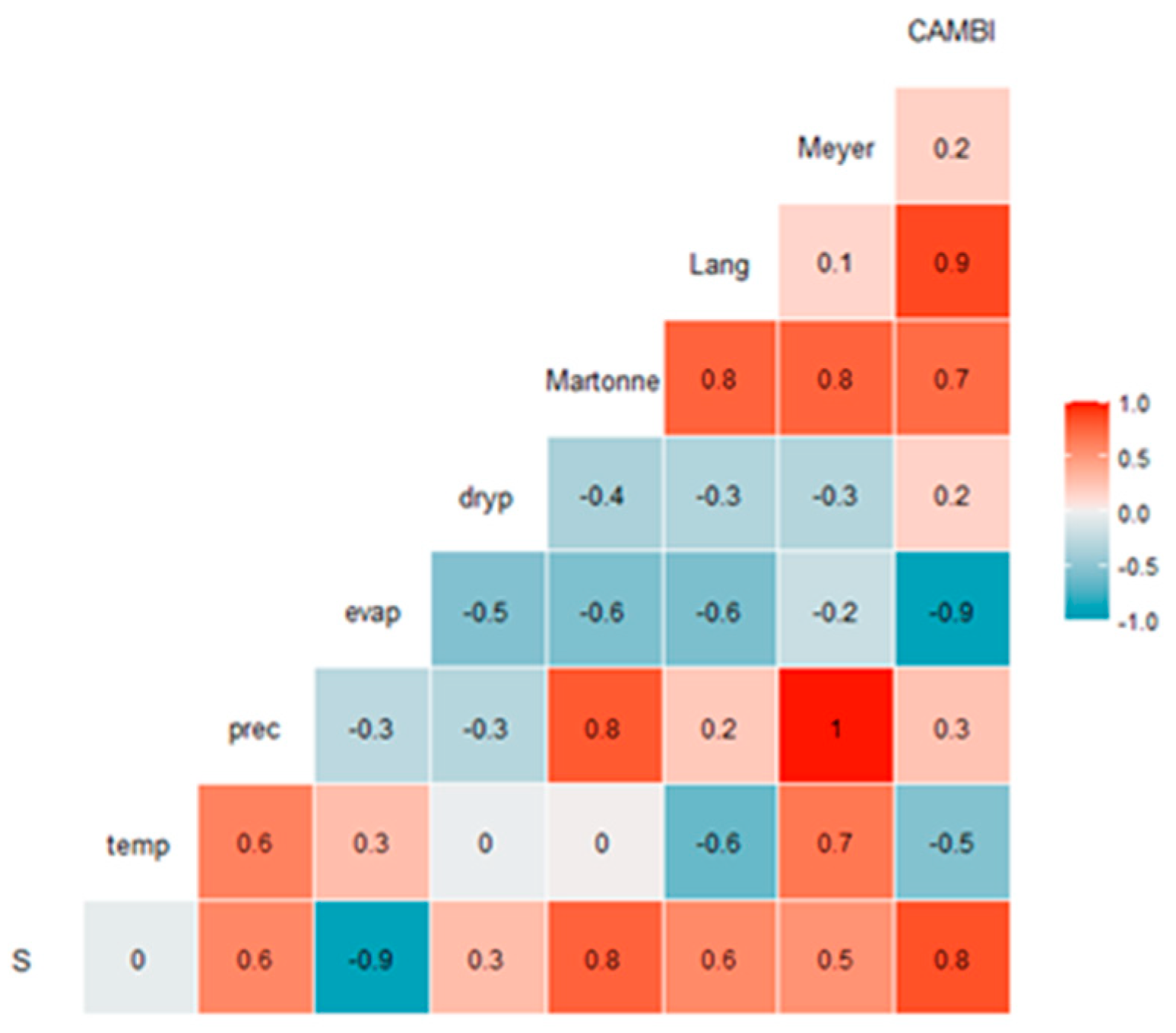
The environmental variables used as possible regressors were highly correlated (Figure 4), justifying the use of the all possible regressions algorithm to find subsets of environmental variables leading to models with a good performance. Table 4 shows the results of the best 10 OLS models obtained with the all possible regressions algorithm (Table S1 shows other model performance criteria). Some of the models including certain subsets of variables outperformed the best OLS models including just one covariable. Nonetheless, the improvements in the AIC values were not substantial and some of the selected models evidenced either high values for variance inflation factors (VIF), which indicate multicollinearity, or the existence of parameters not differing significantly from zero (Table 4). Overall, several of the models had a good performance, including low variance inflation factors values. The best models usually included one of the climatic indices (Meyer or Martonne). The dry period (dryp), not highly correlated with the climatic indices, is one of the variables in several of the best models.
Models Ols.0 (without environmental variables), Ols.S (with site index in the intercept) and Ols.evap (with evap in the intercept) were also tested as alternatives for the fixed part. Table 5 shows the results for all the models tested, including some models with not all the parameters significantly different from zero, as well as the respective simplified versions with all parameters significantly different from zero. The models with random effects in the slope usually did not converge. The analysis of the AIC values with other goodness-of-fit statistics (Table S1) showed that considering the effect of plots within trials was not superior to simply considering the effect of plots in the intercept.
The analysis of Table 3, Table 4 and Table 5 shows that the model Mix2.0—mixed model with the random effect of plot in the intercept—is the one that provides the best static self-thinning line for generalized use in growth and yield models. The variance of the plot random effect represents more than 90% of the total residual variance. This model, shown in Table 6, was therefore selected for generalized use in forest growth models.
Table 3 and Table 4 allow the selection of some OLS models that might be used to estimate the self-thinning line of a particular stand. Models Ols.S, Ols.evap and Ols.allpr.1 are useful for this type of application if model simplicity, AIC and maximum VIF are taken into consideration. The first two are the best models with just one variable and the third is the best model resulting from the all possible regressions. The model with evap instead of S may be a good alternative when age is not available. Note that most of the best models obtained with the all possible regression (Ols.allpr.1, to Ols.allpr.4), include the variable dry period (dryp), one of the aridity indices (Meyer or Martonne) and some other climatic variable.
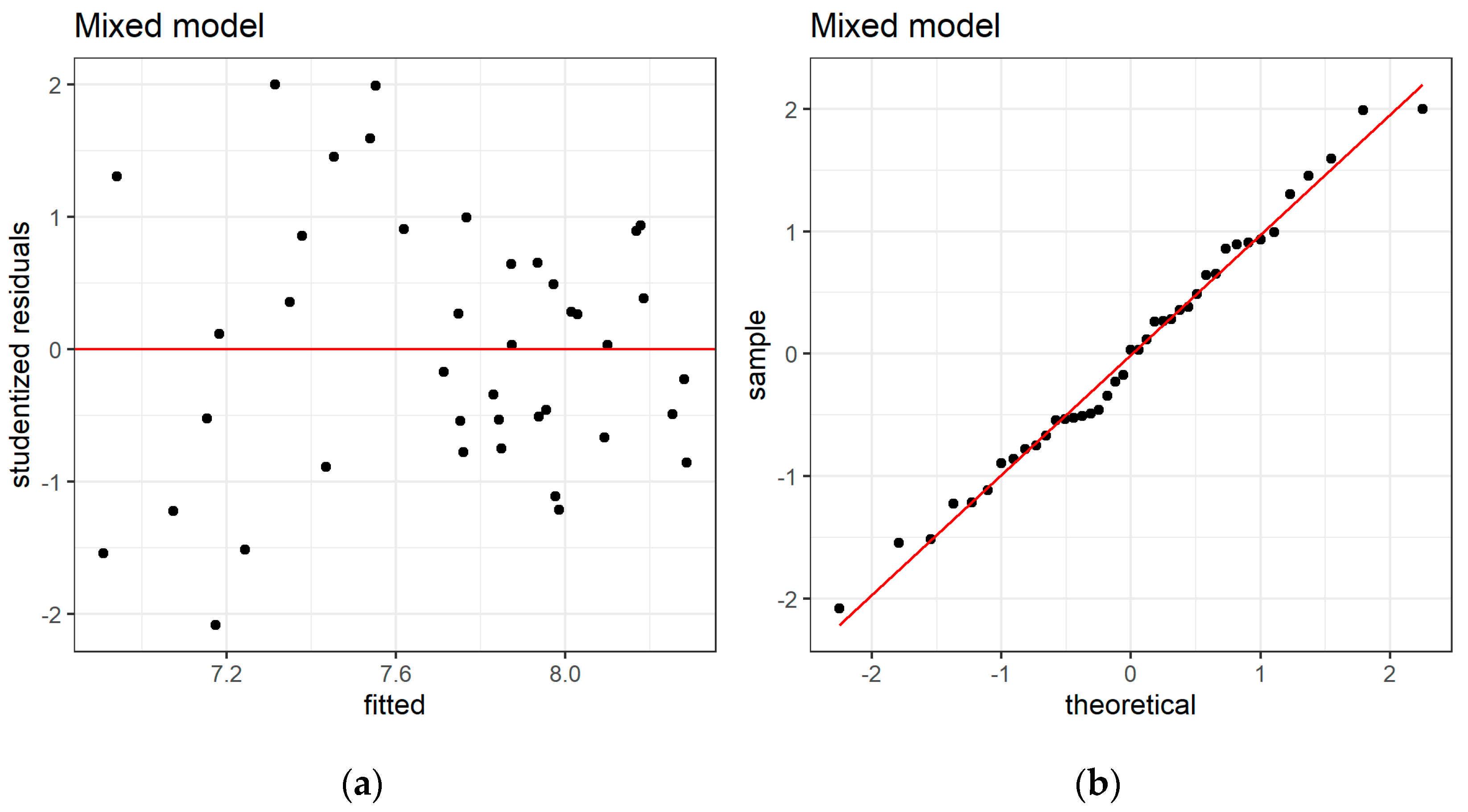
The verification of the regression assumptions for the selected model showed no relevant deviations from the normality and constant variance of the residuals was found (Figure 5). The same analysis was made for the Ols models proposed and the results for the homoscedasticity of variance were similar, but the qq-plots had tails slightly deviating from the normal line, but not too much.
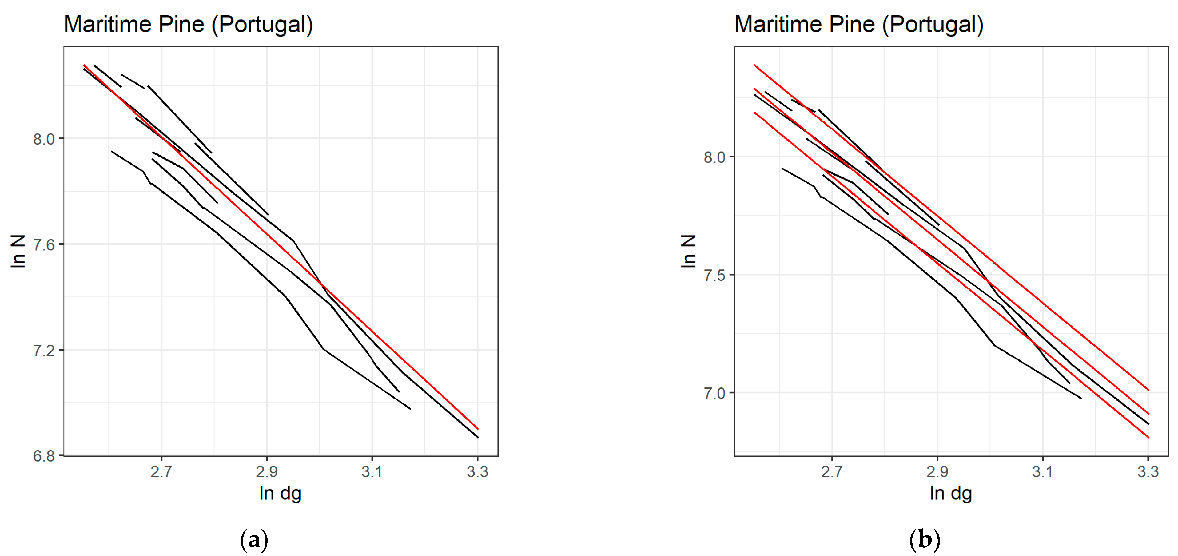
Figure 6 shows the plot of the selected model Mix2.0 and of the Ols.0.S model jointly with the observed data. The Mix2.0 model (Figure 6a) provides a static MSDR self-thinning line that represents an average line for all plots under self-thinning while the Ols.0.S (Figure 6b) adapts the line to each plot according to the respective site index.

4. Discussion

This research used data from permanent plots to obtain a static self-thinning line (also called maximum size–density relationship, MSDR) for generalized use in forest growth models of maritime pine in Portugal. The need for such study arose after comparing the existing self-thinning lines fitted for this species and finding large differences among them (Figure 1). A second objective was to identify whether some environmental variables could explain part of the variation of the intercept and/or slope of the dynamic self-thinning lines.
The number of trials and plots available for the study was reasonable (11 trials with 186 plots, n = 1338), although the number reduced drastically (five trials and nine plots, n = 85) after the thinned plots were eliminated. The difficulty in having a large number of unthinned permanent plots is common and has been experienced by other authors. For instance, Pretzsch and Biber [43] used 29 plots, with long time series, to study the MSDR of four tree species.
Most of the maritime pine self-thinning lines previously developed [19,22,29,30,31,32] differed among themselves and also from the ones developed in this research. For the intercept values ranged from 11.418 to 13.634 and for the slope from −1.516 to −1.956. The differences may derive from the data sets used in the fitting procedure but also from the methodology adopted in each case. Most of the existing self-thinning curves were developed using temporary plots measured under the framework of the National Forest Inventories (NFI), or not taking advantage of existing permanent plots. Therefore, the objective was to fit an equation close to the data points that, for each dg value, had the highest N (maximum density points—MDP), being therefore type I lines. Some authors achieved the goal selecting those MDP points by different methods [19,22,29,30] and fitting the line with ordinary least squares. Methods vary from a subjective selection of the points with higher density [19], to the selection of the higher point for each dg class [29], to a boundary point definition [22] or the selection of unthinned plots of high density [30]. Over the last decade, more sophisticated statistical techniques were used such as the ‘stochastic frontier’ technique [32] or log-linear quantile regression, taking the 95% quantile as the self-thinning line [31]. The later authors had two measurements in each NFI, but they only used those to assess if the plots had a high decrease in the number of trees per ha, most likely because it is difficult to understand whether the decreasing number of trees per ha in NFI plots is really due to self-thinning or to management. In fact, this may be the reason why the intercept obtained by Charru et al. [32] is the lowest: maritime pine in France is mainly planted and managed, therefore the MDP obtained from the NFI plots may not correspond to self-thinning.
On the other hand, the method used to fit the self-thinning line should also be chosen carefully as it will have a high influence on the estimation of the slope. For instance, using our data set after deleting points corresponding to very young stands, far away from the self-thinning line (n = 879), to fit a self-thinning line with quantile regression (99%), led to an intercept of 13.5131 and a slope of −1.9952. However, applying the same methodology to NFI5 Portuguese data for the pure even-aged maritime pine stands (n = 622), an intercept of 11.5027 and a slope of −1.4112 were obtained. The values from the two data sets are considerably different, and the intercepts and slopes are different from those obtained with linear-mixed model techniques. These results show the importance of using data from permanent plots in order to obtain unbiased estimates. Of course, the number of permanent plots under self-thinning available for this type of studies is usually small as long-term plots often suffer some disturbance resulting in shorter time series than desired. As mentioned by Pretzsch and Biber [43], stand dynamics under self-thinning conditions is particularly informative under eco-physiological and production economics aspects as it reveals the species-specific critical demand for resources and the growing space of average trees of a given size.
Even if the number of trials and plots was small we investigated if there were some environmental variables that could be used to estimate dynamic maximum density lines. Site index (S) or evaporation (evap), when added to the model intercept, most contributed to improve model performance, as evaluated by the AIC criteria. Using the all possible regressions algorithm allowed finding models with three environmental variables slightly better than the models with just one environmental variable. Condés et al. [37] also found that the Martonne aridity index added to the intercept and slope of the self-thinning line improved model performance for the species studied (European beach, Fagus sylvatica L., and Scots pine, Pinus sylvestris L.). The impact of climate on the two species was not the same: for European beach, the higher the humidity, the steeper the MSDR (more negative exponent) and the higher the intercept, while for Scots pine, the higher the humidity, the higher (less negative) the exponent and the lower the intercept. In our case, larger values of site index also implied a smaller intercept. However, other studies [44,45] had opposite results with the stands growing on the more productive sites having larger intercept values. The variables that may influence the intercept and slope values of the self-thinning line are multiple and the number of observations available to fit those lines are usually small, which makes the interpretation of the estimates obtained with different data sets and different methodologies difficult. This justifies the preference for using data collected in unthinned permanent plots, because these exhibit the real MSDR line.
Using data from a loblolly pine spacing trial, VanderSchaaf and Burkhart [28] fitted type II static maximum size–density relationships (MSDR) to the linear part of the relationship between ln N and ln dg comparing three methodologies: ordinary least squares; first-difference models and linear mixed-effects models. They concluded that the linear mixed-effects model better reflected the average population mean by taking into account the within-plot autocorrelation. This conclusion was similar to our finding that the mixed model with the plot random effect in the intercept outperformed, based on the AIC statistic, the best ordinary least squares models. The best mixed model, representing an average MSDR line for the species, did not include environmental variables.
The main objective of this study was to obtain an average self-thinning line for generalized use in forest growth and yield models. The average line cannot be considered as an absolute biological maximum, and therefore the results of this study cannot be used for this purpose, as that will require other fitting techniques to be explored in future studies.

5. Conclusions

The previously reported Reineke’s self-thinning lines for maritime pine (Pinus pinaster Aiton.) were re-evaluated with data from 186 permanent plots from 12 trials and a new model for generalized use in growth models of maritime pine species in Portugal, developed using the subset of unthinned plots (nine plots within five trials) and mixed models’ techniques, was proposed (Table 6). The slope estimate is −1.83926, with a confidence interval of [−1.898495; −1.781555], therefore being statistically different from the Reineke’s proposed value of −1.605. The static self-thinning line corresponds to an SDI value of 1154. The dynamic thinning lines, representing the variation among self-thinning lines of individual plots, were modeled using the impact of environmental variables in the intercept or in the intercept and slope (Table 6).
This study also proves the importance of using permanent plots data to study the stands’ self-thinning dynamics and therefore points to the need to establish permanent plots in unthinned stands to be monitored in the long-term.
The nature of the slope for a static MSDR for stand development, and the knowledge about the maximum size–density relationship line is essential to identify the best silvicultural prescriptions and management options for the Portuguese maritime pine forest system. The results achieved are relevant for generalized use in growth models.

Supplementary Materials

The following supporting information can be downloaded at: https://www.mdpi.com/article/10.3390/f14071354/s1, Table S1: The best 10 OLS models without environmental variables and the best models with just one variable are included for comparative purposes based on basic statistics.

Author Contributions

Conceptualization and methodology, M.A.A.P., S.B. and M.T.; data curation, M.A.A.P., S.B. and M.T.; writing—original draft preparation, M.A.A.P.; writing—review and editing, M.A.A.P., S.B. and M.T.; supervision, S.B. and M.T. All authors have read and agreed to the published version of the manuscript.

Funding

This research was funded by the Fundação para a Ciência e a Tecnologia I. P. (FCT), Portugal, co-financed by the European Union (EU), through the PhD program on Climate Change and Sustainable Development Policies (PDACPDS), M.A.A.P. doctoral grant (SFRH/PD/BD/135442/2017); by the exceptional doctoral grant (COVID/BD/152046/2021). The Fundação para a Ciência e a Tecnologia has also supported the research through S.B. framework contract nr 1382 (DL57/2016/CP1382/CT0026).

Data Availability Statement

Not applicable.

Acknowledgments

The authors are grateful to the colleagues and staff who assisted with the Maritime pine forest inventory data from Portugal making the data available for the analysis. This research was supported by the Forest Research Centre, a research unit funded by Fundação para a Ciência e a Tecnologia I.P. (FCT), Portugal (UIDB/00239/2020), and by the Associated Laboratory TERRA (LA/P/0092/2020). The authors are also thankful to the support provided by the Forest Carbon Flux and Storage Mapping Service European project (H2020-SPACE-2018-2020, Grant Agreement number: 821860). Finally, the authors would like to thank the reviewers for their valuable comments that contributed to improving the manuscript.

Conflicts of Interest

The authors declare no conflict of interest.

References

  1. ICNF. 6.o Inventário Florestal Nacional (IFN6)—2015 Relatório Final; ICNF: Lisboa, Portugal, 2019.
  2. INE. Estatísticas Agrícolas—2021; INE: Lisboa, Portugal, 2022.
  3. INE. Estatísticas de Comércio Internacional—2019. Available online: https://www.ine.pt/xportal/xmain?xpid=INE&xpgid=ine_publicacoes&PUBLICACOESpub_boui=133545&PUBLICACOESmodo=2 (accessed on 27 December 2022).
  4. Vanclay, J.K. Modelling Forest Growth and Yield: Applications to Mixed Tropical Forests, 1st ed.; CAB International: Wallingford, UK, 1994; ISBN 0851989136.
  5. Burkhart, H.E.; Tomé, M. Quantifying Stand Density. In Modeling Forest Trees and Stands; Springer: Dordrecht, The Netherlands, 2012; pp. 175–200. [Google Scholar]
  6. Tapias, R.; Climent, J.; Pardos, J.A.; Gil, L. Life histories of Mediterranean pines. In The Plant Ecology; Springer: Berlin/Heidelberg, Germany, 2004; Volume 171, pp. 53–68. [Google Scholar]
  7. Maia, P.; Keizer, J.; Vasques, A.; Abrantes, N.; Roxo, L.; Fernandes, P.; Ferreira, A.; Moreira, F. Post-fire plant diversity and abundance in pine and eucalypt stands in Portugal: Effects of biogeography, topography, forest type and post-fire management. For. Ecol. Manag. 2014, 334, 154–162. [Google Scholar] [CrossRef]
  8. Enes, T.; Lousada, J.; Aranha, J.; Cerveira, A.; Alegria, C.; Fonseca, T. Size–density trajectory in regenerated maritime pine stands after fire. Forests 2019, 10, 1057. [Google Scholar] [CrossRef] [Green Version]
  9. Brunet-Navarro, P.; Sterck, F.J.; Vayreda, J.; Martinez-Vilalta, J.; Mohren, G.M.J. Self-thinning in four pine species: An evaluation of potential climate impacts. Ann. For. Sci. 2016, 73, 1025–1034. [Google Scholar] [CrossRef] [Green Version]
  10. White, J.; Harper, J.L. Correlated Changes in Plant Size and Number in Plant Populations. J. Ecol. 1970, 58, 467. [Google Scholar] [CrossRef]
  11. Smith, N.J.; Hann, D.W. A growth model based on the self-thinning rule. Can. J. For. Res. 1986, 16, 330–334. [Google Scholar] [CrossRef]
  12. Yoda, K.; Kira, T.; Ogawa, H.; Hozumi, K. Self-thinning in overcrowded pure stands under cultivated and natural conditions. J. Biol. 1963, 14, 107–129. [Google Scholar]
  13. Zeide, B. Analysis of the 3/2 Power Law of Self-Thinning; Oxford Academic: Oxford, UK, 1987; Volume 33. [Google Scholar]
  14. Reineke, L.H. Perfecting a stand-density index for even-aged forests. J. Agric. Res. 1933, 46, 627–638. [Google Scholar]
  15. von Gadow, K. Observations on self-thinning in pine plantations. S. Afr. J. Sci. 1986, 82, 364–368. [Google Scholar]
  16. White, J. The allometric interpretation of the self-thinning rule. J. Theor. Biol. 1981, 89, 475–500. [Google Scholar] [CrossRef]
  17. McCarter, J.B.; Long, J.N. A Lodgepole Pine Density Management Diagram. West. J. Appl. For. 1986, 1, 6–11. [Google Scholar] [CrossRef]
  18. Dean, T.J.; Jokela, E.J. A Density-Management Diagram for Slash Pine Plantations in the Lower Coastal Plain. South. J. Appl. For. 1992, 16, 178–185. [Google Scholar] [CrossRef]
  19. Oliveira, A.C. Tabela de Produção Geral Para o Pinheiro Bravo das Regiões Montanas e Sub-Montanas; Direção Geral das Florestas/Centro de Estudos Florestais (INIC): Lisboa, Portugal, 1985. [Google Scholar]
  20. Dean, T.; Baldwin, V.C.J. Using a Density-Management Diagram to Develop Thinning Schedules for Loblolly Pine Plantations. Res. Pap. SO-275 1993, 275, 12. [Google Scholar]
  21. Cao, Q.V.; Dean, T.J.; Baldwin, V.C. Modeling the size-density relationship in direct-seeded slash pine stands. For. Sci. 2000, 46, 317–321. [Google Scholar]
  22. Luis, J.F.S.; Fonseca, T.F. The allometric model in the stand density management of Pinus pinaster Ait. in Portugal. Ann. For. Sci. 2004, 61, 807–814. [Google Scholar] [CrossRef] [Green Version]
  23. Harper, J.L. Population Biology of Plants; Academic Press: Cambridge, NY, USA, 1977; ISBN 0123258502. [Google Scholar]
  24. Aguirre, A.; del Río, M.; Condés, S. Intra- and inter-specific variation of the maximum size-density relationship along an aridity gradient in Iberian pinewoods. For. Ecol. Manag. 2018, 411, 90–100. [Google Scholar] [CrossRef]
  25. Andrews, C.; Weiskittel, A.; D’Amato, A.W.; Simons-Legaard, E. Variation in the maximum stand density index and its linkage to climate in mixed species forests of the North American Acadian Region. For. Ecol. Manag. 2018, 417, 90–102. [Google Scholar] [CrossRef]
  26. Zeide, B. A relationship between size of trees and their number. For. Ecol. Manag. 1995, 72, 265–272. [Google Scholar] [CrossRef]
  27. Fonseca, T.; Monteiro, L.; Enes, T.; Cerveira, A. Self-thinning dynamics in cork oak woodlands: Providing a baseline for managing density. For. Syst. 2017, 26, e006. [Google Scholar] [CrossRef] [Green Version]
  28. VanderSchaaf, C.L.; Burkhart, H.E. Comparison of methods to estimate Reineke’s maximum size-density relationship species boundary line slope. For. Sci. 2007, 53, 435–442. [Google Scholar]
  29. Tomé, M. Tabela de Produção Geral Para o Pinheiro Bravo em Portugal; Universidade Técnica de Lisboa: Lisboa, Portugal, 2001. [Google Scholar]
  30. del Río, M.; Lopez-Senespleda, E.; Montero, G. Manual de Gestión Para Masas Procedentes de Repoblación de Pinus pinaster Ait, Pinus sylvestris L. y Pinus nigra Arn. en Castilla y León; Consejería de Medio Ambiente, Junta de Castilla y León: León, Spain, 2006. [Google Scholar]
  31. Riofrío, J.; del Río, M.; Bravo, F. Mixing effects on growth efficiency in mixed pine forests. Forestry 2016, 90, 381–392. [Google Scholar] [CrossRef] [Green Version]
  32. Charru, M.; Seynave, I.; Morneau, F.; Rivoire, M.; Bontemps, J.D. Significant differences and curvilinearity in the self-thinning relationships of 11 temperate tree species assessed from forest inventory data. Ann. For. Sci. 2012, 69, 195–205. [Google Scholar] [CrossRef] [Green Version]
  33. Palma, J. CliPick—Climate change web picker. A tool bridging daily climate needs in process based modelling in forestry and agriculture. For. Syst. 2017, 26, 2171–9845. [Google Scholar]
  34. SNIAmb Visualizador SNIAmb—Atlas—Atlas do Ambiente. Available online: https://sniamb.apambiente.pt/content/geo-visualizador?language=pt-pt (accessed on 3 April 2023).
  35. Araujo, K.D.; De Andrade, A.P.; Cavalcanti, R.W. GEOAMBIENTE ON-LINE. 2008. Available online: https://revistas.ufg.br/geoambiente/issue/view/1373 (accessed on 3 April 2023).
  36. Martonne, E. Une Nouvelle Fonction CIimatologique: L’Indice d’Aridite (A New CIimatological Function: The Aridity Index). La Météorologie 1926, 2, 449–458. [Google Scholar]
  37. Condés, S.; Vallet, P.; Bielak, K.; Bravo-Oviedo, A.; Coll, L.; Ducey, M.J.; Pach, M.; Pretzsch, H.; Sterba, H.; Vayreda, J.; et al. Climate influences on the maximum size-density relationship in Scots pine (Pinus sylvestris L.) and European beech (Fagus sylvatica L.) stands. For. Ecol. Manag. 2017, 385, 295–307. [Google Scholar] [CrossRef]
  38. Paulo, J.A.; Firmino, P.N.; Tomé, M. A tree- and climate-dependent growth model to predict mature annual cork thickness under different climate change scenarios. Model. Earth Syst. Environ. 2023, 2023, 1–14. [Google Scholar] [CrossRef]
  39. Hebbali, A. R Package “Olsrr”, Version 0.5.3; Tools for Building OLS Regression Models; 2022. Available online: https://olsrr.rsquaredacademy.com/ (accessed on 3 April 2023).
  40. Zuur, A.F.; Ieno, E.N.; Walker, N.J.; Saveliev, A.A.; Smith, G.M. Mixed Effects Models and Extensions in Ecology with R; Springer: Berlin/Heidelberg, Germany, 2009; ISBN 978-0-387-87457-9. [Google Scholar]
  41. R Core Team. R: A Language and Environment for Statistical Computing; R Found Statistical Computing: Vienna, Austria, 2022; p. 2. Available online: https://www.R-project.org (accessed on 27 December 2022).
  42. Bates, D.; Mächler, M.; Zurich, E.; Bolker, B.M.; Walker, S.C. Fitting Linear Mixed-Effects Models Using Lme4. J. Stat. Softw. 2015, 67, 1–48. [Google Scholar] [CrossRef]
  43. Pretzsch, H.; Biber, P. A re-evaluation of Reineke’s rule and stand density index. For. Sci. 2005, 51, 304–320. [Google Scholar]
  44. Bi, H. Stochastic frontier analysis of a classic self-thinning experiment. Austral Ecol. 2004, 29, 408–417. [Google Scholar] [CrossRef]
  45. Weiskittel, A.; Gould, P.; Temesgen, H. Sources of variation in the self-thinning boundary line for three species with varying levels of shade tolerance. For. Sci. 2009, 55, 84–93. [Google Scholar]
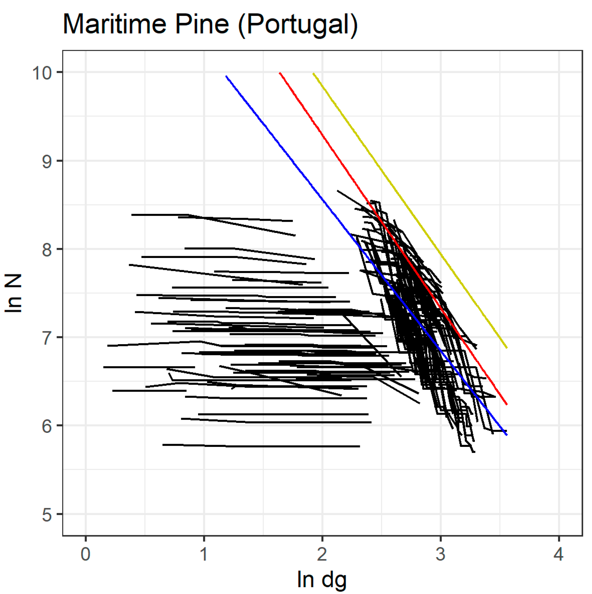
Figure 1. Self-thinning lines available in the literature for maritime pine [19,22,29,30,31,32].
Forests 14 01354 g001
Figure 2. ln N − ln dg relationship for the maritime pine permanent plots in Portugal (black lines represent trials/plots observed data). Some of the existing self-thinning lines are also represented: the upper yellow (Luís and Fonseca [22]), middle red (Tomé [29]) and bottom blue (Charru et al. [32]).
Forests 14 01354 g002
Figure 3. MSDR trajectories of all the 14 control plots (a) and of the nine plots selected to fit the self-thinning line (b) (number of observations equal to 85 and 41, respectively, for (a,b). Different trials represented by different colors.
Forests 14 01354 g003
Figure 4. Correlation between environmental variables used as possible regressors in the OLS models.
Forests 14 01354 g004
Figure 5. Plots of the studentized residuals versus fitted values (a) and qq-plot of the studentized residuals (b) for the selected model Mix2.0. (mixed model with the plot random effect in the intercept).
Forests 14 01354 g005
Figure 6. Relationship of ln N − ln dg for the self-thinning plots (in black); including the selected MSDR species boundary line in red (a) and the dynamic MSDR lines for three site indices: (base age = 50 years): 15 (lower, SDI = 1295), 20 (middle, SDI = 1172) and 25 (upper, SDI = 1060) in red (b).
Forests 14 01354 g006
Table 1. Self-thinning lines for maritime pine stands in the Iberian peninsula.
Author(s)CountryRegionInterceptSlopeSDI 1
Oliveira [19]PortugalMontanas e sub-montanas11.418−1.516691
Tomé [29]PortugalWhole country13.200−1.956996
Luís and Fonseca [22]PortugalWhole country13.634−1.8971859
del Río et al. [30]SpainCastilla y León12.562−1.6051629
Charru et al. [32]FranceWhole country, NFI data 211.982−1.711648
Riofrío et al. [31]SpainWhole country, NFI data 313.218−1.9291106
1 for reference dg = 25 cm; 2 three consecutive NFI; 3 two consecutive NFI.
Table 2. Characteristics of the plots used in this study, considering the initial data set and the data set corresponding to plots and measurements selected to fit the self-thinning line.
Whole Data Set (12 Trials, 186 Plots, n = 1338)Self-Thinning Data Set (5 Trials, 9 Plots, n = 41)
VariablesMinMeanMaxSdMinMeanMaxSd
t2.0020.6150.0010.8624.0032.7850.005.76
hdom0.3810.4526.355.7012.4617.6125.493.63
dg0.0012.3935.247.6812.8317.1927.163.49
N30014569796105096024193930842
G0.0019.6164.0816.4240.7850.6660.065.22
S15.3120.8728.392.7616.7723.2525.492.86
temp8.712.314.91.768.710.811.81.27
prec685.51096.41412.7231.11093.71260.31363.1125.7
hum71.476.879.73.171.977.379.33.2
evap1.01.32.40.41.01.31.50.2
dryp2.73.44.20.52.72.73.60.4
Martonne27.650.066.0113.252.160.565.24.9
Lang46.092.7132.929.299.4117.0132.912.7
Meyer7.712.115.52.511.913.814.91.5
t = Age (years); hdom = dominant height (m); dg = quadratic mean diameter (cm); N = number of trees (trees/ha); G = basal area (m2/ha); and S = site index (m); temp = temperature; prec = precipitation; hum = relative humidity; evap = evaporation. dryp = dry period as the number of months with precipitation less than 40 mm.
Table 3. Models fitted to the self-thinning data set with ordinary least squares, considering just one environmental variable as a possible covariate indicating the respective parameters estimates and adjusted R2 and AIC as performance criteria. Just the best model for each covariate is shown.
Covariate (X)Parameter EstimatesResidual
Variance
Adjusted R2AIC
Interceptln dgXX × ln dg
none13.2282−1.9479--0.10660.924−63.24
S13.3822−1.8377−0.0200-0.09330.942−73.31
temp35.1886−10.1429−2.03240.75750.10000.933−66.69
prec12.9643−1.5978--−0.01930.10060.932−67.05
evap12.6842−1.86620.2808-0.09440.940−72.29
dryp13.1863−1.77068-(.) −0.05490.10410.927−64.29
Martonne13.0227−1.5781-−0.00470.10130.931−66.52
Lang(ns) −9.0987(.) 6.39470.1780−0.06660.10180.930−65.18
Meyer13.5972−1.8689−0.0409-0.10170.931−66.22
cambi13.0888−1.8721-−0.03370.10070.932−66.97
ln dg = the natural logarithm of quadratic mean diameter; S = site index (base age = 50 years); temp = temperature; prec = precipitation; evap = evaporation; dryp = dry period as the number of months with precipitation less than 40 mm; Martonne, Lang and Meyer = aridity indices; cambi = cambisols soil type; AIC = Akaike information criterion; (.) = the parameter was significant just at p < 0.1; ns = the parameter was not significantly different from zero.
Table 4. Best 10 OLS models obtained with the all possible regressions algorithm. The model without environmental variables as well as the best models with just one variable are also included for comparative purposes.
Model IDVariables in the ModelMax (VIF)AIC
InterceptSlope
Ols.0-ln dg-−63.24
Ols.SSln dg1.16−73.31
Ols.evapevapln dg1.09−72.29
Ols.allpr.1dryp Meyerln dg prec3.14−77.39
Ols.allpr.2Meyerln dg prec, ln dg dryp7.68−77.32
Ols.allpr.3evapln dg dryp, ln dg Martonne1.74−77.27
Ols.allpr.4-ln dg evap, ln dg dryp, ln dg Martonne1.56−77.17
Ols.allpr.5templn dg temp, ln dg evap 2.81−77.07
Ols.allpr.6-ln dg, ln dg temp, ln dg evap3.07−76.91
Ols.allpr.7temp evapln dg temp3.30−76.88
Ols.allpr.8-ln dg evap, ln dg Lang, ln dg cambi66.33−76.88
Ols.allpr.9templn dg, ln dg evap1.24−76.87
Ols.allpr.10evapln dg, ln dg temp3.31−76.82
ln dg = the natural logarithm of quadratic mean diameter; S = site index (base age = 50 years); temp = temperature; prec = precipitation; evap = evaporation; dryp = dry period as the number of months with precipitation less than 40 mm; Martonne, Lang and Meyer = climate index; cambi = cambisols soil type; Max (VIF) = the maximum value of the variance inflations factors; AIC = Akaike information criterion.
Table 5. Models fitted to the self-thinning data set with linear mixed models, considering alternatives as the fixed part with the respective AIC value as a performance criteria.
Model IDFixed PartRandom PartAICRandom Effects VarianceResidual Variance
Groups
Mix1.all.possOls.allpos.1(1|Trial)−51.980.00460.0068
Mix2.all.possOls.allpos.1(1|Plot)−108.120.00710.0009
Mix3.all.possOls.allpos.1(1|Trial/Plot)−106.140.0065; 0.00100.0009
Mix4.all.possOls.allpos.1(1 + ln dg|Trial)No conv--
Mix5.all.possOls.allpos.1(1 + ln dg|Trial/Plot)No conv--
Mix1.0Ols.0(1|Trial)−65.390.00710.0068
Mix2.0Ols.0(1|Plot)−118.980.01130.0010
Mix3.0Ols.0(1|Trial/Plot)−118.660.0056; 0.05670.0010
Mix4.0Ols.0(1 + ln dg|Trial)−61.410.0263; 0.00080.0068
Mix5.0Ols.0(1 + ln dg|Trial/Plot)No conv--
Mix1.SOls.S(1|Trial)−68.680.13520.0037
Mix2.SOls.S(1|Plot)−113.900.00730.0010
Mix3.SOls.S(1|Trial/Plot)−111.900.0073; 0.00000.0010
Mix4.SOls.S(1 + ln dg|Trial)No conv--
Mix5.SOls.S(1 + ln dg|Trial/Plot)No conv--
Mix1.evapOls.evap(1|Trial)−62.900.00720.0068
Mix2.evapOls.evap(1|Plot)−117.980.00880.0010
Mix3.evapOls.evap(1|Trial/Plot)−116.440.0061; 0.00420.0010
Mix4.evapOls.evap(1 + ln dg|Trial)−58.900.0220; 0.00060.0068
Mix5.evapOls.evap(1 + ln dg|Trial/Plot)No conv--
ln dg = the natural logarithm of quadratic mean diameter; AIC = Akaike information criterion; No conv = no convergence.
Table 6. Maximum size–density relationships (MSDR) for maritime pine (Pinus pinaster Aiton.) proposed for Portugal.
ApplicationModel
Species MSDRln N = 12.97158 − 1.83926 ln dg
Dynamic MSDRln N = 13.382229 − 1.837736 ln dg − 0.020023 S
ln N = 12.68419 − 1.86621 ln dg − 0.28084 evap
ln N = 9.994402 − 0.255361 dryp + 0.235186 Meyer − 0.131783 ln dg prec + 0.001162 ln dg
ln dg = the natural logarithm of quadratic mean diameter; ln N = the natural logarithm of number of trees per ha; S = site index (base age = 50 years); evap = evaporation; prec = precipitation; dryp = dry period as the number of months with precipitation less than 40 mm; and Meyer = aridity index; ln dg prec = the natural logarithm of the product of quadratic mean diameter and precipitation.
Disclaimer/Publisher’s Note: The statements, opinions and data contained in all publications are solely those of the individual author(s) and contributor(s) and not of MDPI and/or the editor(s). MDPI and/or the editor(s) disclaim responsibility for any injury to people or property resulting from any ideas, methods, instructions or products referred to in the content.