Estimation of Coarse Root System Diameter Based on Ground-Penetrating Radar Forward Modeling

Abstract

Root diameter is an important indicator of plant growth and development to a large extent. However, the field monitoring of these parameters is severely limited by the lack of appropriate methods, and some traditional methods may harm the plant and its growing environment. Ground-penetrating radar (GPR) is a new nondestructive detection method for underground root systems. A new method for the estimation of the diameter of coarse roots using GPR with 900 MHz frequency was proposed in this paper. First, a simulation model was established to simulate the root system under natural conditions, and the root diameter estimation model based on the scanning results of GPR was obtained. Secondly, by studying the influence of soil and root relative permittivity on the diameter estimation model, a method was found to devise a coarse root diameter estimation model under different soil and root conditions of relative permittivity. Thirdly, the applicability of the diameter estimation model to roots with different growth orientations was tested by simulating roots with different growth orientations. Finally, the practical applicability of the estimation method was verified by field experiments. The results suggest that the root diameter estimation model can be constructed by extracting the pixel distance (∆p) of waveform parameters from the 900 MHz scanning results. This method can be used to estimate the diameter of coarse roots with diameters of no less than 2 cm and a relative permittivity greater than 5, and to estimate the diameter of roots in any orientation and soil environment effectively. At the same time, the application in the field experiment also resulted in a good estimation effect. This method provides a new opportunity to achieve more reliable root diameter estimation in complex situations. The estimation of coarse root diameter provides an experimental basis and data support for the healthy growth of trees, and also provides some information for the study of coarse root ecology.

1. Introduction

The root system is a vital organ for plants to absorb nutrients and water from the soil through, as well as to stabilize the plant and maintain the slope’s stability. Root turnover, a key process of carbon cycling in terrestrial ecosystems, is an important component of nutrient dynamics and carbon sequestration in ecosystems [1]. Moreover, the healthy growth of trees is closely related to the growth and development of the root system [2]. Woody plants, which make up a large proportion of the natural terrestrial biota and are intensively used as crops in orchards, vineyards and plantation forests, have root systems that differ from those of herbaceous plants. Larger rigid woody roots support thinner roots [3]. Traditionally, thin roots and coarse roots are distinguished by root diameter. However, recent studies advocate defining thin roots and thin roots via studying function classification and function to better quantify and understand diverse root systems [3,4]. Coarse roots, which partly reflect the structural framework of the root system, and fine roots, which play a more active role in the cycle of water, nutrients and carbon [5], have significant differences. Nevertheless, coarse roots also play an essential role in the carbon storage of forest trees [6]. This study primarily focuses on the root diameter of woody plants such as tree roots. Thus, coarse roots are the main research object, and all the roots mentioned in this paper refer to coarse roots.

Root system diameter is an indicator of the growth and development status of plants, and it is also useful for estimating biomass and reconstructing the underground root system structure. Additionally, the roots fix and support the above-ground part of the tree [2,7]. To understand root and plant health, it is essential to protect existing trees and plants and conduct planned health monitoring and assessments [8]. Wang et al. [9] found that with the increase in tree age, the diameter of the root system increases, by observing the root appearance of Xing’an Larix gmelinii at different ages and in diameter classes. The biomass content of roots with different diameter classes also varies. The biomass of roots with a larger diameter that support and stabilize the tree body accounts for a large proportion of the total root biomass, such as root piles (>10 cm), coarse roots (5–10 cm) and large roots (2–5 cm). Cui et al. [10] discovered a strong positive correlation between root diameter and root biomass. Root diameter is also an important parameter for the reconstruction of the 3D structure of the root [11,12]. Combining the changing trend of root diameter, the root system can be restored more realistically [13,14]. Therefore, it is necessary to find a reasonable estimation method to estimate the root diameter of plants.

Roots account for 10%–65% of a total tree’s biomass, but they are usually located below the soil surface, making them difficult to observe directly [8]. Root research is thus challenging, as the roots are buried deep underground and grow divergently around, and the depth and breadth pose significant problems in studying them [15]. For a long time, it has been challenging to observe the tree root structure without destroying the tree root system and the surrounding environment due to technological limitations. Research on the tree root system has focused on the research of fine roots [16,17,18,19]. The traditional research methods include the root digging method, soil drilling method, and soil profile method. However, these methods are complicated, time-consuming, and costly. Moreover, they endanger the underground soil environment and adversely affect the properties and conditions of the surface soil surface. These factors impact the research results as a series of uncertain factors and make it impossible to carry out long-term and repeated observation and research on the root system [20,21]. Therefore, it is urgent to develop a non-destructive root detection method [10].

Ground penetrating radar (GPR) is a non-destructive, flexible and portable geophysical method for studying shallow subsurface (0.25~1.5 m) features [22,23]. This method has been successfully used in many engineering applications to detect and locate subsurface targets, such as mines, pipes and cables [24,25,26,27].

Advancements in GPR technology have made it widely applicable to the study of tree root systems [28,29,30,31,32,33], with GPR becoming a popular tool for detecting thick roots [34]. More and more scholars worldwide are using this non-destructive technology to study tree coarse roots [35]. Ow and Sim [36] confirmed, using a 400 MHz antenna, that GPR systems have limited detection accuracy for underground roots with diameters less than 0.05 m, and the presence of fine roots in soil is generally undetectable by radar. Hirano and Dannoura et al. [37,38] used a 900 MHz antenna to find that there was a significant relationship between waveform parameters and root diameter, and it could detect roots with a diameter greater than 0.019 m, water volume content greater than 20%, depth less than 0.8 cm and spacing greater than 0.2 m. Yan et al. [39,40] used a 900 MHz antenna to study the distribution of tree coarse roots in Gutian Mountain and found that GPR technology could be used to conduct non-destructive research on the spatial distribution of coarse roots more accurately. They also discovered that the spatial distribution and biomass of coarse roots were affected by environmental and biological factors. Gan et al. [41] used GPR with 400 MHz and 900 MHz antennas to study the distribution law of cypress tree coarse roots and found these roots were mainly distributed in the 0–60 cm soil layer and were closely related to the health of the cypress tree. All these studies demonstrate the accuracy of GPR in detecting tree coarse roots, making it a suitable method for studying such roots. Barton and Montagu [42] found that data analysis using waveform parameters can be used to estimate root diameters in GPR profiles more accurately than previous analytical methods can. Cui et al. [10] used the waveform parameter, ΔT, extracted from the GPR detection data of a 2 GHz antenna frequency to establish a root diameter estimation model based on the characteristic that the waveform parameter, ΔT, is independent of the root depth. Zhu et al. [34] proposed a new root diameter estimation index, “magnitude width”, using 500 MHz and 800 MHz butterfly antennas, with an estimated error of around 15%. The characteristics of the new 3D ground-penetrating radar system, which can generate 3D data sets, were instrumental in achieving these results. Under the different conditions of relative permittivity of the tree root and soil, the scanning results of GPR on the root system is obviously different [29,43]. The propagation performance of electromagnetic waves in soil is affected by the moisture content and type of soil [38]. The mineral composition and porosity of the soil can affect its permittivity. Therefore, it is crucial to comprehensively analyze the scanning results under different values of the relative permittivity of root and soil.

However, previous studies on tree root estimation using GPR have several limitations: (1) the effects of complex soil relative permittivity and root relative permittivity are not considered, and (2) roots are typically detected and analyzed based on a specific data profile where the scan line of the GPR is perpendicular to the root sample, without sufficient consideration of the estimation methods’ application in root systems with different orientations.

At present, there is limited research on the model estimation of root diameters in various orientations. Therefore, in this study we aimed to non-destructively estimate the coarse root diameter via GPR, which is an essential parameter for plants. Our specific objectives are (1) to extract and process GPR data images using gprMax to find a mathematical model of the coarse root system diameter, thus demonstrating that the data generated using GPR can be utilized to estimate the coarse root system diameter; (2) to investigate the influencing factors affecting the estimation model of diameter and develop a method to rapidly establish the diameter estimation model of the coarse root system under different conditions; (3) to validate the general applicability of this method by estimating the diameter of tree roots in different growth orientations; and (4) to conduct field experiments to verify the effectiveness of this estimation method in the field environment.

2. Materials and Methods

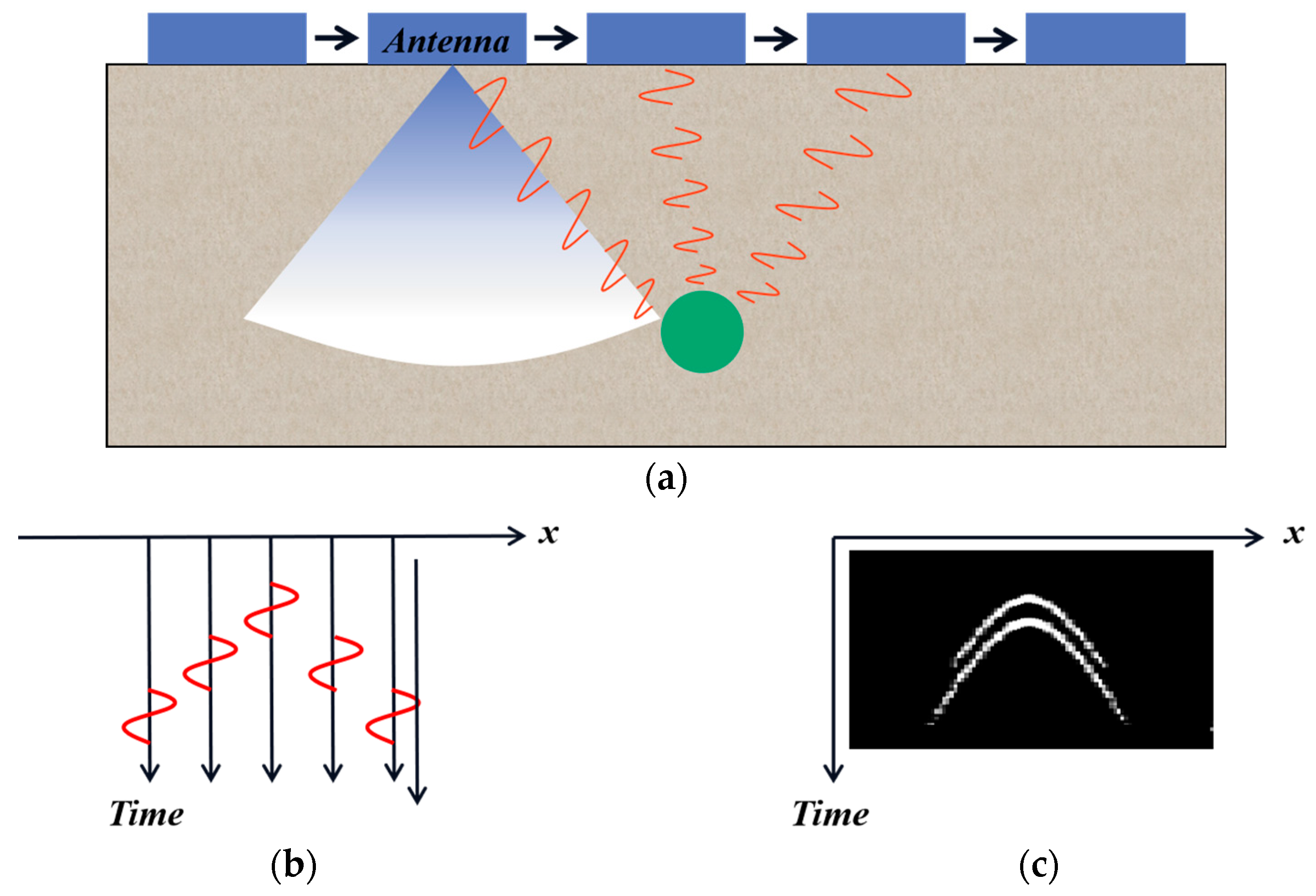
2.1. Theoretical Basis of GPR

A typical GPR system comprises three main components: a control unit (including a pulse generator, computer and related software), an antenna (comprising a pair of transmitting and receiving antennas) and a display unit [44]. The GPR transmits electromagnetic waves into the ground via the ground antenna. As electromagnetic waves propagate through different media, their electromagnetic characteristics vary depending on the dielectric properties of the materials. When the properties or types of media change, the wave will be reflected at the interface of the two media [45]. Part of the energy will be reflected, while the remaining energy will be transmitted or absorbed by the materials [42]. GPR radiates energy in a divergent elliptical cone and scans a footprint area below it, with the direction of the long axis of the elliptical cone serving as the propagation direction [46]. GPR data presented by the receiving and processing equipment is typically displayed as a radargram, which is a 2D cross-sectional image (B-scan) showing the reflections received at different depths, as shown in Figure 1. The abscissa of the B-scan is the distance, and the ordinate is the time, which reflects the distribution of the underground medium in the transect [47]. The hyperbolic features reflected in the radar profile are the most important reflection features of the target object, representing buried objects or other reflection sources. When the antenna is dragged across the surface, the return signal’s travel time from the buried object decreases to a minimum when the antenna is directly above the object, and then increases as the antenna moves away from the object, producing a characteristic hyperbola in the radar profile, as shown in Figure 2. A clear hyperbola is formed by a point or linear object with the main axis horizontal and perpendicular to the antenna’s direction of travel. Linear objects with the main axis in the antenna’s direction of travel produce linear features on the radar profile but do not produce hyperbolas. Other interception angles produce distorted hyperbolas [42].

When roots are scanned as the target object, the vertices of the hyperbola indicate the position of the root system [48], as shown in Figure 3. The electromagnetic wave emitted by the GPR antenna will first detect the upper apex of the root system, and then the electromagnetic wave will pass through the root system in the direction perpendicular to the root section and reach its lower apex, as shown in Figure 4. The black curve in Figure 4 represents the propagation of electromagnetic waves.

2.2. Theoretical Basis of gprMax Forward Modeling

gprMax is open-source software that simulates electromagnetic wave propagation using the finite-difference time-domain (FDTD) method to solve Maxwell’s equations in 3D, thus simulating the forward results of GPR [49]. Several studies have demonstrated the feasibility and accuracy of using gprMax for simulation detection in both theory and practice [50,51,52,53,54]. With gprMax, different reflected signals from various target objects in different uniform media can be simulated when they meet the propagation of radar electromagnetic wave and the position of the buried object in the underground media and the dielectric parameters of the underground media can be set. gprMax solves the problem of time-consuming and resource-intensive GPR detection.

2.3. Experimental Design

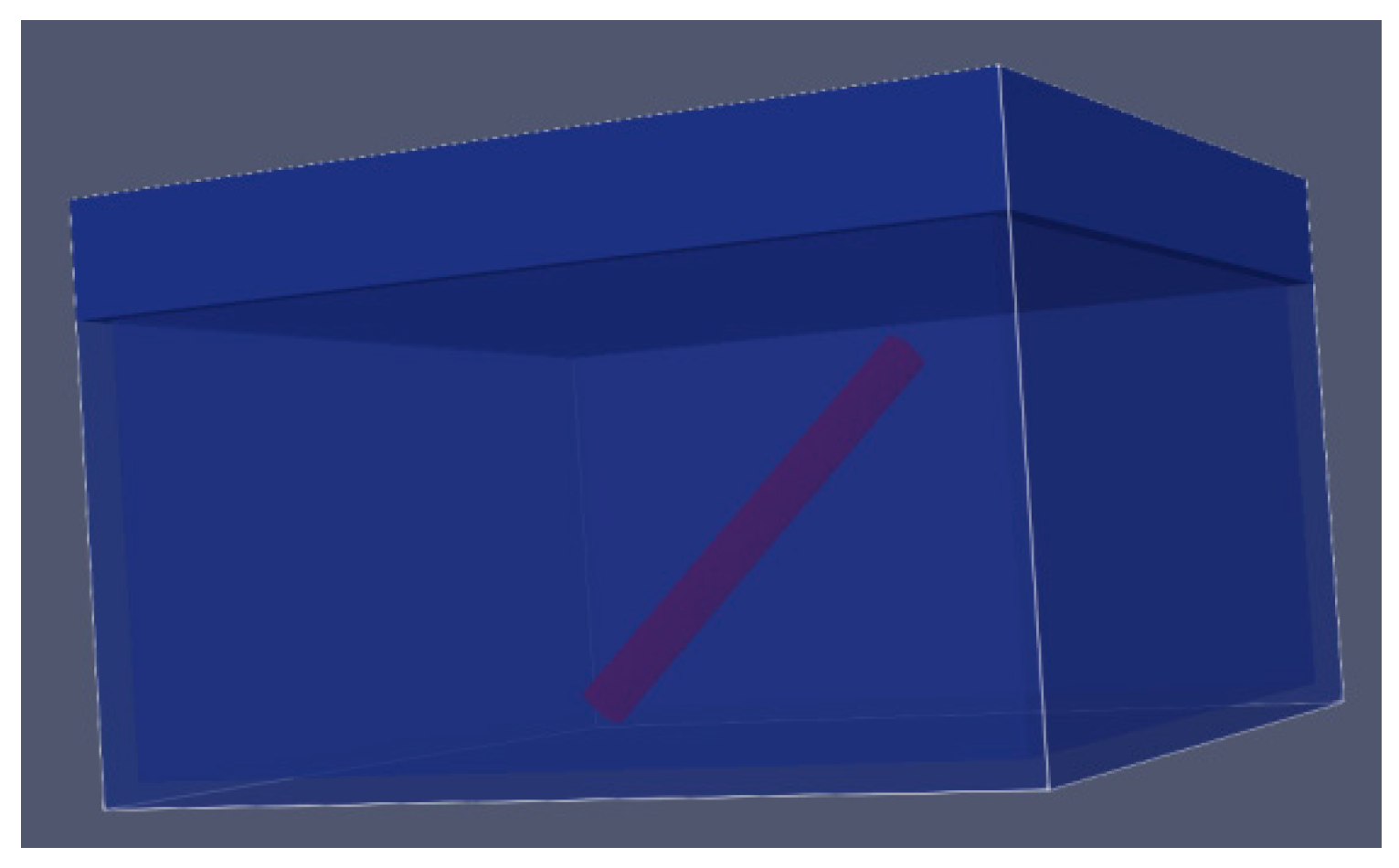
2.3.1. Tree Root Forward Simulation

In this study, the focus was on analyzing the relationship between B-scan and root diameter. Coarse roots in natural conditions are typically long and gradually narrow in diameter along their length, resembling a long cone shape. However, measuring coarse roots that are several meters long using GPR is difficult using the above method. Sawn root samples are often collected to replace coarse roots in experiments. So, short root samples with uniform thickness can be considered part of a long cone [10] and each root sample can be regarded as a cylinder.

In the experimental design, root diameters were selected as 0.01, 0.02, 0.03, 0.04, 0.05, 0.06 and 0.07 m, and the distance between adjacent root systems was 1.5 m. Previous studies on root systems by Ji et al. [55] found that more than 90% of the root systems were concentrated in the 0–50 cm soil layer of the main afforestation tree species in the river bank’s forest belt. Similarly, Yan et al. [39] found that thick roots were mainly distributed in the 0–40 cm soil layer in the Gutianshan evergreen broad-leaved forest, while Zhou et al. [56] found that the coarse roots of the Hebei poplar were mainly distributed in the 10–50 cm soil layer. Therefore, the root burial depth was set to 0.3 m, and the burial depth of all root systems was the same.

The geometric model used for simulating tree root diameter is shown in Figure 5. It depicts a vertical transect of root scanning with GPR. The lower left corner of the image represents the origin of co-ordinates. The x-axis and y-axis represent horizontal distance and vertical depth, respectively, defining a rectangular area of 10.2 m × 1.2 m. The gray area below 1 m in the vertical direction represents soil, while the white area above 1 m represents air. The green circles represent roots (7 roots in total, where R1, R2, R3, R4, R5, R6, and R7 represent the radius of roots). The transmitting and receiving antennas (red square) with a center frequency of 900 MHz move synchronously to the right along the ground from the left side of Figure 5. to complete the simulation scan. The excitation wave was set as a Ricker pulse wave with current amplitude of 1.0 A, and the step distance of the antenna was defined as 2 cm.

2.3.2. Relative Permittivity of the Tree Root and Soil Design

Guo et al. [57] measured the relative permittivity of the root and soil through field measurement in Inner Mongolia, China. They found that the relative permittivity of roots with different moisture contents ranged from 2.78 to 35.04. The relative permittivity of the soil with different forms and ingredients ranged from 2 to 30, according to the distribution of permittivity in shallow sandy layers (within 80 cm). These values of the relative permittivity of the root and soil provided a reference for the setting of the relative permittivity of the root and soil in this article. To investigate the effects of changes in the relative permittivity of the tree root and soil on the root diameter estimation model, we selected 17 different root relative permittivity values and 15 different soil relative permittivity combined values to define the model. The root relative permittivity values were increased from 3 to 35 in intervals of 2, and the soil relative permittivity values were increased from 3 to 31 in intervals of 2. The root simulation model (Figure 5) in Section 2.3.1 was set under each combination of root and soil relative permittivity, which resulted in the obtention of 240 groups of data using gprMax. Each group of data included 7 roots with a diameter from 0.01 m to 0.07 m in intervals of 0.01 cm.

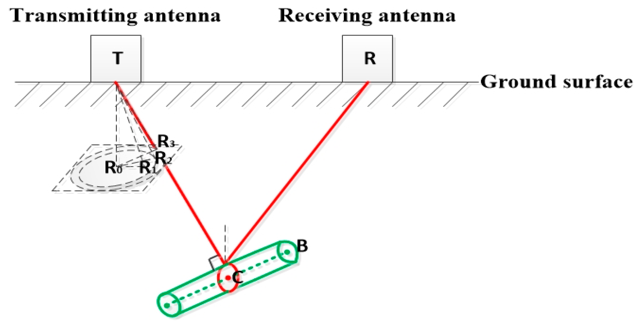
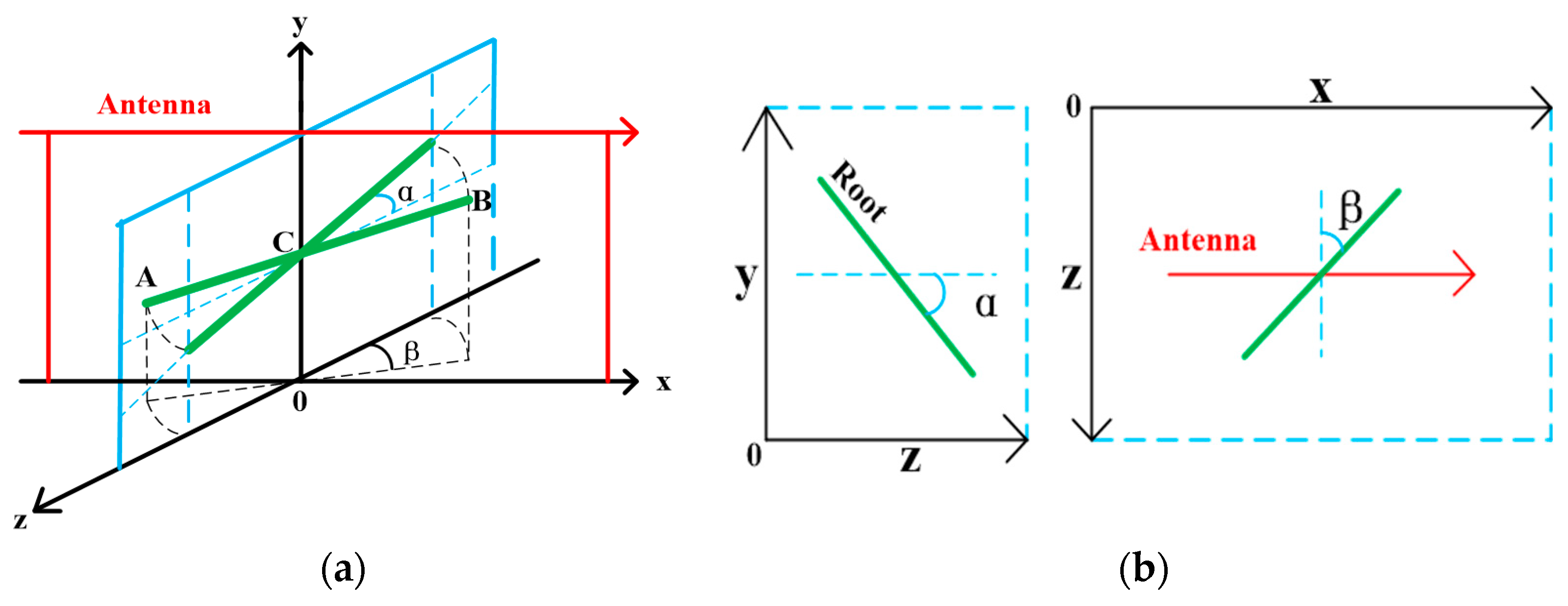
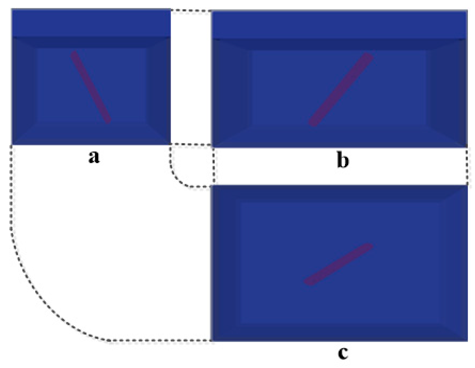
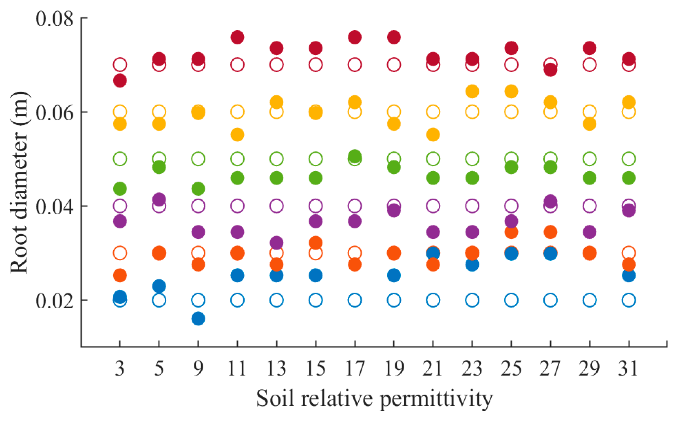
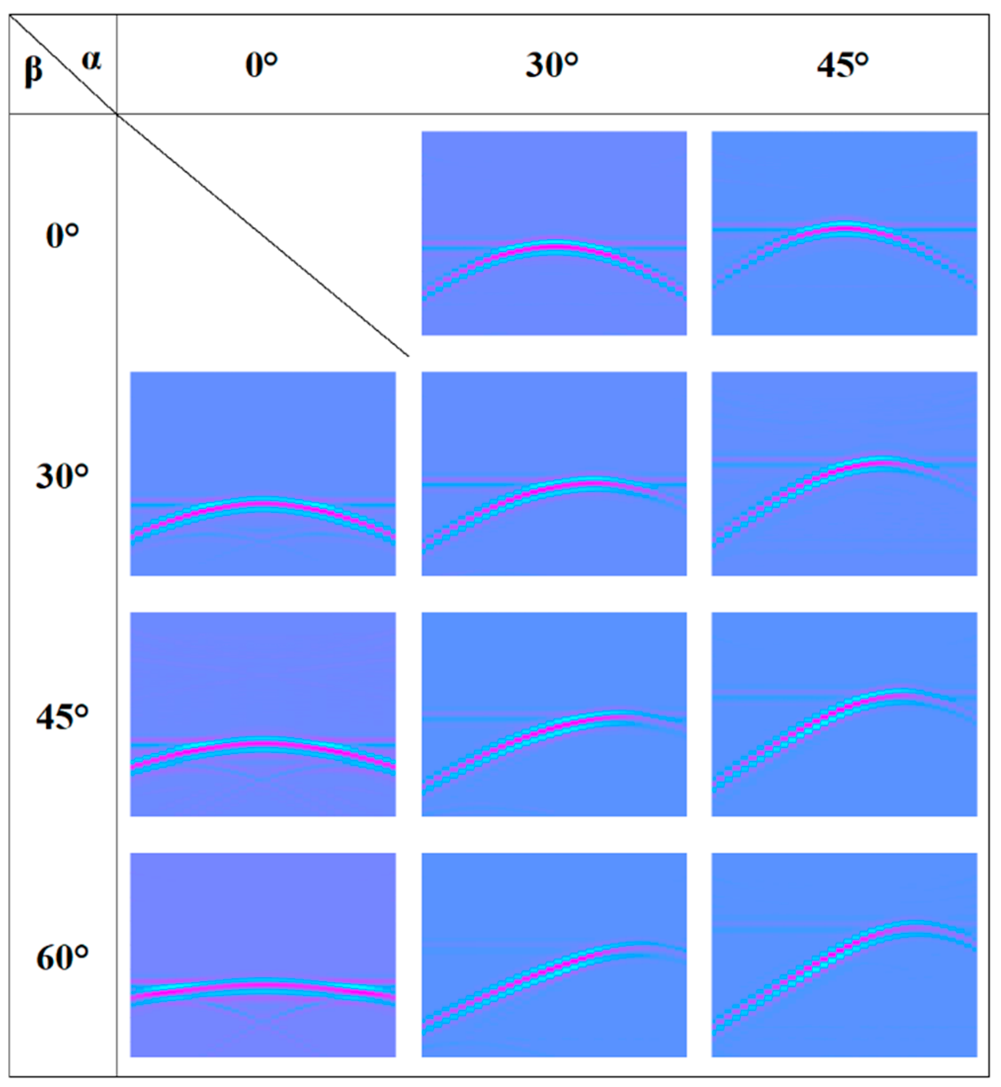
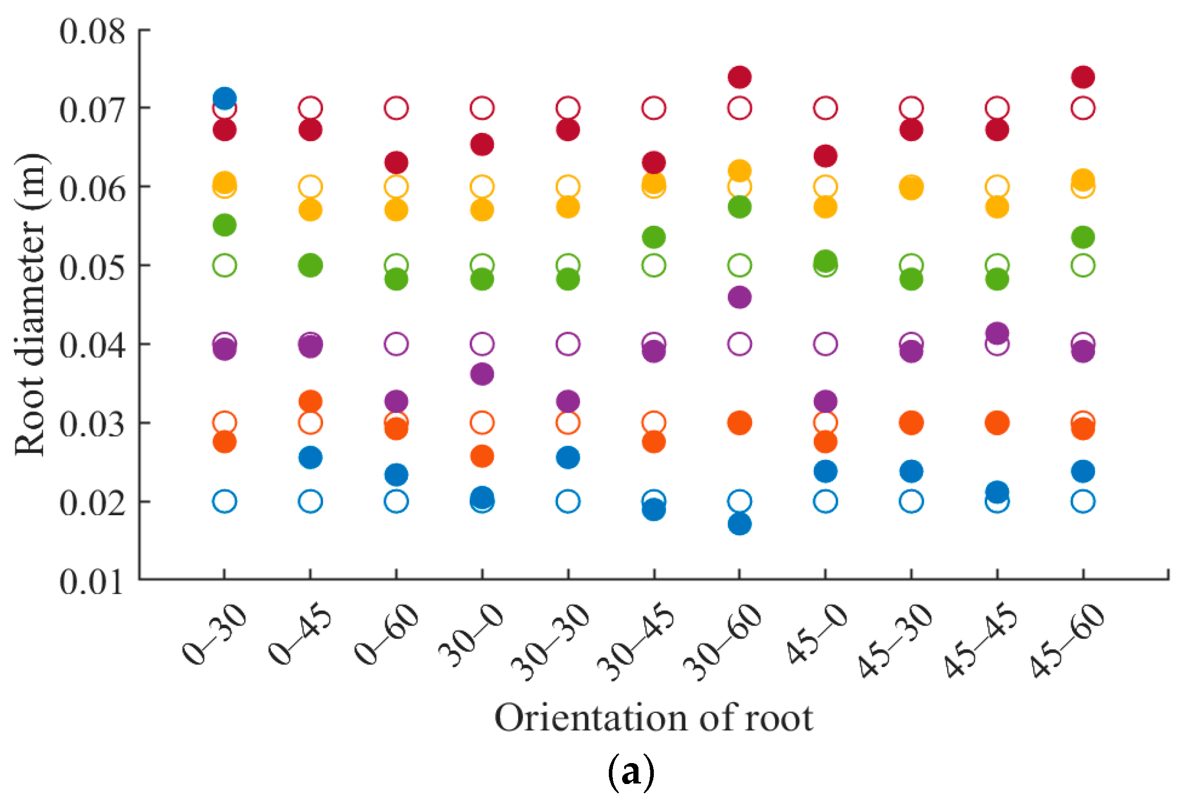
2.3.3. Tree Root Orientation Design

Root orientation is an important factor that affects root detection, specifically referring to the depolarization effect of cylindrical objects. Many researchers from previous studies have obtained models under the optimal location of the root system, where the straight line where the root system is located is perpendicular to the measuring line of antennas. To test the general applicability of the diameter estimation model presented earlier, we designed a simulation model to estimate the root diameters in different orientations. We aligned the center of the cylindrical root system to the center of the cuboid representing the scanning space and simulated the scanning of the root system with different orientations by rotating the center of the cylinder. The change in root orientation can be defined by the combined change in angles in the view side direction and the top view direction, as shown in Figure 6. We varied the angles α (0°, 30°, and 45°) and β (0°, 30°, 45°, and 60°) to define the orientations of 11 types of roots: (0°, 30°), (0°, 45°), (0°, 60°), (30°, 0°), (30°, 30°), (30°, 45°), (30°, 90°), (45°, 0°), (45°, 30°), (45°, 45°), and (45°, 60°). The schematic diagram of the model is shown in Figure 7 and Figure 8. In each model, we set the relative permittivity of the soil to 5 and the relative permittivity of the root to 10, and applied the root diameter estimation formula developed in the previous chapter. The root diameter in each model was consistent with that in the previous experiments, ranging from 0.01 m to 0.07 m.

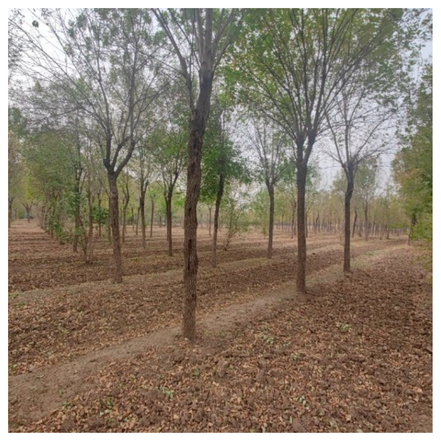
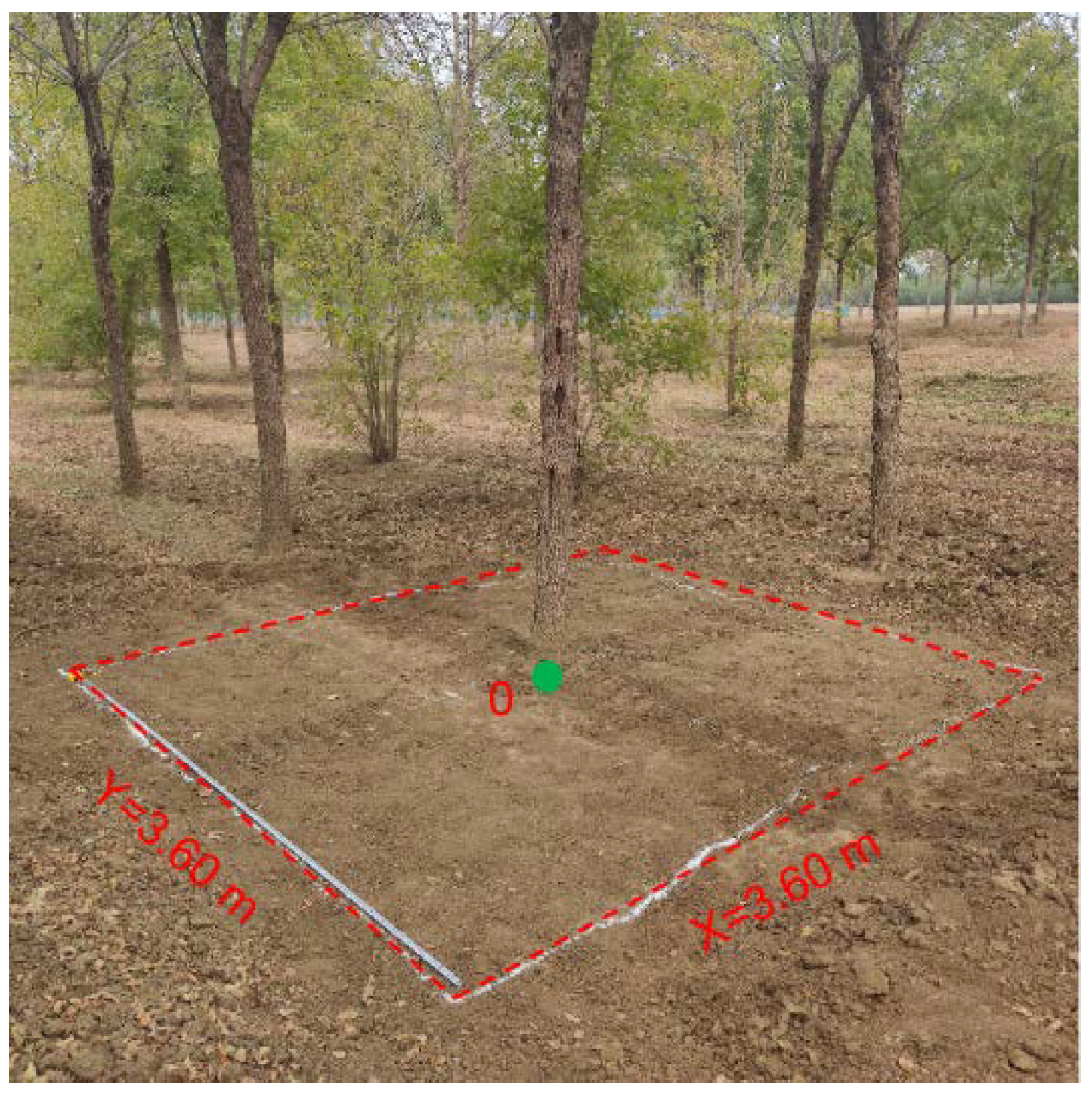
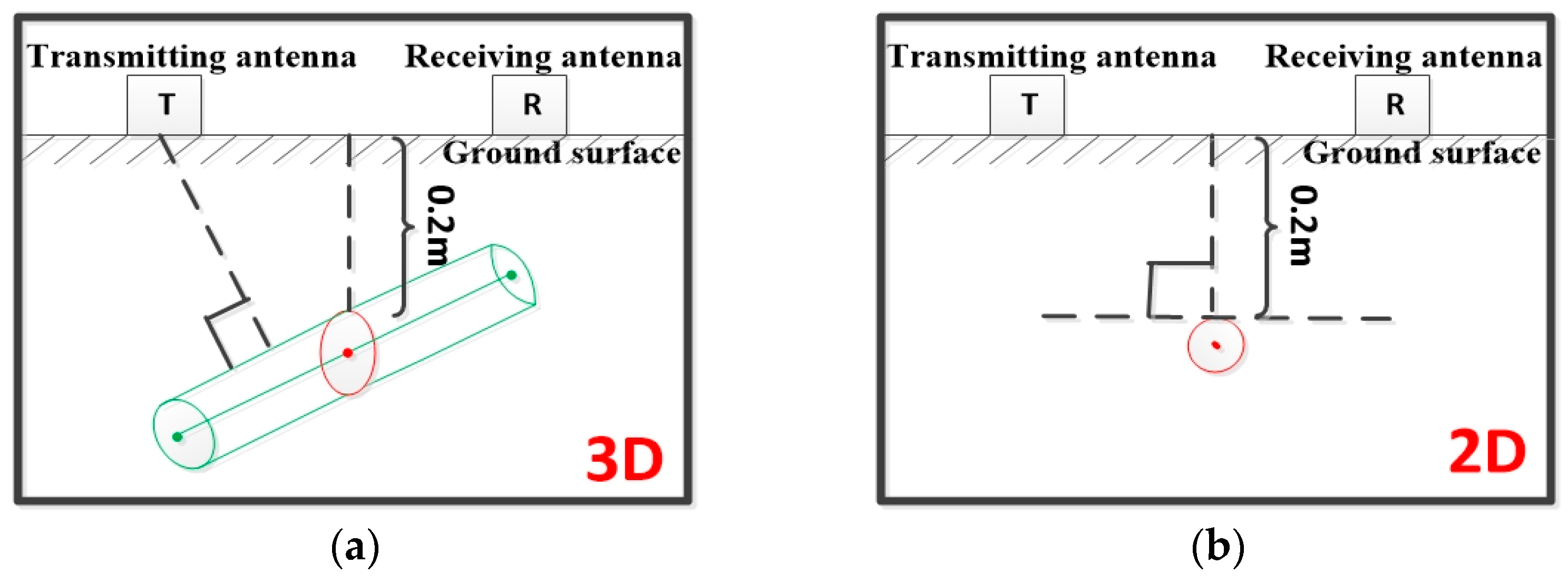
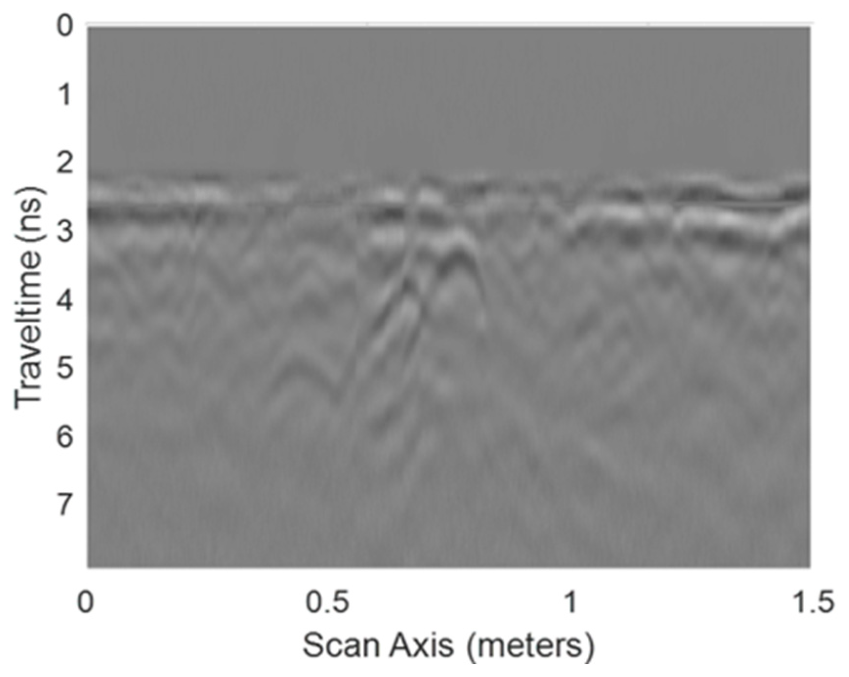
2.3.4. Field Experiment

To validate the effectiveness of the estimation model obtained from the forward simulation experiment in estimating plant roots, we conducted a field experiment in October 2022 at Xiaotangshan Nursery in Changping District, Beijing (116°24′22″ E and 40°9′38″ N), as shown in Figure 9. The study area is located in the temperate monsoon zone, with an average altitude of 40 m, and belongs to the warm temperate continental monsoon climate. The annual average precipitation is 550.3 mm and mostly occurs in July and August [58]. The soil in the study area is silty loam, with a bulk density of 1.52 g/cm³, porosity of 41.7% [59], and stable soil water content suitable for ground-penetrating radar detection.

We selected Chinese ash, a typical plant in the study area, as the research object, with a tree distance of 1.9 m × 1.9 m. We selected the root system of an ash tree with an average diameter at breast height (DBH) of 15.7 cm and centered the root collar on a rectangular area measuring 3.6 m × 3.6 m for ground-penetrating radar detection. Figure 10 shows the scene of the probe, with the north–south line representing the x-axis and the east–west line representing the y-axis. Before conducting the survey, we cleaned the litter and fallen leaves in the survey area and ensured that the ground was as flat as possible to reduce the interference of the site environment in the ground-penetrating radar scanning results.

In this study, we used TRUTM (Tree Radar Unit) from Tree Radar, Inc., Silver Spring, MD, USA, with an antenna frequency of 900 MHz to conduct ground-penetrating radar scans. We scanned along the X, Y, and parallel measurement lines, with a scanning interval of 15 cm, and obtained a total of 44 radar data profiles.

After scanning the roots with ground-penetrating radar, we sawed off the trunk 10 cm above the ground and discarded it. Then, we removed the soil to a depth of 10 cm, exposing all the tree roots. We excavated the roots of the ash tree using archaeological methods in a 2.0 m × 2.0 m range. After every 10 cm of excavation, we recorded the exposed roots and their distribution information, and sawed the root samples, particularly the coarse roots within every 10 cm depth range, which we measured. We also collected soil samples from the side walls using soil samplers to maintain the original soil structure as much as possible, taking samples from different directions several times. We repeated the process until we dug to a depth of 30 cm. After bringing the collected root and soil samples back to the laboratory, we determined the root diameter, dry and wet weight, and water content of the root and soil. We selected taproots with a symmetrical thickness and root diameter greater than 0.02 m as experimental samples. The soil samples were taken from 3 different soil layers with different water contents.

To calculate the corresponding relative permittivity of the soil with different water contents, we used the formula of Topp [60], as shown in Equation (1):

$${\epsilon }_{\mathrm{r}}=3.03+9.3{\theta }_{\mathrm{w}}+146.0{\theta }_{\mathrm{w}}{}^2-76.7{\theta }_{\mathrm{w}}{}^3$$

(1)

where ε_r is the relative permittivity of the soil, and θ_w is the water content (%) of soil.

The root system can be considered a four-phase mixture of root dry matter, pores, bound water, and free water. We used the relative permittivity and volume percentage of each component to estimate the relative permittivity of the root mixture [61] (Paz et al., 2011), as shown in Equation (2):

$${\epsilon }_{\mathrm{m}}^{\prime }{}^{\beta }={\theta }_{\mathrm{f}\omega }\times {\epsilon }_{\mathrm{f}\omega }^{\prime }{}^{\beta }+{\theta }_{\alpha }\times {\epsilon }_{\alpha }^{\prime }{}^{\beta }+{\theta }_{\mathrm{s}}\times {\epsilon }_{\mathrm{s}}^{\prime }{}^{\beta }$$

(2)

where ε′ is the relative permittivity and θ is the percentage of volume. The subscripts m, fω, α, and s represent the percentage by volume of root mixture, free water, air, root dry matter and bound water mixture, respectively. β is the geometric factor. ${\epsilon }_{\mathrm{f}\omega }^{\prime }$, ${\epsilon }_{\alpha }^{\prime }$, ${\epsilon }_{\mathrm{s}}^{\prime }$ and β are equal to 80, 1, 10 and 0.36, respectively [61]. After root moisture content exceeded the fiber saturation point, the proportion of bound water to dry weight was about 30% [62]. Therefore, we calculated the mass of free water and bound water based on the dry and wet weight of roots measured. The density of free water and bound water was 1 g/cm³, and the density of root dry matter was 1.53 g/cm³ [61]. Based on this, we calculated the volume of the mixture of free water, dry matter, and bound water. The total volume of the root sample was approximately the volume of a cylinder, so the air volume was the total volume minus the sum of the mixture volumes of free water, dry matter, and bound water. The volume fraction of each component was substituted into Equation (2) to calculate the relative permittivity of roots with different diameters and water contents.

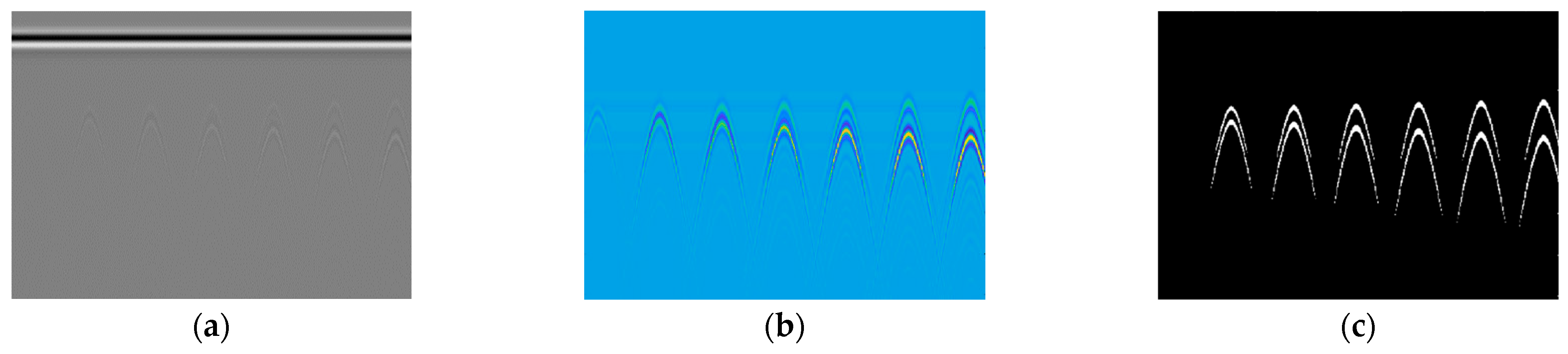
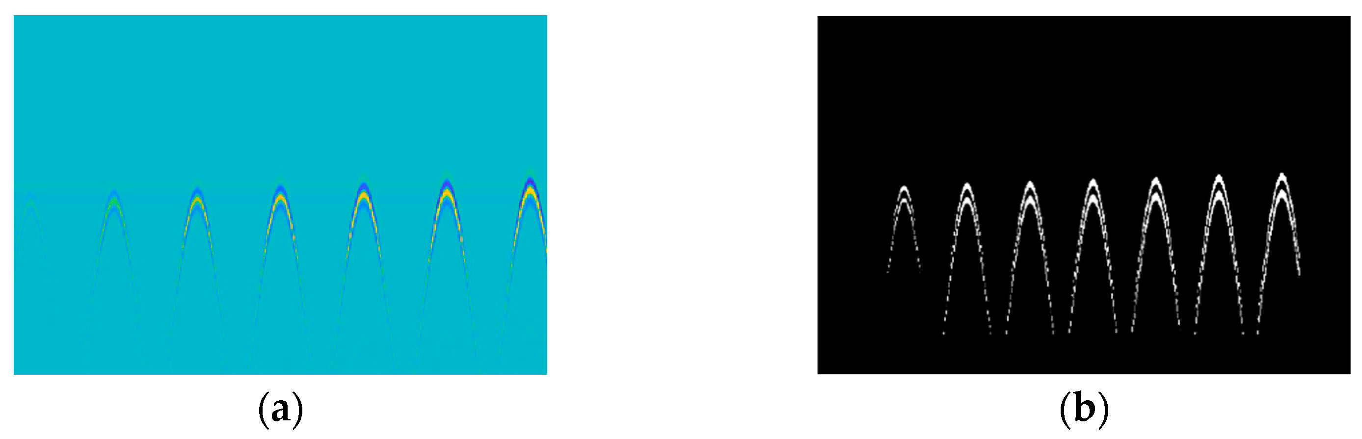
2.4. Data Preprocessing

The scan map obtained via GPR is not convenient for the direct observation of the hyperbola, so some processing of the scan result is necessary. Firstly, the gray scale of the B-scan is processed to make the contour of the hyperbola clearer. However, due to the existence of background clutter, the hyperbola features become blurred in the radar profile. The clutter mainly comes from the direct surface waves generated by the interaction between the radar antenna and the ground, so it is necessary to remove the direct waves in the B-scan diagram. The HSV color space can well-separate color information and brightness information and place them in different channels, reducing the influence of light on specific color recognition [62]. This is because the HSV color space separates the color information from the brightness information, allowing for more robust color analysis and recognition under varying lighting conditions. H represents the color, S represents the depth of the color, and V represents the shade of the color. In order to extract a clear hyperbola, according to the color characteristics in the data after the direct wave is removed, the hyperbola that can clearly reflect plant roots is extracted by setting the value of HSV.

3. Results

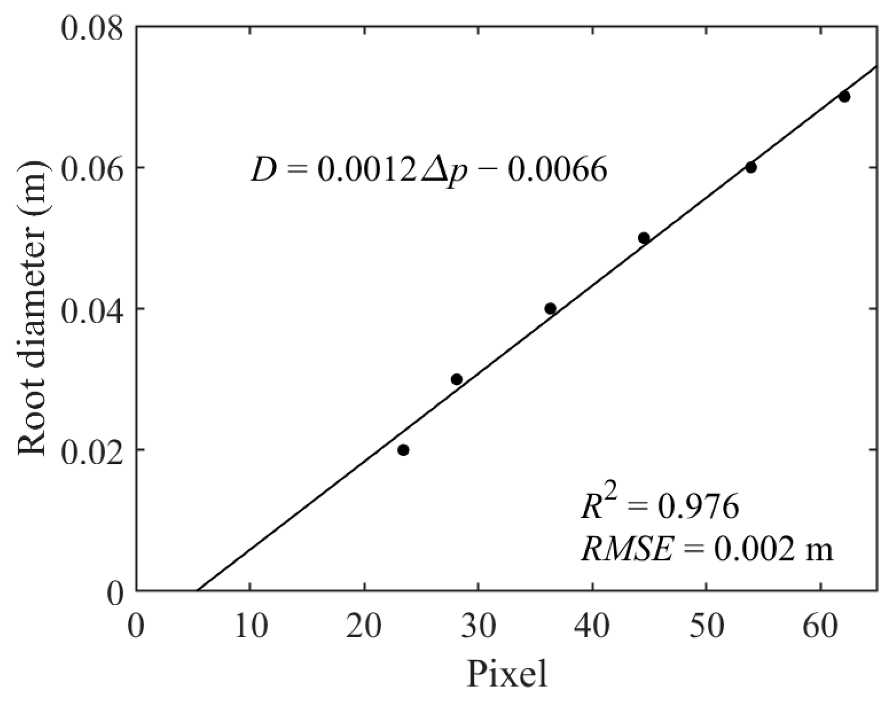
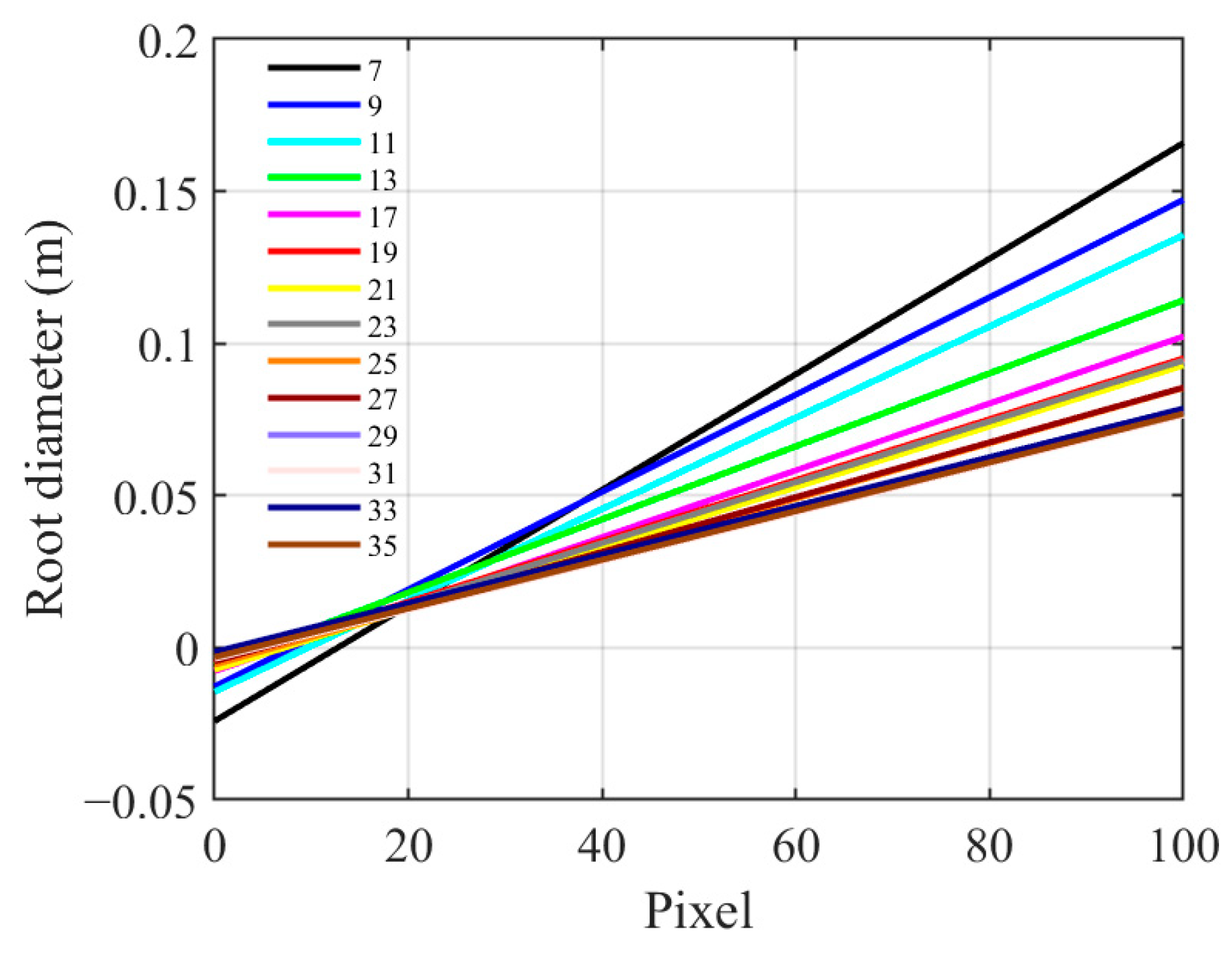
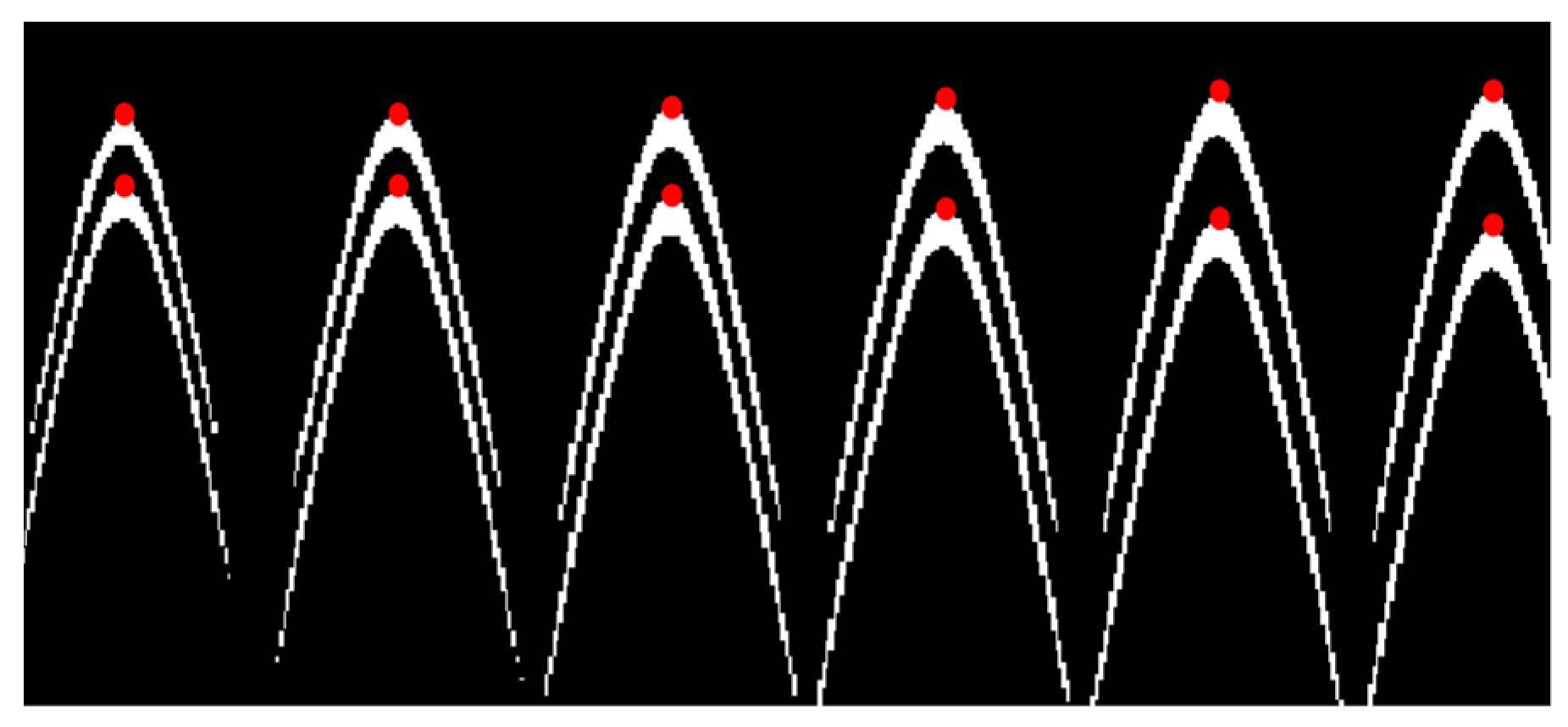
3.1. Relationship between Root Diameter and Pixel Distance

Briefly, there were 240 different combinations of root and soil relative permittivity. Each group of data contained the scanning results of seven roots with diameters ranging from 0.01 m to 0.07 m. The analysis of the root samples in the simulation indicated a definite positive linear relationship between the root diameter and the pixel distance between the vertices of two hyperbola (∆p) obtained through it.

Taking the data set with a relative permittivity of 15 for roots and of 5 for soil as an example, Figure 11 shows the scanning results of different processing. In Figure 11c, the ordinate of the B-scan showing the scanning results represents time, and the upper and lower vertices of the two hyperbolas also represent time, corresponding to the moment when the electromagnetic wave enters and exits the tree root (T₁ and T₂, respectively). Additionally, the vertex of the upper hyperbola corresponds to the upper vertex of the root system, and the vertex of the lower hyperbola corresponds to the lower vertex of the root system. It can be observed that the distance between the upper and lower hyperbolas increases as the diameter of the root increases, which represents the time interval (∆T) for the electromagnetic wave to pass through the root. This is because the propagation distance of electromagnetic waves at the root increases with size, resulting in a longer time between two reflected waves [63]. T₁ and T₂ can be represented by pixel values p₁ and p₂ in the picture after threshold processing, while ∆T can be represented by ∆p. p₁ is the pixel value of the vertex of the first hyperbola, and p₂ is the pixel value of the second hyperbola. Hence, ∆T is proportional to ∆p, and ∆p also changes with the changes in the root diameter. Additionally, compared to ∆T, the value of ∆p is easier to obtain via the method of threshold extraction.

Furthermore, the identification effect of the upper and lower boundaries of roots with a diameter of 0.01 m is vaguer than that of roots with other diameters. The upper and lower boundaries of roots with a diameter of 0.01 m cannot be identified in the result of HSV component extraction, indicating that the upper and lower surfaces of roots smaller than 0.01 m are difficult to reflect in the entire electromagnetic wave propagation process.

This is because the propagation process of the electromagnetic wave in the coarse root cannot be ignored. The coarse roots have larger diameters as the propagation distance of the electromagnetic wave and ∆T between the electromagnetic wave entering (the apex of the first hyperbola) and exiting (the apex of the second hyperbola) through the roots is well-represented in the obtained B-scan, resulting in two hyperbolas with obvious distances in the B-scan. For some fine roots, the propagation distance of electromagnetic waves in the soil medium is much greater than the propagation distance of electromagnetic waves in the root system, and the hyperbola is difficult to reflect in the simulation results. Therefore, such fine roots cannot be detected via GPR and are not included in the study. The ∆p between the upper and lower vertices of the hyperbola corresponding to each root was extracted from the simulation results, corresponding to root diameters of 0.02, 0.03, 0.04, 0.05, 0.06, and 0.07 m, as shown in Figure 12.

When the GPR data contained only a few root samples, it was challenging to create a reliable complex regression model. In such cases, a simple linear regression model was more feasible. We fitted a linear regression model to these data to establish their relationship with the true diameter value, with a determination coefficient (R²) of 0.976 and a root mean square error (RMSE) of 0.002 m, as is shown in Figure 13. The model is shown in Equation (3):

$$D=0.0012\Delta p-0.0066$$

(3)

where ∆p is the pixel distance between the upper and lower hyperbola in B-scan and D is the estimated data of the root diameter.

Similar scanning results also appeared in the scanning data of 212 groups obtained when the relative permittivity of roots was 7, 9, 11, etc. Similarly, we obtained 212 linear fitting results of ∆p and root diameter under different combinations of root relative permittivity and soil relative permittivity, which can be used as root diameter estimation models (Model 1). However, when the relative dielectric constant of the roots was three and five, the obtained scanning results could not observe the change process of the distance between the two vertices of the hyperbola increasing with the increase of the diameter of the roots, as shown in Figure 14.

The relative permittivity plays a vital role in the propagation of the wave speed. The expression of the electromagnetic wave speed is shown in Equation (4):

$$v=\frac{c}{\sqrt{{\epsilon }_r}}$$

(4)

where v is the propagation speed of the electromagnetic wave in a vacuum, c is the same as the speed of light and ε_r is the relative permittivity of the propagation medium.

Therefore, the speed of the electromagnetic wave passing through tree roots is related to the relative permittivity of tree roots. When the relative permittivity of plant roots is too small, the speed of the electromagnetic wave will be very fast, and the ∆T of electromagnetic wave passing through the roots will be very short. As a result, the difference between the ∆T required to pass through different roots with their diameters increasing in an interval of 1 cm is almost negligible. In the B-scan, it is difficult to clearly display the increasing distance between the upper and lower vertices of the hyperbola corresponding to the increasing diameters of the roots and to apply these ∆p changes to develop the diameter estimation model. Thus, the data obtained for the roots with relative permittivity values of 3 and 5 are also not included in the following study.

To verify the accuracy of the estimation models obtained in this study and avoid any chance factors, we calculated the diameters of 1272 effective roots in this experiment using the estimation models obtained and the ∆p of the corresponding hyperbolas in the B-scan. The RMSE and R² values were obtained as 0.0023 m and 0.9816, respectively. The small value of RMSE is an indicator of the model’s excellent estimation effect. Additionally, the R² value, which is close to 1, suggests a high degree of correlation. As shown in Figure 15, when the relative permittivity of the roots was 7, we compared the estimated values of roots with diameters of 0.02–0.07 m with the actual values under different soil relative permittivity values. It is shown that the coincidence degree between the estimated value of model and the actual value is high, which represents a good estimation effect.

The experimental results confirm the feasibility of using B-scan results to estimate the diameter of underground roots. However, due to the complexity and uncertainty of the root growth environment under actual conditions, the results obtained via the current GPR in field detection may deviate from forward modeling results and reveal inaccurate estimation results. In such cases, image processing technology can be used to filter the original data and achieve a more accurate estimation of the diameter of the underground root systems of trees.

3.2. Effects of Relative Permittivity of the Tree Root and Soil on Modeling Tree Root Diameter

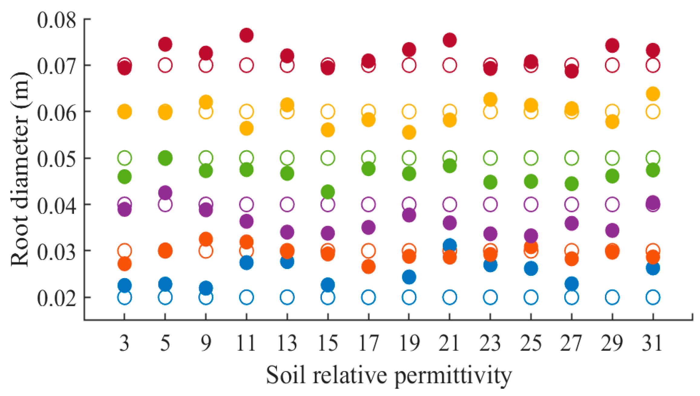
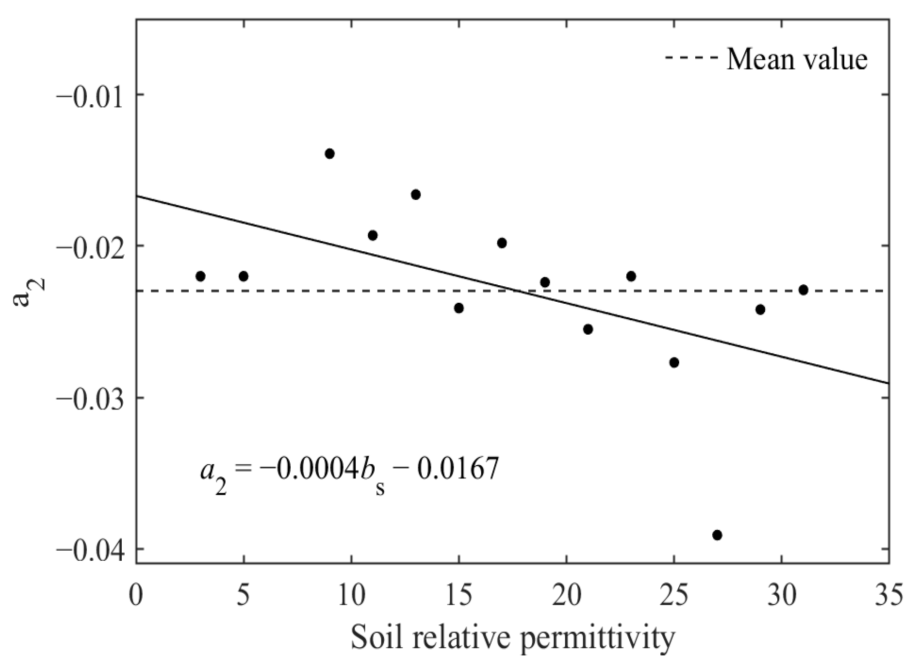
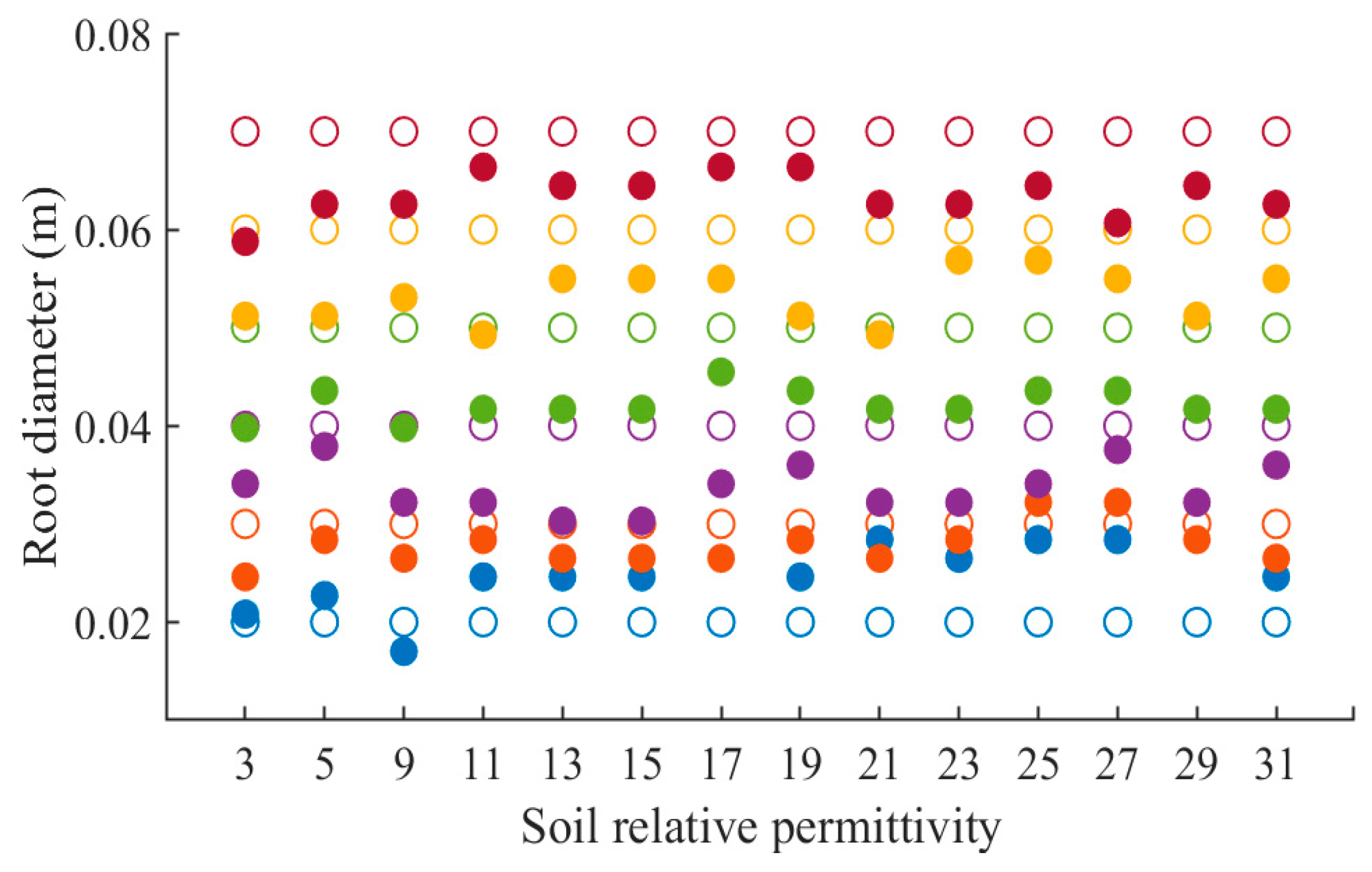
3.2.1. Relationship between Soil Relative Permittivity and Root Diameter Estimation Equation

The simulation results presented above demonstrate that the 212 root diameter estimation models obtained can be practically used for prediction if the relative permittivity of the soil and root is known. When selecting the fitting model, it is important to note that the accuracy of the prediction increases with the proximity of the measured values of the soil and root relative permittivity to the actual environment.

In the case of roots with a relative permittivity of 7, 14 root estimation models were obtained by fitting the diameters of 6 different roots and their corresponding ∆p under different soil conditions with varying relative permittivity. Figure 16 illustrates the estimation models obtained under different soil relative permittivity conditions with the root relative permittivity of 7. These results showed that soil relative permittivity had little effect on the diameter estimation model. It was observed that the slope and intercept of these estimation models fluctuated slightly over a range and could be approximated to the same linear equation. The slope and intercept of the 14 estimation models were fitted with the relative permittivity of soil, respectively, and the results are shown in Figure 17 and Figure 18. It was found that the values of these slopes are all very similar and that they can be viewed as fluctuating around a straight line, which means the slope of the diameter estimation models does not change with the change in soil relative permittivity. On the other hand, the value of the intercept would vary slightly with the slope fluctuations in the model.

For further research, we developed a new diameter estimation model (Model 2) by taking the average values of the slopes and intercepts obtained using fourteen linear models for a root relative permittivity of 7, as shown in Equation (5):

$$D=0.0020\Delta p-0.0230$$

(5)

We estimated the root diameter again, and the estimated values of roots with diameters of 0.02~0.07 m were compared with the actual values under different soil relative permittivity conditions when the relative permittivity of roots was 7, as shown in Figure 19. The residuals of the estimated results of diameter obtained from the original model and the new model are shown in Figure 20. The residual span of the prediction results of the previous model (Model 1) is about 0.0170 m, and the residual span of the new model (Model 2) is about 0.0177 m, indicating that the overall distribution range of the predicted residual of the original model is small, that the overall distribution range of the new model is slightly larger than that of the original model, and that the stability of the prediction performance of the model decreases. The range of the upper quartile (Q75%) and lower quartile (Q25%) of the original model is about [−0.0031 m, 0.0026 m], and the corresponding value of the new model is about [−0.0032 m, 0.0035 m], which indicates that the original model has a more concentrated residual distribution. However, there was an outlier in the old model that is not present in the new one. Moreover, the median of the residual distribution of the new model is −0.0002 m, which is closer to 0 than the median of the previous model, −0.0006 m.

In summary, the estimation error of the new model is greater than that of the previous model. However, the estimation results are better, making the model more suitable for rough estimations. Thus, changes in soil relative permittivity should not affect the linear estimation model. By using the method of finding the average value, we were able to obtain 15 fitting expressions that corresponded to the different relative permittivity values of roots. Using these expressions, we re-estimated the diameters of 1272 roots in our experiment. The resulting RMSE and R² values were 0.0029 m and 0.9708, respectively.

In this experiment, although different groups of data had different soil relative permittivity values, they all had the same root relative permittivity value. According to the expression of electromagnetic wave velocity (Equation (4)), the electromagnetic wave velocity was only related to the relative permittivity of the root. As a result, the velocity electromagnetic wave traveling through the roots in different groups of data was the same. Hence, ∆T was determined by the size of the root diameter and when the electromagnetic wave traveled through a root with the same diameter in different groups of data was unchanged, ∆T was unchanged. As a result, ∆p would not change. Therefore, the diameter estimation model was only affected by the relative permittivity of the roots, not the relative permittivity of the soil.

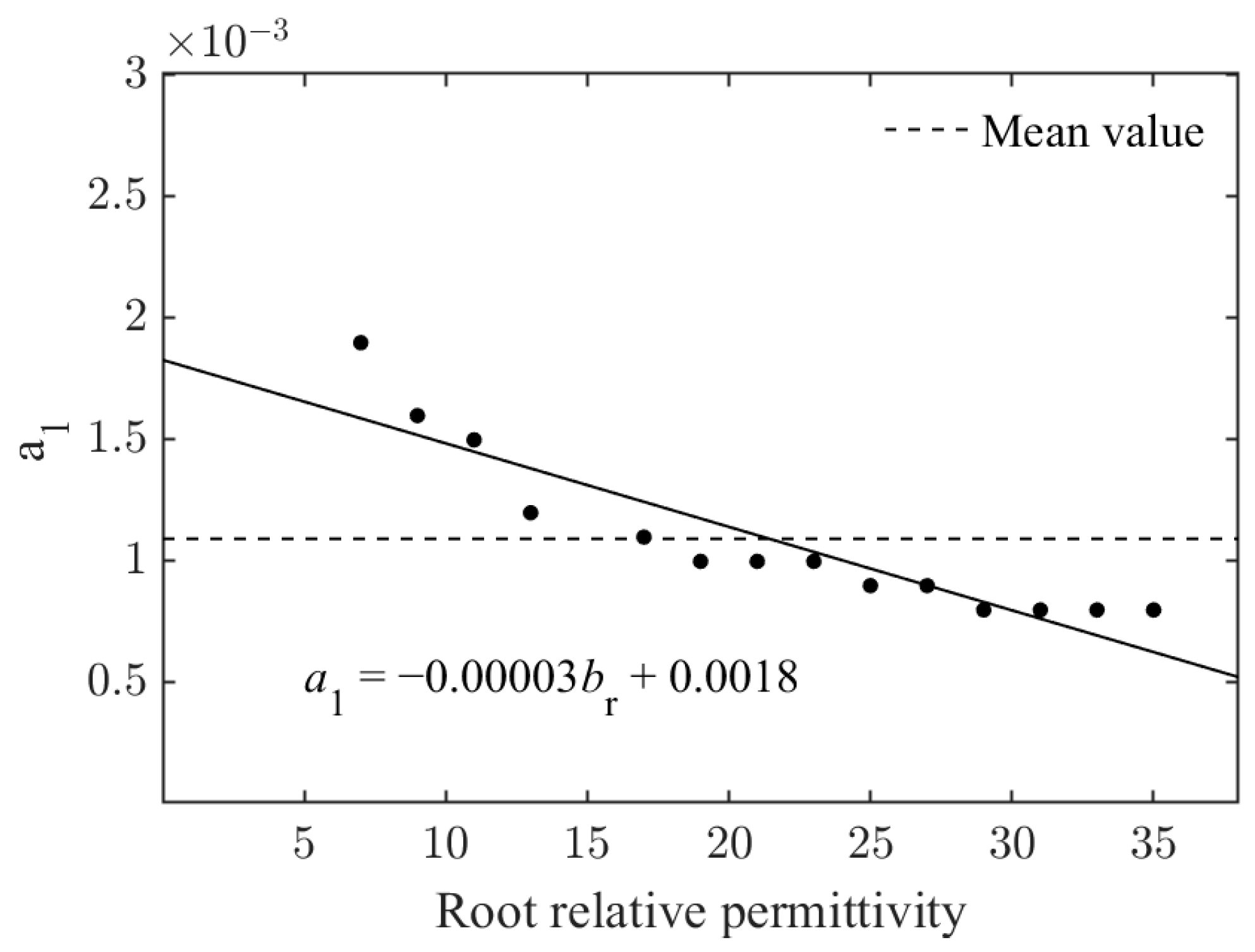
3.2.2. Relationship between Relative Permittivity of Root System and Root Diameter Estimation Equation

To explore how the relative permittivity of roots affects the diameter estimation model, we selected the data set with a soil relative permittivity of 15 for analysis from 212 groups of data. Under this condition, 14 estimation models were obtained under different root relative permittivity values, as shown in Figure 21. When the soil relative permittivity remained unchanged, but the root relative permittivity was changed, the diameter estimation models obtained by diameter and ∆p fitting were different. Moreover, with an increase in root relative permittivity, the slope of estimation models gradually decreased, and the intercept gradually increased. The slope and intercept of the 14 estimation models were linearly fitted with the relative permittivity of the root, and the results are shown in Figure 22 and Figure 23.

It is evident that both the slope and intercept change regularly with an increase in the relative permittivity of roots. The fitting equations of the slope and intercept pertaining to the relative permittivity of roots were obtained, which can estimate the slope and intercept in diameter estimation models under different root relative permittivity conditions. The slope and intercept estimation equations are shown in Equations (6) and (7):

$$a_1=-0.00003b_r+0.0018$$

(6)

$$a_2=0.0006b_r-0.0191$$

(7)

where b_r is the relative permittivity of root, a₁ is the slope and a₂ is the intercept in the root diameter estimation equation to be confirmed.

It is hypothesized that a fitting equation for estimating the diameter of roots in relation to soil relative permittivity can be obtained by observing the corresponding estimation models for various roots, under fixed soil relative permittivity. The slope and intercept coefficients of these equations fluctuate smoothly within a certain range. To estimate the slope and intercept in the diameter estimation model at a fixed relative permittivity of soil, 15 fitting equations were derived. The average values of the two coefficients of these equations were then calculated, and the resulting values were used to obtain the new slope and intercept estimation equations. These equations are shown in Equations (8) and (9).

$$a_1=-0.00003b_r+0.0018$$

(8)

$$a_2=0.0005b_r-0.0193$$

(9)

We developed another diameter estimation model (Model 3) for a root relative permittivity of 7 using Equations (8) and (9) above, as shown in Equation (10):

$$D=0.0016\Delta p-0.0157$$

(10)

We used two models to calculate the slope and intercept of the diameter estimation model for a root relative permittivity of 7. The confirmed diameter estimation model was then used to estimate root diameter, and the estimated values ranging from 0.02 to 0.07 m were compared with actual values for different soil relative permittivity levels. This comparison is shown in Figure 24. The residual distribution of the three models is presented in Figure 25.

The latest model (Model 3) predicts a residual span of about 0.0158 m, with the upper (Q75%) and lower (Q25%) quartiles of the residual distribution ranging from −0.0078 m to −0.0023 m, and a median of −0.0052 m. While the latest model has the smallest residual span and upper and lower quartile distribution span compared to the previous two models, the median deviates from 0 the most, and there are two outliers. Therefore, the overall distribution range of the latest model residuals is smaller and more concentrated, indicating that the prediction stability of the model is higher, but the estimation error is much higher than that of the previous two models. Although the estimation effect of the improved model is not as good as that of the previous two models, it still represents a useful guideline for rough diameter estimation as a universal method. By employing a method that calculates the slope and intercept, we were able to derive 15 fitting expressions that corresponded to the different relative permittivity values of roots. We applied this method to estimate the diameters of 1272 roots in our experiment, resulting in a RMSE of 0.0047 m and an R² value of 0.9290.

These experiments showed that the diameter estimation equation is affected by the relative permittivity of the root, which can be explained by the velocity expression of the electromagnetic wave (Equation (4)). The electromagnetic wave propagated through the root, and its propagation speed was related to the relative permittivity of the root. With the change in the relative permittivity of the root, the propagation velocity of electromagnetic wave also changes. As a result, the ∆T of the electromagnetic wave in root with the same diameter changed in different groups of data, and then the ∆p also changed, thus affecting the diameter estimation model. At the same time, the diameter estimation model could be established under the condition of known relative permittivity of roots.

3.3. Feasibility of Applying Diameter Estimation Model to Tree Roots of Different Orientations

The electromagnetic wave emitted by the GPR is spherical. The ordinate of the hyperbola in the B-scan diagram reflects the propagation time of the GPR’s receiving end to a certain detection point of the target object. In the same homogeneous medium, electromagnetic waves propagate at the same speed. Therefore, the shorter the propagation time, the shorter the propagation distance between the GPR receiver and the target object’s detection point. Thus, the vertex of the hyperbola in the B-scan figure corresponds to the detection point with the shortest propagation distance from the GPR receiver to the target object. When the root system is used as the target object to be detected, the hyperbola vertices in the B-scan graph obtained during scanning correspond to the shortest distance between the GPR receiving end and the root system. That is, the electromagnetic wave does not simply propagate in the vertical plane where the antenna moves, and the B-scan does not reflect the propagation of electromagnetic wave in the profile where the antenna moves (Figure 26b), but the propagation of the electromagnetic wave to the underground surroundings at every point when the antenna moves (Figure 26a). Therefore, the shortest distance is the space distance between the line where the antenna moves and the line where the root is located. According to the propagation properties of electromagnetic waves, the vertices of the two hyperbolas always correspond to the upper and lower boundaries of the root diameter, regardless of the root’s spatial orientation.

In the experiment aimed at estimating the diameter of roots in different orientations, we simulated 66 root systems, each with unique growth orientations and diameters. The simulations of 11 root orientations are shown in Figure 27. Additionally, we obtained the GPR scanning results of roots with the same diameter under different orientations, as shown in Figure 28.

According to the simulation results, we can conclude that the influence of the angle change in the side view direction on the detection results of GPR is smaller than that in the top view direction. With the angle change in the top view direction (greater than 0 degrees), the angle change in the side view direction also leads to different degrees of change in the simulation results. When the angle of the top view direction is larger, the root system is closer to being parallel to the detection line of the antenna, and the simulation result is closer to an approximately straight-line hyperbola. Thus, GPR can express roots growing at different angles. We then discuss the application of the diameter estimation model to the diameter of the root with different orientations.

Two diameter estimation models, Model 2 (Equation (5)) and Model 3 (Equation (10)), were used to estimate the diameter of roots in 11 different orientations in soil with a relative permittivity of 17. The models were based on a root relative permittivity of 7. The estimated root diameters of 0.02–0.07 m were compared to the actual values, and the results are plotted in Figure 29. Figure 29a shows the estimated effect of Model 2, while Figure 29b shows the estimated effect of Model 3. The results indicated that the error in estimation results using Model 3 increased with the increasing diameter. However, Model 2 had a good estimation effect even for roots with different orientations.

Figure 30 displays the residual difference of diameter estimation results obtained using Models 2 and 3. The residual span of prediction results obtained via Model 2 using Equation (5) was about 0.0147 m, while the residual span of Model 3 calculated using Equations (8) and (9) was about 0.0191 m. This indicates that the overall distribution range of residuals predicted by Model 2 is smaller, while the overall distribution range of residuals predicted by Model 3 is larger, decreasing the stability of the predictive performance of the model. The range of the upper quartile (Q75%) and lower quartile (Q25%) of the residual distribution in Model 2 was approximately [−0.0020 m, 0.0028 m], and the corresponding value of Model 3 was approximately [−0.0016 m, 0.0088 m]. This indicates that the residual distribution in Model 2 is more concentrated. Furthermore, the median of residual distribution of Model 2 was −0.0009 m, which is closer to 0 than the median of Model 3, which was −0.0047 m. Generally, the error of the estimated data obtained using Model 3 was larger than that obtained using Model 2, and the estimation effect of Model 2 was better. Based on the statistical results, Model 2 had an R² value of 0.8058, while Model 3 had an R² value of 0.5625. Additionally, the corresponding RMSE values for Model 2 and Model 3 were found to be 0.0072 m and 0.0089 m, respectively.

The results indicate that when the root orientation is deflected, the estimation error is significantly greater compared to that when the root is placed horizontally. This suggests that the angle between the measuring line and root orientation can affect the diameter estimation model. This is due to the narrow width of the hyperbola reflected from the root in the GPR profile when the included angle is 90°. However, when the included angle is less than 90°, the hyperbola becomes wider and relatively flat [31]. In GPR detection, under optimal detection conditions, where α is equal to 0° and β is equal to 0°, the estimation error is usually smaller than that under other conditions. Nonetheless, the estimation model can still provide a rough estimation of coarse root diameter within a certain error range.

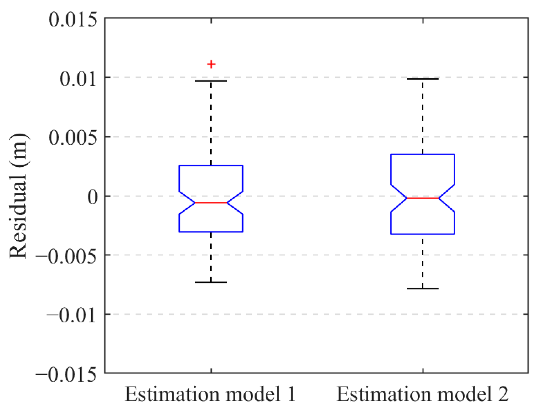
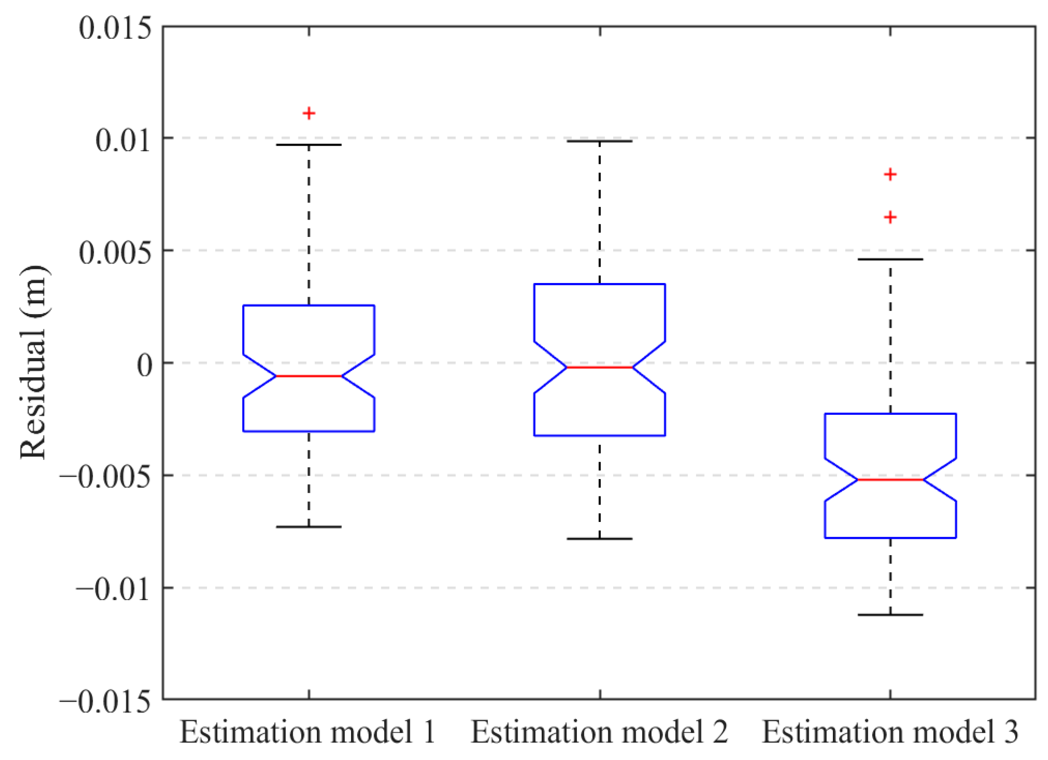
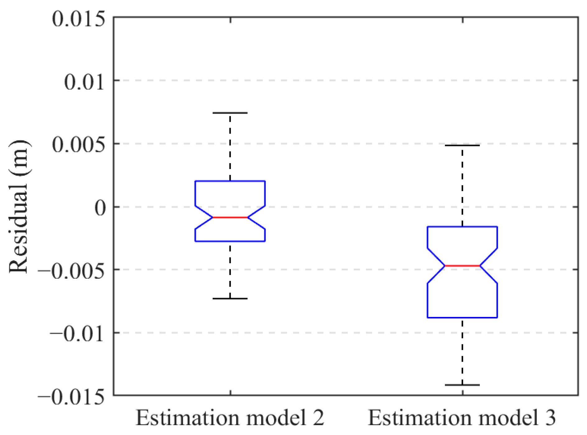
3.4. Feasibility of Applying Diameter Estimation Model to the Field Tree Root

In total, 44 scanning images of transects were obtained according to the square grid scanning scheme. The processed scanning result is displayed in Figure 31. From all the sawn root samples, eight qualified root samples were chosen as experimental samples, and their relative permittivity, along with the relative permittivity of three soil samples at different depths, which were calculated, respectively using Equations (1) and (2).

Table 1. Electromagnetic properties of media.

Media	Number of Samples			Deep (cm)	Relative Permittivity
soil	1			0–10	4.58
	2			10–20	5.70
	3			20–30	6.03
root		Diameter (cm)	Water content
	1	2.37	65%	0–10	5.38
	2	2.29	72%	0–10	5.63
	3	3.08	101%	10–20	13.59
	4	2.71	96%	10–20	9.81
	5	3.34	91%	10–20	9.83
	6	3.31	98%	20–30	15.28
	7	3.23	107%	20–30	13.62
	8	2.20	103%	20–30	14.96

presents the calculation results.

For eight experimental root samples, the corresponding diameter estimation models were computed using Equations (8) and (9). Then, the hyperbola in the GPR scanning data corresponding to these root samples was located, and the ∆p was extracted.

Table 2. Estimation results of field root samples.

Media	Number of Samples	Diameter (cm)		Residuals (cm)	Residual Percentage
		Actual Value	Estimated Value
root	1	2.37	2.96	0.59	24.89%
	2	2.29	1.88	0.41	17.90%
	3	3.08	2.76	0.32	10.39%
	4	2.71	2.03	0.68	25.09%
	5	3.34	3.75	0.41	12.28%
	6	3.31	3.01	0.30	9.06%
	7	3.23	3.64	0.41	12.69%
	8	2.20	1.83	0.37	16.82%

shows the estimated root diameter after the computation of the diameter estimation models, resulting in a RMSE of 0.4533 cm. It can be observed that this estimation method is also effective in the field environment. Additionally, since these experimental root samples come from different soil layers and environments with different relative permittivity conditions, it is demonstrated that the soil’s relative permittivity does not affect the diameter estimation model.

4. Discussion

In this study, we proposed a root diameter estimation model using the parameter ∆p and described a method to determine the root diameter estimation model under the condition of known relative permittivity of soil and root. This method can be used to detect and estimate root diameters as small as 0.02 m and estimate the diameter of roots with different orientations. The estimated values obtained using the diameter estimation model were in good agreement with the actual values.

We obtained three methods for determining root estimation models in turn, corresponding to the sets of three models, respectively. In method 1, the diameter estimation model (Model 1) was obtained by fitting the simulation data obtained under the conditions of the combination of 212 root and soil relative permittivity (15 relative permittivity of soil and 15 relative permittivity of root). When applied, the corresponding estimation model could be found directly as long as the actual combination of root and soil relative permittivity was included in the 212 combinations. Model 1 is only applicable to the diameter estimation of roots growing under the condition of the combination of root and soil relative permittivity values of 212. In method 2, based on the conclusion that the different relative permittivity of soil did not affect the diameter estimation models, 15 root diameter estimation models were established under the different relative permittivity values of roots (Model 2). When applied, the corresponding estimation model can be found directly if the actual relative permittivity of roots is included in these 15 kinds of root relative permittivity. Model 2 is more widely used than model 1 because it reduces the limitation of soil relative permittivity. By comparing the estimated values with the actual values, we found that the estimation error of Model 2 was larger than that of Model 1, but the estimated result of Model 2 was more stable. Method 3 was to determine the root diameter estimation model (Model 3) under different root relative permittivity values based on the conclusion that different root relative permittivity will affect the diameter estimation model. When applied, the root diameter estimation model can be determined by calculating the parameters of the root diameter estimation model as long as the relative permittivity of the root is known. Compared with Model 2, Model 3 has a wider range of applications, which is not limited to 15 relative permittivity of roots. The only root diameter estimation model can be determined by the known relative permittivity of any root and without the limitation of soil condition. Aguiar et al. [64] suggested in their related studies that the relative permittivity of roots has an impact on diameter estimation. Specifically, they proposed that the amount of water in each root is related to its relative permittivity, which in turn affects the accuracy of root diameter estimation.

∆p is a parameter related to the waveform of the GPR, which is directly proportional to ∆T and is more concise and intuitive to obtain compared to ∆T. Our fitting results demonstrated a positive linear relationship between the ∆p of the upper and lower vertices of the hyperbola obtained via GPR and the diameter of the root. The method of estimating root diameter using parameters extracted from the waveform has been verified in several previous studies [10,34,42] and has achieved good results. A significant advantage of this method is that it produces results independent of signal strength. Barton and Montagu [42] found that signal strength varied significantly with depth when using a 500 MHz antenna, and the visibility of roots with the same diameter decreased with depth. However, waveform parameters used in the model are not affected by depth for roots buried at depths ranging from 0.15 m to 1.55 m. In practice, when selecting the fitting model, the accuracy of the prediction of the root diameter increases as the measured values of soil and root relative permittivity approach the actual environment.

Plant roots in natural conditions often grow in varying orientations, rather than always parallel to the horizontal plane. The results showed that different orientations, formed by angles in the horizontal and vertical directions, caused changes in the reflected signal shape, significantly influencing the detection result of ground-penetrating radar (GPR). Additionally, prior studies have shown that the electromagnetic waves emitted by the GPR when detecting a target object propagate in a spherical shape. When the root is vertically tilted, the electromagnetic wave will make the first contact with the closest root, and the predicted value will be the shortest distance between the ground-penetrating radar and the root [65]. This means that the vertex of the hyperbola in the B-scan diagram of the detection result corresponds to the shortest distance between the electrical measurement wave transmitted and received by the antenna at a specific time and position to the object under test. This vertex always corresponds to the root diameter, regardless of root orientation changes. In the simulation experiment where ∆p was used to estimate the diameter of 66 coarse roots in 11 orientations, the accuracy of the estimation results of non-horizontal roots dropped compared with the horizontal roots, but the overall error was within a reasonable range, which confirms the applicability of the diameter estimation model and the method of determining the diameter estimation model proposed in this paper to the roots in different orientations.

This study focus is on considering the influence of root angle and abundant root and soil relative permittivity on the estimation model’s effect in contrast to previous studies that extracted waveform parameters. However, the accuracy of the estimation model in this paper still has room for improvement compared to that in the previous studies, which often only applies to specific antenna frequencies, soil environments, and tree species conditions. For example, the method of Barton and Montagu [42] can only detect 500 MHz antenna frequency and is not suitable for other frequencies. On the other hand, the method proposed by Cui et al. [10] is only carried out under the condition of 2 GHz. Our study is based on 900 MHz and can extract both the waveform parameters proposed by Cui and the ∆p proposed in this paper from the GPR detection results at any frequency. In a recent study, Sun et al. [66] confirmed that the deep learning method can accurately estimate diameters and identified the influence of different antenna frequencies on the estimation process. This study has provided valuable insights for our upcoming research. We also simulated the combination of soil relative permittivity and root relative permittivity to restore the complex root growth environment and considered the application of the estimation model to roots with different growth angles based on the propagation principle of ground-penetrating radar.

5. Conclusions

Based on the effective detection of coarse roots by ground-penetrating radar, a new method is proposed to estimate the diameter of coarse roots using waveform parameters, specifically the ∆p of the hyperbola vertex in B-scan images. The following conclusions can be drawn from this study:

(1)

The ∆p corresponds to ∆T, which is influenced by the root’s relative permittivity but not by its depth. Therefore, a diameter estimation model that is not affected by signal strength can be established.

(2)

The proposed model can estimate coarse roots with a diameter of no less than 0.02 m and a relative permittivity of no less than 7. The model is simple and stable, making it a reliable option for estimating coarse root diameters.

(3)

This method can estimate root diameter under any conditions of soil relative permittivity and growth angle. The estimation of coarse root diameter provides an experimental basis and data support for the healthy growth of trees, while also offering valuable information for the study of coarse root ecology.

Furthermore, the estimation model can be optimized in several ways.

Firstly, underground environments and root growth morphology can be more complex than the ideal conditions of this study. For instance, underground impurities such as gravel and pipes can affect the waveform, and root diameters can have uneven thickness changes, overlapping growth, and intertwined roots. Therefore, further consideration of root shape and complex environment is required.

Secondly, the estimation model is established for root samples at the same depth, without considering the influence of radar wave energy attenuation. The application of the model under different root depth distributions should be taken into account.

Thirdly, the antenna frequency used in this study is only 900 MHz. To maximize the resolution and detection depth of ground-penetrating radar, the detection effect and characteristics of different frequencies should be combined.

Fourthly, the accuracy of the estimation model in this paper still has room for improvement. The applicability of different mixed effects models in different environments and conditions can be studied in future work.

Lastly, this study was conducted under nearly ideal experimental conditions. In reality, using ground-penetrating radar data will be more complicated due to the influence of the underground environment. Therefore, more advanced technologies are required to process and interpret ground-penetrating radar data accurately. To improve the accuracy of the GPR estimation of plant root models and the ability of the application range, the complexity of the actual situation should be considered and combined with the latest technology.

In conclusion, this study highlights the potential of ground-penetrating radar as a tool for accurately estimating the diameter of coarse roots, providing valuable insights into the growth and ecology of trees.

References

1. Gill, R.A.; Jackson, R.B. Global patterns of root turnover for terrestrial ecosystems. New Phytol. 2000, 147, 13–31. [Google Scholar] [CrossRef]
2. Sun, P.; Li, J.; Liu, H.; Wu, J.; Liu, C.; Xu, C. Relationship between root structure and health level of Cotius coggygria trees. J. Northwest For. Univ. 2016, 31, 20–27. [Google Scholar] [CrossRef]
3. Danjon, F.; Stokes, A.; Bakker, M.R. Root Systems of Woody Plants. Plant Roots 2013, 29, 1–26. [Google Scholar] [CrossRef]
4. McCormack, M.L.; Dickie, I.A.; Eissenstat, D.M.; Fahey, T.J.; Fernandez, C.W.; Guo, D.; Helmisaari, H.S.; Hobbie, E.A.; Iversen, C.M.; Jackson, R.B.; et al. Redefining fine roots improves understanding of belowground contributions to terrestrial biosphere processes. New Phytol. 2015, 207, 505–518. [Google Scholar] [CrossRef]
5. McCormack, M.L.; Guo, D.; Iversen, C.M.; Chen, W. Building a better foundation: Improving root trait measurements to understand and model plant and ecosystem processes. New Phytol. 2017, 215, 27–37. [Google Scholar] [CrossRef] [Green Version]
6. Brunner, I.; Godbold, D.L. Tree roots in a changing world. J. For. Res. 2007, 12, 78–82. [Google Scholar] [CrossRef] [Green Version]
7. Guo, L.; Fan, B.; Wu, Y.; Li, W.; Cui, X.; Chen, J. A review on the application of ground penetrating radar to detect and quantify coarse roots. China Sci. 2014, 9, 494–498. [Google Scholar] [CrossRef]
8. Alani, A.M.; Lantini, L. Recent advances in tree root mapping and assessment using non-destructive testing methods: A focus on ground penetrating radar. Surv. Geophys. 2019, 41, 605–646. [Google Scholar] [CrossRef]
9. Wang, X.; Zhang, Q.; Guo, Y.; Xing, T.; Wang, F.; Gao, X.; Wu, J. Study on the coarse root biomass and distribution characteristics about natural Larix gmelinii forest. For. Resour. Manag. 2013, 5, 62–66. [Google Scholar] [CrossRef]
10. Cui, X.; Chen, J.; Shen, J.; Cao, X.; Chen, X.; Zhu, X. Modeling tree root diameter and biomass by ground-penetrating radar. Sci. China Earth Sci. 2010, 54, 711–719. [Google Scholar] [CrossRef]
11. Alani, A.M.; Ciampoli, L.B.; Lantini, L.; Tosti, F.; Benedetto, A. Mapping the root system of matured trees using ground penetrating radar. In Proceedings of the 2018 17th International Conference on Ground Penetrating Radar (GPR), Rapperswil, Switzerland, 18–21 June 2018. [Google Scholar] [CrossRef]
12. Ohashi, M.; Ikeno, H.; Sekihara, K.; Tanikawa, T.; Dannoura, M.; Yamase, K.; Todo, C.; Tomita, T.; Hirano, Y. Reconstruction of root systems in Cryptomeria japonica using root point coordinates and diameters. Planta 2018, 249, 445–455. [Google Scholar] [CrossRef] [PubMed]
13. Wu, Y.; Guo, L.; Cui, X.; Chen, J.; Cao, X.; Lin, H. Ground-penetrating radar-based automatic reconstruction of three-dimensional coarse root system architecture. Plant Soil 2014, 383, 155–172. [Google Scholar] [CrossRef]
14. Yu, B.; Xie, C.; Cai, S.; Yan, C.; Lv, Y.; Mo, Z.; Liu, T.; Yang, Z. Effects of Tree Root Density on Soil Total Porosity and Non-Capillary Porosity Using a Ground-Penetrating Tree Radar Unit in Shanghai, China. Sustainability 2018, 10, 4640. [Google Scholar] [CrossRef] [Green Version]
15. Cui, X.; Chen, J.; Guan, L. The application of ground penetrating radar to plant root system detection. Adv. Earth Sci. 2009, 24, 606–611. [Google Scholar] [CrossRef]
16. Laclau, J.P.; Arnaud, M.; Bouillet, J.P.; Ranger, J. Spatial distribution of Eucalyptus roots in a deep sandy soil in the Congo: Relationships with the ability of the stand to take up water and nutrients. Tree Physiol. 2001, 21, 129–136. [Google Scholar] [CrossRef] [Green Version]
17. Rajab, Y.A.; Hölscher, D.; Leuschner, C.; Barus, H.; Tjoa, A.; Hertel, D. Effects of shade tree cover and diversity on root system structure and dynamics in cacao agroforests: The role of root competition and space partitioning. Plant Soil 2018, 422, 349–369. [Google Scholar] [CrossRef]
18. Zhou, Z.; Shangguan, Z. Vertical distribution of fine roots in relation to soil factors in Pinus tabulaeformis Carr. forest of the Loess Plateau of China. Plant Soil 2007, 291, 119–129. [Google Scholar] [CrossRef]
19. Zhang, X.; Huang, X.; Xin, Z.; Kong, Q.; Jiang, Q. Distribution characteristics and its influencing factors of understory vegetation roots under the typical plantations in mountainous area of Beijing. J. Beijing For. Univ. 2018, 40, 51–57. [Google Scholar] [CrossRef]
20. Butnor, J.R.; Doolittle, J.A.; Johnsen, K.H.; Samuelson, L.; Stokes, T.; Kress, L. Utility of ground-penetrating radar as a root biomass survey tool in forest systems. J. Soil Sci. Soc. Am. 2003, 67, 1607–1615. [Google Scholar] [CrossRef] [Green Version]
21. Guo, L.; Cui, X.; Chen, J. Sensitive factors analysis in using GPR for detecting plant roots based on forward modeling. Prog. Geophys. 2012, 27, 1754–1763. [Google Scholar] [CrossRef]
22. Zeng, S.; Liu, S.; Wang, Z.; Xue, J. Principle and Application of Ground Penetrating Radar Method; Science Press: Beijing, China, 2006. [Google Scholar]
23. Li, J.; Guo, C.; Wang, F.; Zhang, J. The summary of the surface ground penetrating radar applied in subsurface investigation. Prog. Geophys. 2007, 22, 629–637. [Google Scholar] [CrossRef]
24. Daniels, D.J. Ground Penetrating Radar; The Institution of Electrical Engineers: London, UK, 2004. [Google Scholar] [CrossRef] [Green Version]
25. Youn, H.; Chen, C. Neural detection for buried pipe using fully polarimetric GPR. In Proceedings of the Tenth International Conference on Grounds Penetrating Radar, Delft, The Netherlands, 21–24 June 2004; Volume 1, pp. 303–306. [Google Scholar]
26. Jol, H.M. Ground Penetrating Radar: Theory and Applications, 5th ed.; Elsevier: Amsterdam, The Netherlands, 2009; pp. 509–524. [Google Scholar] [CrossRef]
27. Sato, M.; Yokota, Y.; Takahashi, K.; Grasmueck, M. Landmine detection by 3D GPR system. Spie Def. Secur. Sens. 2012, 8357, 835710. [Google Scholar] [CrossRef] [Green Version]
28. Hirano, Y.; Yamamoto, R.; Dannoura, M.; Aono, K.; Igarashi, T.; Ishii, M.; Yamase, K.; Makita, N.; Kanazawa, Y. Detection frequency of Pinus thunbergii roots by ground-penetrating radar is related to root biomass. Plant Soil 2012, 360, 363–373. [Google Scholar] [CrossRef]
29. Guo, L.; Lin, H.; Fan, B.; Cui, X.; Chen, J. Impact of root water content on root biomass estimation using ground penetrating radar: Evidence from forward simulations and field controlled experiments. Plant Soil 2013, 371, 503–520. [Google Scholar] [CrossRef]
30. Isaac, M.E.; Anglaaere, L.C.N. An in situ approach to detect tree root ecology: Linking ground-penetrating radar imaging to isotope-derived water acquisition zones. Ecol. Evol. 2013, 3, 1330–1339. [Google Scholar] [CrossRef] [PubMed]
31. Tanikawa, T.; Hirano, Y.; Dannoura, M.; Yamase, K.; Aono, K.; Ishii, M.; Igarashi, T.; Ikeno, H.; Kanazawa, Y. Root orientation can affect detection accuracy of ground-penetrating radar. Plant Soil 2013, 373, 317–327. [Google Scholar] [CrossRef]
32. Isaac, M.E.; Anglaaere, L.C.N.; Borden, K.; Adu-Bredu, S. Intraspecific root plasticity in agroforestry systems across edaphic conditions. Agric. Ecosyst. Environ. 2014, 185, 16–23. [Google Scholar] [CrossRef]
33. Raz-Yaseef, N.; Koteen, L.; Baldocchi, D.D. Coarse root distribution of a semi-arid oak savanna estimated with ground penetrating radar. J. Geophys. Res. Biogeosci. 2014, 118, 135–147. [Google Scholar] [CrossRef] [Green Version]
34. Zhu, S.; Huang, C.; Su, Y.; Sato, M. 3D ground penetrating radar to detect tree roots and estimate root biomass in the field. Remote Sens. 2014, 6, 5754–5773. [Google Scholar] [CrossRef] [Green Version]
35. Ji, W.; Wang, L.; Shi, X.; Xu, M.; Hao, Q.; Zhang, G.; Meng, Q.; Hou, S. Coarse root distribution and its influencing factors of typical species in Lesser Xing’an Range based on tree radar unit. J. Beijing For. Univ. 2020, 42, 33–41. [Google Scholar] [CrossRef]
36. Ow, L.F.; Sim, E.K. Detection of urban tree roots with the ground penetrating radar. Plant Biosyst. Int. J. Deal. All Asp. Plant Biol. 2012, 146, 288–297. [Google Scholar] [CrossRef]
37. Dannoura, M.; Hirano, Y.; Igarashi, T.; Ishii, M.; Aono, K.; Yamase, K.; Kanazawa, Y. Detection of Cryptomeria japonica roots with ground penetrating radar. Plant Biosyst. 2008, 142, 375–380. [Google Scholar] [CrossRef]
38. Hirano, Y.; Dannoura, M.; Aono, K.; Igarashi, T.; Ishii, M.; Yamase, K.; Makita, N.; Kanazawa, Y. Limiting factors in the detection of tree roots using ground-penetrating radar. Plant Soil 2009, 319, 15–24. [Google Scholar] [CrossRef]
39. Yan, H.; Dong, X.; Feng, G.; Zhang, S.; Mucciardi, A. Coarse root spatial distribution determined using a ground-penetrating radar technique in a subtropical evergreen broad-leaved forest, China. Sci. China Life Sci. 2013, 56, 1038–1046. [Google Scholar] [CrossRef] [PubMed] [Green Version]
40. Yan, H.; Dong, X.; Zhang, S. Coarse root biomass distribution characteristics in a Chinese subtropical evergreen broadleaved forest. Chin. Sci. Bull. 2014, 24, 2416–2425. [Google Scholar] [CrossRef]
41. Gan, M.; Sun, T.; Kang, Y.; Liu, X.; Li, X. Tree radar unit (TRU) technology detection hollow trunk and thick root distribution on the ancient and famous trees of Platycladus orientalis in the tomb of yellow emperor. J. Northwest For. Univ. 2016, 31, 182–187. [Google Scholar] [CrossRef]
42. Barton, C.V.M.; Montagu, K.D. Detection of tree roots and determination of root diameters by ground penetrating radar under optimal conditions. Tree Physiol. 2004, 24, 1323–1331. [Google Scholar] [CrossRef] [PubMed] [Green Version]
43. Zajicova, K.; Chuman, T. Application of ground penetrating radar methods in soil studies: A review. Geoderma 2019, 343, 116–129. [Google Scholar] [CrossRef]
44. Conyers, L.B. Ground-Penetrating Radar for Archaeology; Altamira Press: Walnut Creek, CA, USA, 2004. [Google Scholar] [CrossRef]
45. Hagrey, S.A.A. Geophysical imaging of root-zone, trunk, and moisture heterogeneity. J. Exp. Bot. 2007, 58, 839–854. [Google Scholar] [CrossRef] [Green Version]
46. Cheng, Y. Linear Inverse Scattering Imaging Algorithms for Ground Penetrating Radar. Master’s Thesis, Xiamen University, Xiamen, China, 2008. [Google Scholar]
47. Ouyang, W. The Modeling Research on GPR of Pavement Crack Disease. Master’s Thesis, Wuhan University of Technology, Wuhan, China, 2016. [Google Scholar]
48. Bain, J.C.; Day, F.P.; Butnor, J.R. Experimental Evaluation of Several Key Factors Affecting Root Biomass Estimation by 1500 MHz Ground-Penetrating Radar. Remote Sens. 2017, 9, 1337. [Google Scholar] [CrossRef] [Green Version]
49. Warren, C.; Giannopoulos, A.; Giannakis, I. gprMax: Open source software to simulate electromagnetic wave propagation for ground penetrating radar. Comput. Phys. Commun. 2016, 209, 163–170. [Google Scholar] [CrossRef] [Green Version]
50. Giannopoulos, A. Modelling ground penetrating radar by gprMax. Constr. Build. Mater. 2005, 19, 755–762. [Google Scholar] [CrossRef]
51. Ozkap, K.; Peksen, E.; Kaplanvural, I.; Caka, D. 3D scanner technology implementation to numerical modeling of GPR. J. Appl. Geophys. 2020, 179, 104086. [Google Scholar] [CrossRef]
52. Warren, C.; Giannopoulos, A.; Giannakis, I. An advanced GPR modelling framework: The next generation of gprMax. In Proceedings of the International Workshop on Advanced Ground Penetrating Radar, Florence, Italy, 7–10 July 2015; pp. 1–4. [Google Scholar] [CrossRef] [Green Version]
53. Wang, S.; Zhao, S.; Al-Qadi, I.L. Real-Time Density and Thickness Estimation of Thin Asphalt Pavement Overlay During Compaction Using Ground Penetrating Radar Data. Surv. Geophys. 2019, 41, 431–445. [Google Scholar] [CrossRef]
54. Warren, C.; Giannopoulos, A.; Gray, A.; Giannakis, I.; Patterson, A.; Wetter, L.; Hamrah, A. A CUDA-based GPU engine for gprMax: Open source FDTD electromagnetic simulation software. Comput. Phys. Commun. 2019, 237, 208–218. [Google Scholar] [CrossRef]
55. Ji, Y.; Zhang, J.; Lu, Y. A study on root morphological character of shelter belt on the river embankment. J. Nanjing For. Univ. Nat. Sci. Ed. 1998, 03, 34–37. [Google Scholar] [CrossRef]
56. Zhou, G.; Zhu, Q.; Ren, Z.; Huo, Y.; Ma, H.; Wang, L. Research on the distribution characteristics of coarse roots of Populus hopeiensis in the loess area of northern Shaanxi based on GPR. J. Soil Water Conserv. 2016, 30, 346–351. [Google Scholar] [CrossRef]
57. Guo, L.; Chen, J.; Cui, X.; Fan, B.; Lin, H. Application of ground penetrating radar for coarse root detection and quantification: A review. Plant Soil 2012, 362, 1–23. [Google Scholar] [CrossRef] [Green Version]
58. Wang, Z. Characteristics of the Geothermal Field and Formation of the Thermal Groundwater in the Xiaotangshan Area of Beijing. Master’s Thesis, China University of Geosciences, Beijing, China, 2007. [Google Scholar]
59. Cui, J.; Mu, K.; Hu, L.; Zhang, F.; Xu, S. Studies on the effects of sod-production on soil quality in Beijing area. Pratacultural Sci. 2003, 6, 68–72. [Google Scholar]
60. Bano, M. Modelling of GPR waves for lossy media obeying a complex power law of frequency for dielectric permittivity. Geophys. Prospect. 2004, 52, 11–26. [Google Scholar] [CrossRef] [Green Version]
61. Paz, A.; Thorin, E.; Topp, C. Dielectric mixing models for water content determination in woody biomass. Wood Sci. Technol. 2011, 45, 249–259. [Google Scholar] [CrossRef]
62. Cheng, H.; Jiang, X.; Sun, Y.; Wang, J. Color image segmentation: Advances and prospects. Pattern Recognit. 2001, 34, 2259–2281. [Google Scholar] [CrossRef]
63. Liang, H.; Fan, G.; Li, Y.; Zhao, Y. Theoretical development of plant root diameter estimation based on gprMax data and neural network modelling. Forests 2021, 12, 615. [Google Scholar] [CrossRef]
64. Aguiar, G.Z.; Lins, L.; Paulo, M.F.; Maciel, S.T.R.; Rocha, A.A. Dielectric permittivity effects in the detection of tree roots using ground-penetrating radar. J. Appl. Geophys. 2021, 193, 104435. [Google Scholar] [CrossRef]
65. Wang, Z.; Zhang, X.; Xue, F.; Wen, J.; Han, H.; Huang, Y. Estimating the location and diameter of tree roots using ground penetrating radar. Trans. Chin. Soc. Agric. Eng. 2021, 37, 160–168. [Google Scholar] [CrossRef]
66. Sun, D.; Jiang, F.; Wu, H.; Liu, S.; Luo, P.; Zhao, Z. Root Location and Root Diameter Estimation of Trees Based on Deep Learning and Ground-Penetrating Radar. Agronomy 2023, 13, 344. [Google Scholar] [CrossRef]
Figure 1. Ground-penetrating radar scanning profile.
Forests 14 01370 g001
Figure 2. Ground-penetrating radar principle of scanning and imaging. (a) Diagram of the antenna (blue rectangles) continuously emitting electromagnetic waves underground within the radiation angle (blue sector) range during its movement. The radar can measure the transmission time of the electromagnetic wave signal (red curves) to the target (green circle). (b) The horizontal axis x, which represents the position where the antenna moves, and the vertical axis time, which represents the transmission time when the electromagnetic wave signal emitted by the antenna at that position reaches the target. (c) Transmission time decreasing during the process of the antenna moving from a distance to above the target. The transmission time subsequently increases as the antenna is far away from the object, which shows the characteristic hyperbola in the radar profile.
Forests 14 01370 g002
Figure 3. Hyperbolic curve (B-scan) obtained via gprMax scanning the root sample model. Red represents a positive field strength, blue represents a negative field strength, and white represents a zero field strength. A B-scan is composed of multiple traces (A-scans) recorded as the antenna is moved over the target, in this case the root. The horizontal axis and vertical axis represent trace number and time, respectively.
Forests 14 01370 g003
Figure 4. Schematic diagram of GPR electromagnetic wave propagation process. The white square labeled T represents the transmitting antenna, the white square labeled R represents the receiving antenna, and the horizontal line represents the ground surface. The red line describes the process during which the electromagnetic wave first detects the upper apex of the root system, and then passes through the root system in a direction perpendicular to the root (the green cylinder) and reaches its lower apex. Point B is the intersection point between the center line of the root space and the base surface of the root, and point C is the intersection point between the center line of the root space and the scanning section of the electromagnetic wave to the root. The black dotted curve describes the electromagnetic wave emitted by the antenna radiating energy in the divergent elliptic cone and scanning the footprint area below it (the circle with the center of R0), the direction of the long axis of the elliptic cone being the direction of propagation (the long axis of a cone with a circle centered around R1, R2, and R3 as its base indicates the three propagation directions).
Forests 14 01370 g004
Figure 5. Simulation models of different root diameters. The lower left corner of the image represents the origin of coordinates. The x-axis and y-axis represent horizontal transect length and depth, respectively, defining a rectangular area of 10.2 m × 1.2 m. The gray area below 1 m in the vertical direction represents soil, while the white area above 1 m represents air. The green circles represent roots (7 roots in total, where R1, R2, R3, R4, R5, R6, and R7 represent the radius of roots, which are 0.01, 0.02, 0.03, 0.04, 0.05, 0.06, and 0.07 m, respectively). The transmitting (small red square) and receiving antennas (small blue square) move synchronously to the right along the ground from the left side.
Forests 14 01370 g005
Figure 6. Geometric diagram of spatial root angle deflection. (a) Spatial geometry diagram. (b) Diagram showing α in the side view and showing β in the top view. The two thick green lines represent the root that deflects horizontally and vertically. The x-axis, y-axis, and z-axis determine the location of roots in underground space. The red arrow represents that the direction the antenna is moving. The three points A, B and C are the two ends and the central point of the root, respectively, where the C point is on the y-axis. α is the angle change in the view side direction, and β is the angle change in the top view direction.
Forests 14 01370 g006
Figure 7. Root simulation model with spatial angle change. The cube is the experiment area. The solid rectangle on the top is the air, the perspective rectangle on the bottom is the underground area, and the red cylinder represents the root.
Forests 14 01370 g007
Figure 8. Three views of root simulation model with spatial angle change. (a) Side view of model. (b) Front view of model. (c) Top view of model. Red cylinder represents root.
Forests 14 01370 g008
Figure 9. Xiaotangshan Nursery in Changping district, Beijing.
Forests 14 01370 g009
Figure 10. Surveying scene of Chinese ash using GPR. The red dotted lines show the survey area and the green circles shows the locations of the Chinese ash.
Forests 14 01370 g010
Figure 11. Forward modeling results of different root diameters (the relative permittivity of the root is 15 and that of the soil is 5). (a) Grayscale Image. (b) The image after removing the direct wave. (c) Image after HSV component extraction.
Forests 14 01370 g011
Figure 12. Extraction of hyperbolic vertex pixels. The six hyperbolas correspond to the scanning results of roots with diameters of 0.02, 0.03, 0.04, 0.05, 0.06, and 0.07 m in turn.
Forests 14 01370 g012
Figure 13. Fitting result of root diameter with pixel distance (∆p).
Forests 14 01370 g013
Figure 14. Forward modeling results of different root diameters (the relative permittivity of the root is 5). (a) The image after removing the direct wave. (b) Image after HSV component extraction.
Forests 14 01370 g014
Figure 15. The result of comparing the estimated values of root diameter of 0.02~0.07 m based on Model 1 with the actual value with a root relative permittivity of 7 in different soils. Prussian blue, dark orange, purple, tree green, medium yellow and perylene brown correspond to root diameters ranging from 0.02 to 0.07 m for different soil relative permittivity values from 3 to 31. The hollow circle represents the actual value and the filled circle represents the estimated value.
Forests 14 01370 g015
Figure 16. In total, 14 estimation models were obtained under different soil relative permittivity conditions with the root relative permittivity of 7. The estimation models for different relative permittivity of soils correspond to different colors.
Forests 14 01370 g016
Figure 17. Fitting result of the slope and the soil relative permittivity. The black circles represent the value of slope of the 14 estimation models.
Forests 14 01370 g017
Figure 18. Fitting result of the intercept and the soil relative permittivity. The black circles represent the value of the intercept of the 14 estimation models.
Forests 14 01370 g018
Figure 19. A comparison of the estimated values of root diameter ranging from 0.02 to 0.07 m with a root relative permittivity of 7 in different soils based on Model 2. Prussian blue, dark orange, purple, tree green, medium yellow and perylene brown correspond to root diameters ranging from 0.02 to 0.07 m for different soil relative permittivity values from 3 to 31. The hollow circle represents the actual value and the filled circle represents the estimated value.
Forests 14 01370 g019
Figure 20. The residual distribution of the diameter estimation results obtained from the original model (Model 1) and the new model (Model 2). The red plus sign represents the outlier in the residual distribution.
Forests 14 01370 g020
Figure 21. In total, 14 estimation models were obtained under different root relative permittivity values with a soil relative permittivity of 15. The estimation models for different relative permittivity values of roots correspond to different colors.
Forests 14 01370 g021
Figure 22. Fitting result of the slope and the root relative permittivity. The black circles represent the value of slope of the 14 estimation models.
Forests 14 01370 g022
Figure 23. Fitting result of the intercept and the root relative permittivity. The black circles represent the value of the intercept of the 14 estimation models.
Forests 14 01370 g023
Figure 24. The result of comparing the estimated values of root diameter of 0.02~0.07 m based on Model 3 with the actual value, with the root relative permittivity being 7 in different soils. Prussian blue, dark orange, purple, tree green, medium yellow and perylene brown correspond to root diameters ranging from 0.02 to 0.07 m for different soil relative permittivity from 3 to 31. The hollow circle represents the actual value and the filled circle represents the estimated value.
Forests 14 01370 g024
Figure 25. Residual distribution of diameter estimation result obtained via three models. The red plus signs represent the outlier in the residual distribution.
Forests 14 01370 g025
Figure 26. Analysis of GPR propagation characteristics of roots with the same orientation. (a) Root in 3D with a vertical upward set orientation of 0.2 m to the ground surface. (b) Root in 2D extracted from the plane where the 3D measuring line in (a) above is located. The white square labeled T represents the transmitting antenna, the white square labeled R represents the receiving antenna, and the horizontal line represents the ground surface. The green column represents the roots. The red ellipse in (a) is the cross-section of the root system in the vertical direction, and the red circle in (b) is the cross-section of the root scanned. Both sections are 0.2 m away from the ground surface. The vertical line of T with respect to the root in (a) represents the propagation path of the electromagnetic wave at that point; that is, the line where the shortest distance from T to the root lies.
Forests 14 01370 g026
Figure 27. Root system simulations with different orientations. The cubes are the experiment area and the red cylinders represent the root. α is the angle change in the view side direction, and β is the angle change in the top view direction.
Forests 14 01370 g027
Figure 28. Root system forward modeling results of different orientations. α is the angle change in the view side direction, β is the angle change in the top view direction.
Forests 14 01370 g028
Figure 29. The result of comparing the estimated values of a root diameter of 0.02~0.07 m with the actual value, with a root relative permittivity of 7 and a soil relative permittivity of 17. (a) The result of Model 2. (b) The result of Model 3. Prussian blue, dark orange, purple, tree green, medium yellow and perylene brown correspond to root diameters ranging from 0.02 to 0.07 m for different root orientations. The hollow circle represents the actual value and the filled circle represents the estimated value.
Forests 14 01370 g029aForests 14 01370 g029b
Figure 30. Residual distribution of the diameter estimation result obtained from Model 2 and Model 3.
Forests 14 01370 g030
Figure 31. Example of transect scanning results of GPR. The horizontal axis and vertical axis represent the scan distance and travel time, respectively.
Forests 14 01370 g031